Search for electroweak production of supersymmetric states in scenarios with compressed mass spectra at $\sqrt{s}=13$ TeV with the ATLAS detector

Content	Preview
Search for electroweak production of supersymmetric states in scenarios with compressed mass spectra at $\sqrt{s}=13$ TeV with the ATLAS detector Phys. Rev. D 97 (2018) 052010 21 December 2017
Contact: ATLAS SUSY conveners
e-print arXiv:1712.08119, Physics Briefing - internal	pdf from arXiv
Inspire record	-
Data points	-
Figures Tables Auxiliary Material	-
Abstract
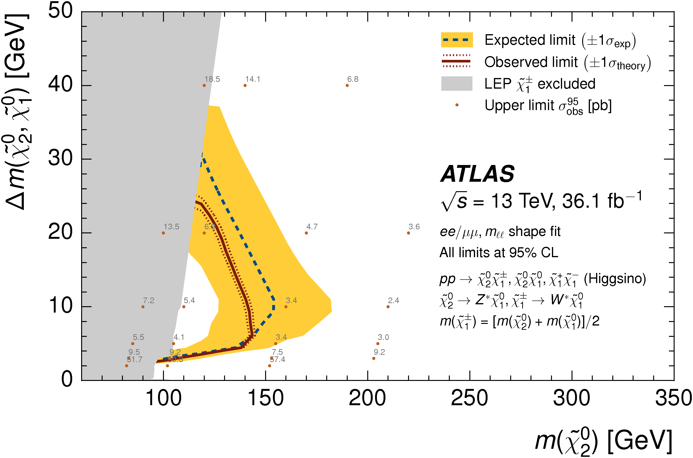
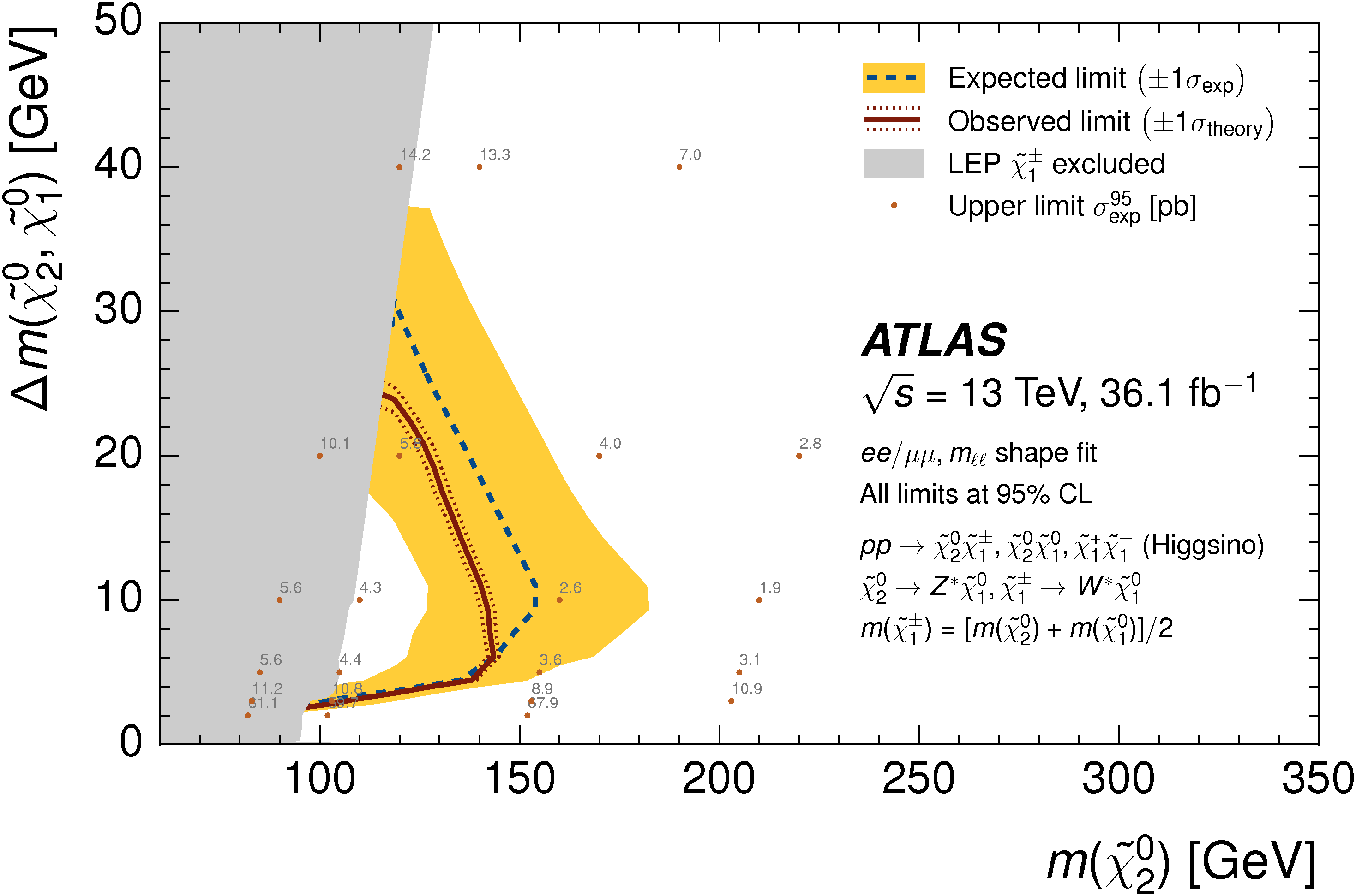
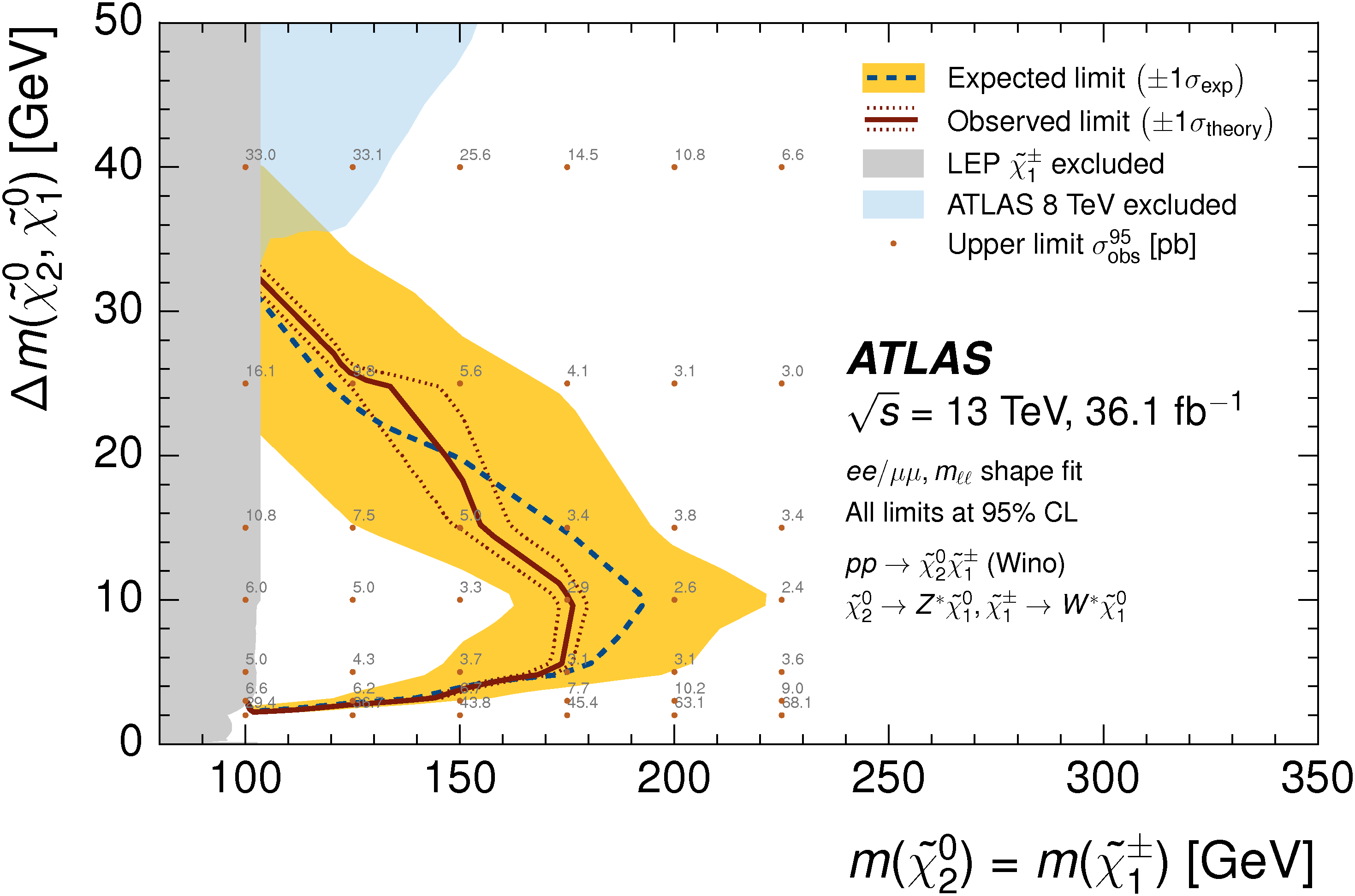
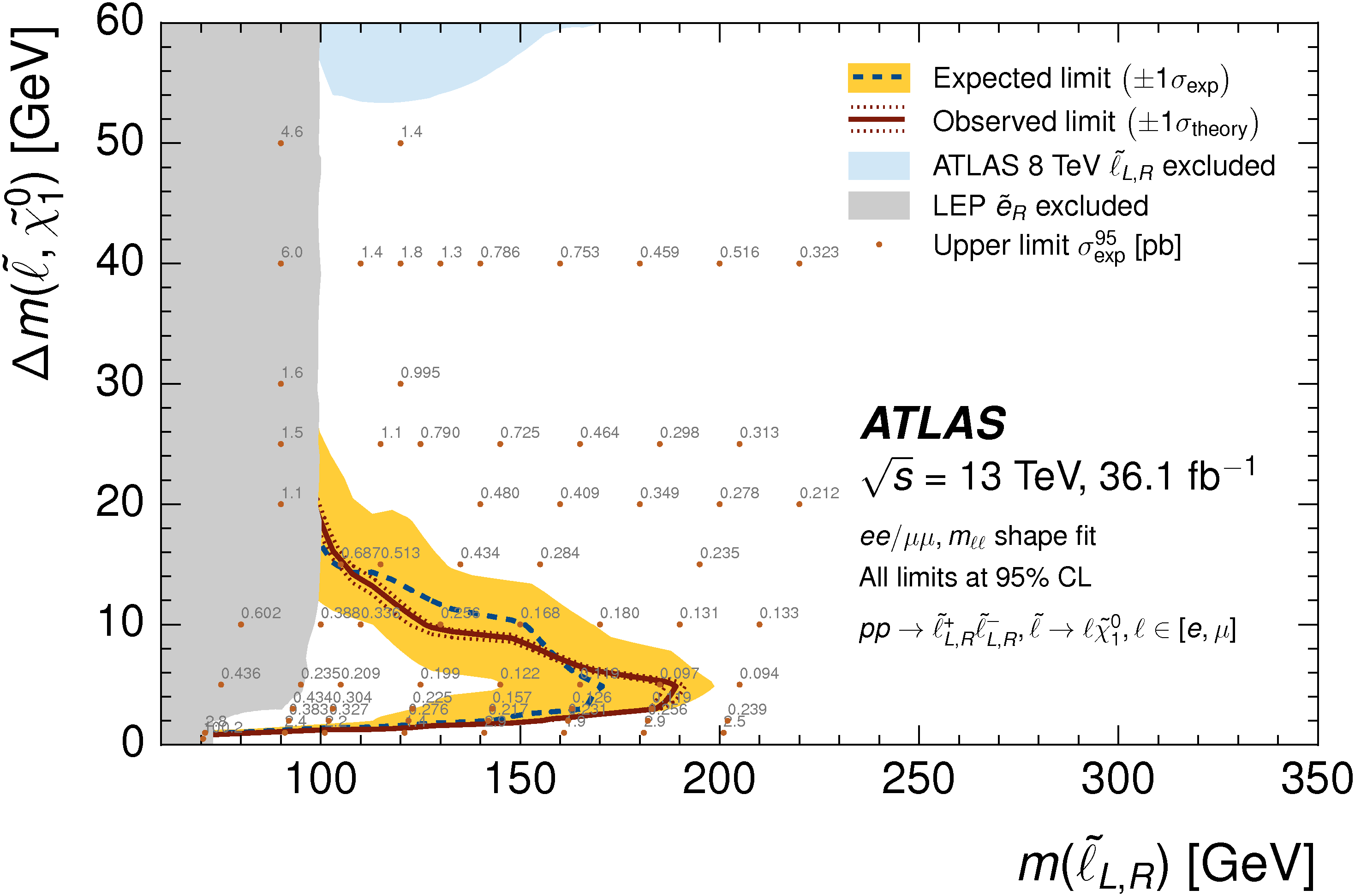
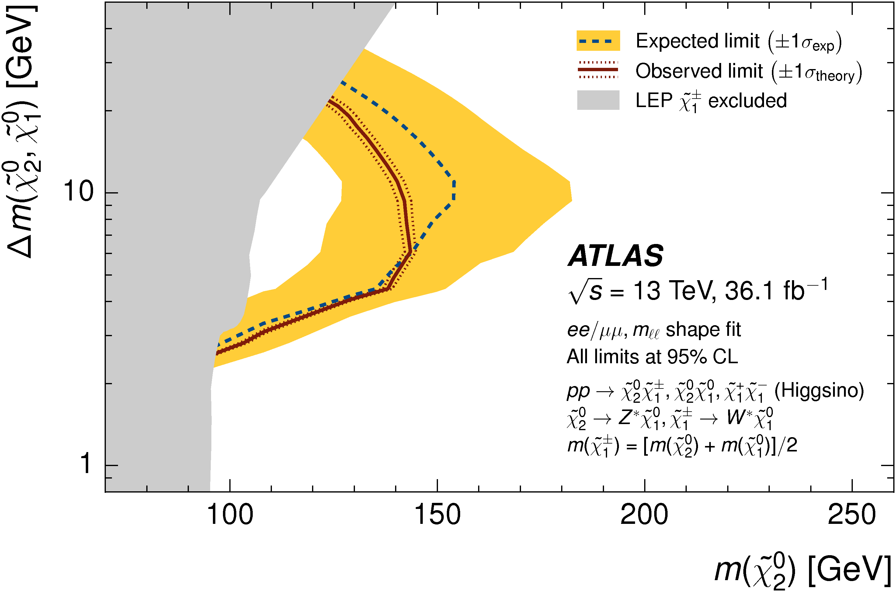
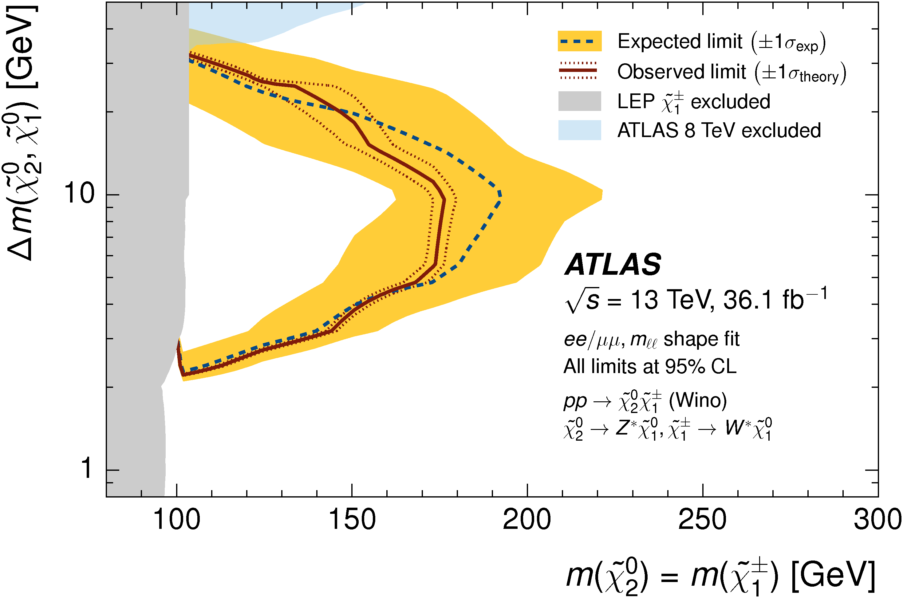
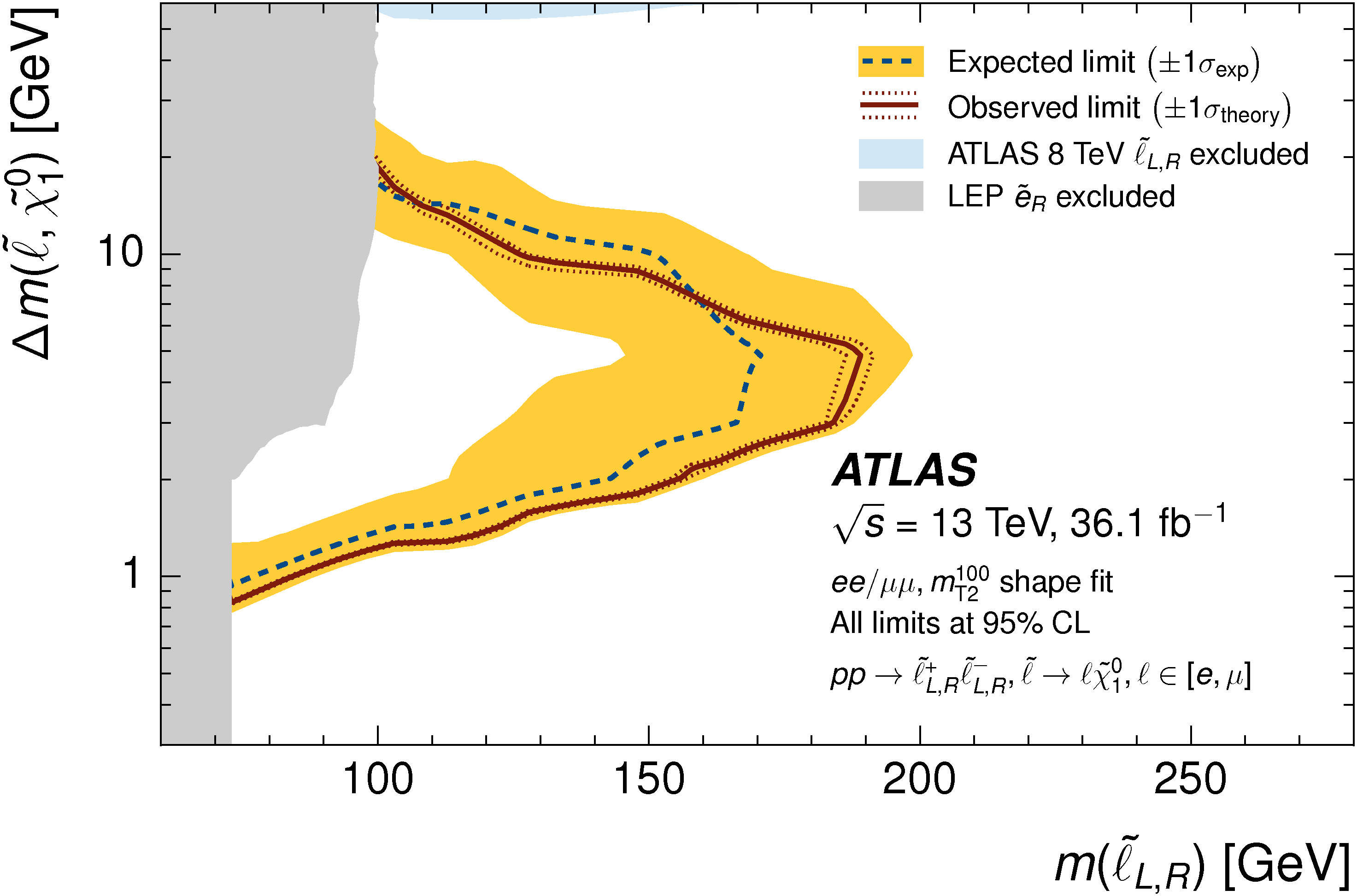
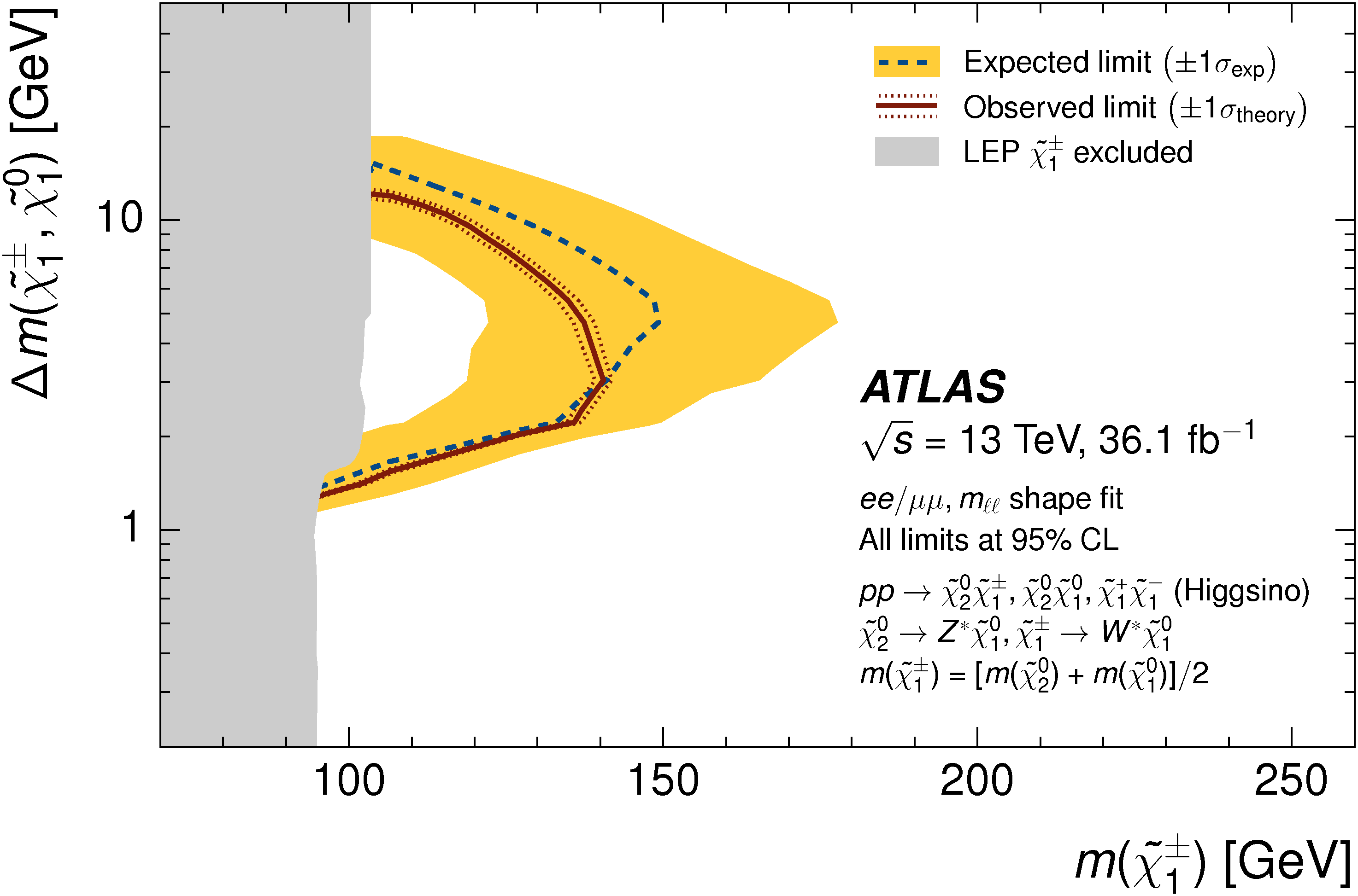
A search for electroweak production of supersymmetric particles in scenarios with compressed mass spectra in final states with two low-momentum leptons and missing transverse momentum is presented. This search uses proton-proton collision data recorded by the ATLAS detector at the Large Hadron Collider in 2015-2016, corresponding to 36.1 fb$^{-1}$ of integrated luminosity at $\sqrt{s}=13$ TeV. Events with same-flavor pairs of electrons or muons with opposite electric charge are selected. The data are found to be consistent with the Standard Model prediction. Results are interpreted using simplified models of R-parity-conserving supersymmetry in which there is a small mass difference between the masses of the produced supersymmetric particles and the lightest neutralino. Exclusion limits at 95% confidence level are set on next-to-lightest neutralino masses of up to 130 GeV for Higgsino production and 170 GeV for wino production, and sleptons masses of up to 180 GeV for pair production of sleptons. In the compressed mass regime, the exclusion limits extend down to mass splittings of 3 GeV for Higgsino production, 2.5 GeV for wino production, and 1 GeV for slepton production. The results are also interpreted in the context of a radiatively-driven natural supersymmetry model with non-universal Higgs boson masses.
Figures
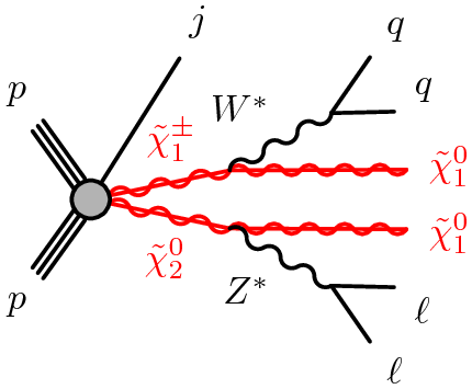
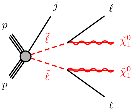
Figure 01a: Diagrams representing the two-lepton final state of (a) electroweakino χ̃₂⁰χ̃₁^± and (b) slepton pair ℓ̃ℓ̃ production in association with a jet radiated from the initial state (labeled j). The Higgsino simplified model also considers χ̃₂⁰χ̃₁⁰ and χ̃₁⁺χ̃₁^- production. png (18kB) pdf (35kB)
Figure 01b: Diagrams representing the two-lepton final state of (a) electroweakino χ̃₂⁰χ̃₁^± and (b) slepton pair ℓ̃ℓ̃ production in association with a jet radiated from the initial state (labeled j). The Higgsino simplified model also considers χ̃₂⁰χ̃₁⁰ and χ̃₁⁺χ̃₁^- production. png (15kB) pdf (26kB)
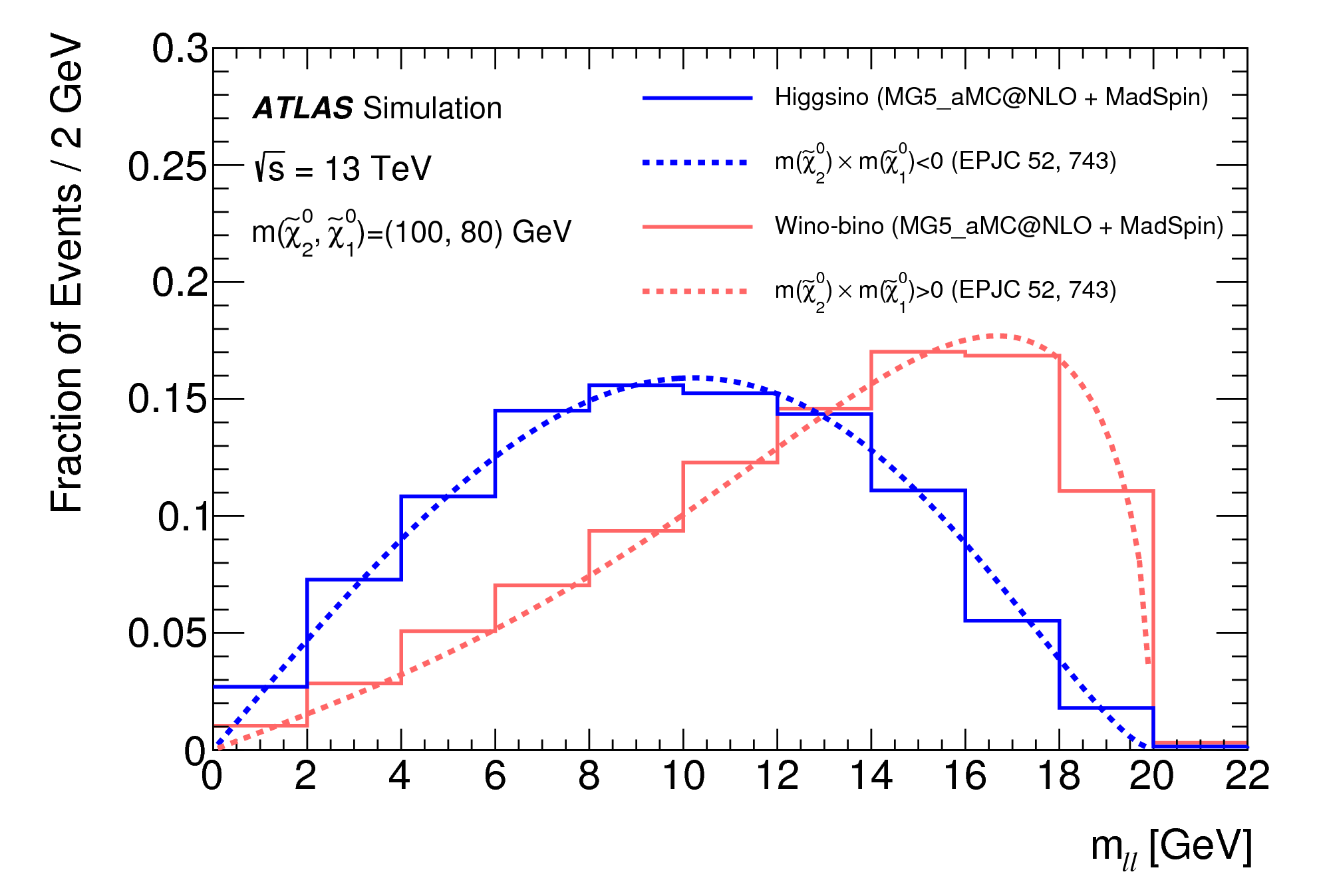
Figure 02: Dilepton invariant mass (m_ℓℓ) for Higgsino (H̃) and wino--bino (W̃/B̃) simplified models. The endpoint of the m_ℓℓ distribution is determined by the difference between the masses of the χ̃₂⁰ and χ̃₁⁰. The results from simulation (solid) are compared with an analytic calculation of the expected lineshape (dashed), where the product of the signed mass eigenvalues (m(χ̃₂⁰)× m(χ̃₁⁰)) is negative for Higgsino and positive for wino--bino scenarios. png (57kB) pdf (16kB)
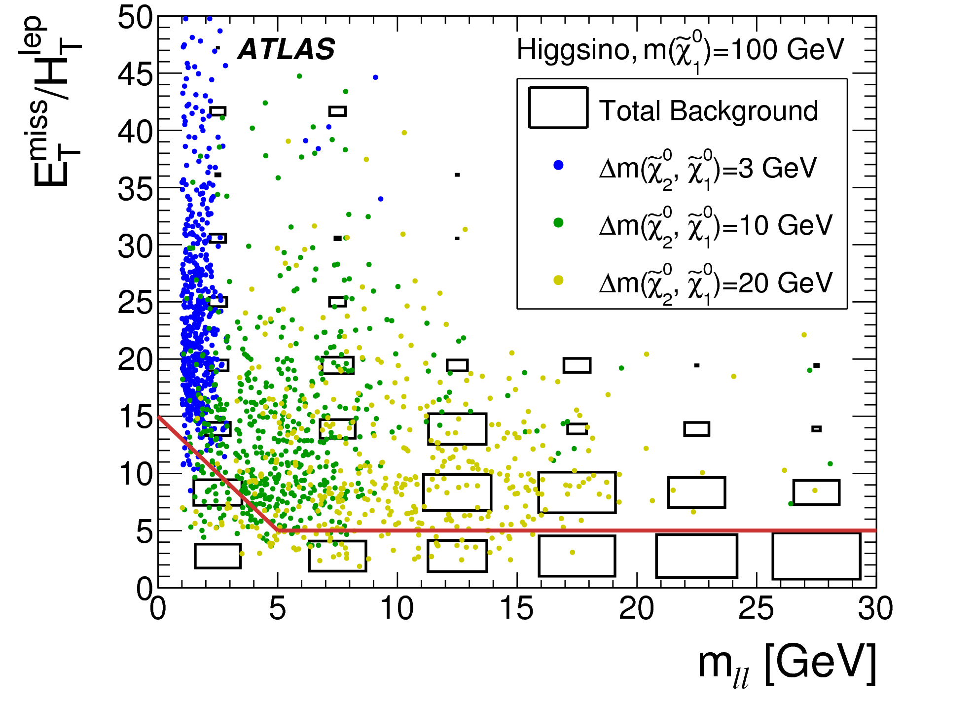
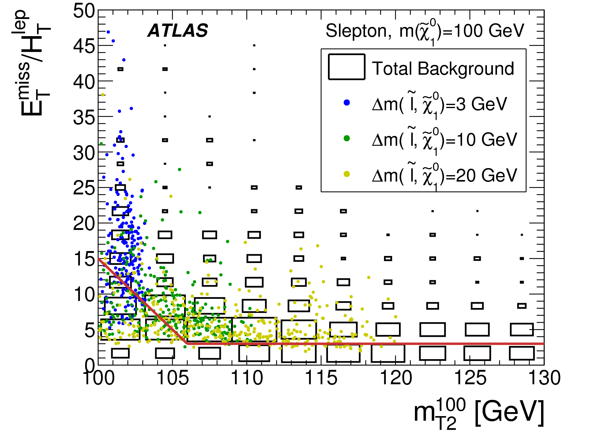
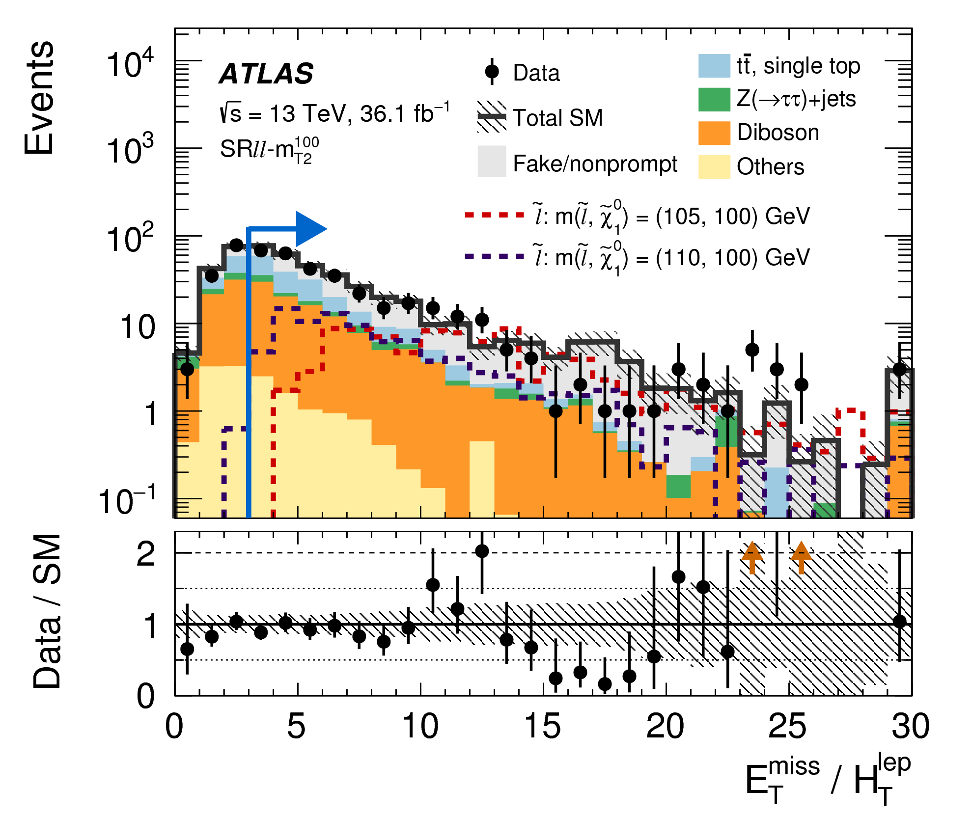
Figure 03a: Distributions of E_T^miss/H_T^lep for the electroweakino (left) and slepton (right) SRs, after applying all signal region selection criteria except those on E_T^miss/H_T^lep, m_ℓℓ, and m_T2. The solid red line indicates the requirement applied in the signal region; events in the region below the red line are rejected. Representative benchmark signals for the Higgsino (left) and slepton (right) simplified models are shown as circles. Both signal and background are normalized to their expected yields in 36.1 fb^-1. The total background includes the MC prediction for all the processes listed in Table 1 and a data-driven estimate for fake/nonprompt leptons discussed further in Section 6. png (210kB) pdf (55kB)
Figure 03b: Distributions of E_T^miss/H_T^lep for the electroweakino (left) and slepton (right) SRs, after applying all signal region selection criteria except those on E_T^miss/H_T^lep, m_ℓℓ, and m_T2. The solid red line indicates the requirement applied in the signal region; events in the region below the red line are rejected. Representative benchmark signals for the Higgsino (left) and slepton (right) simplified models are shown as circles. Both signal and background are normalized to their expected yields in 36.1 fb^-1. The total background includes the MC prediction for all the processes listed in Table 1 and a data-driven estimate for fake/nonprompt leptons discussed further in Section 6. png (160kB) pdf (39kB)
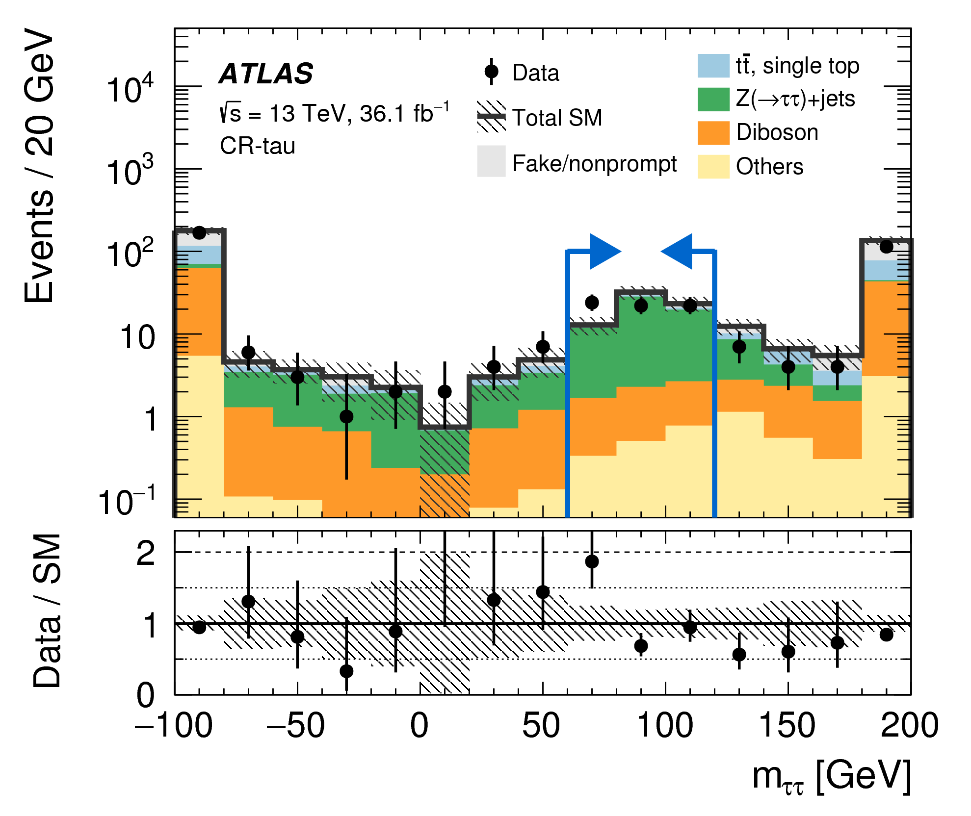
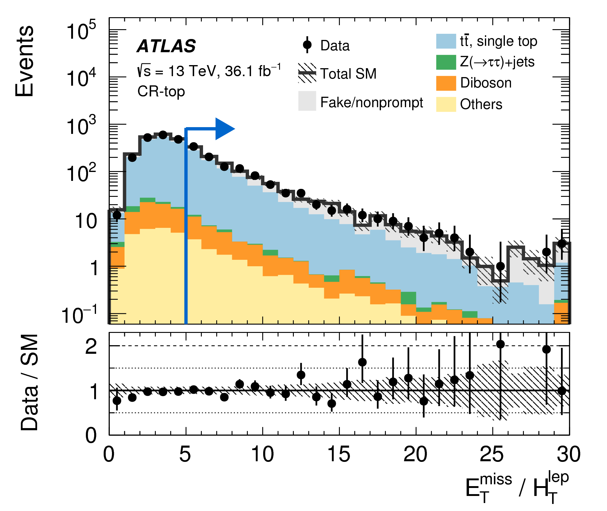
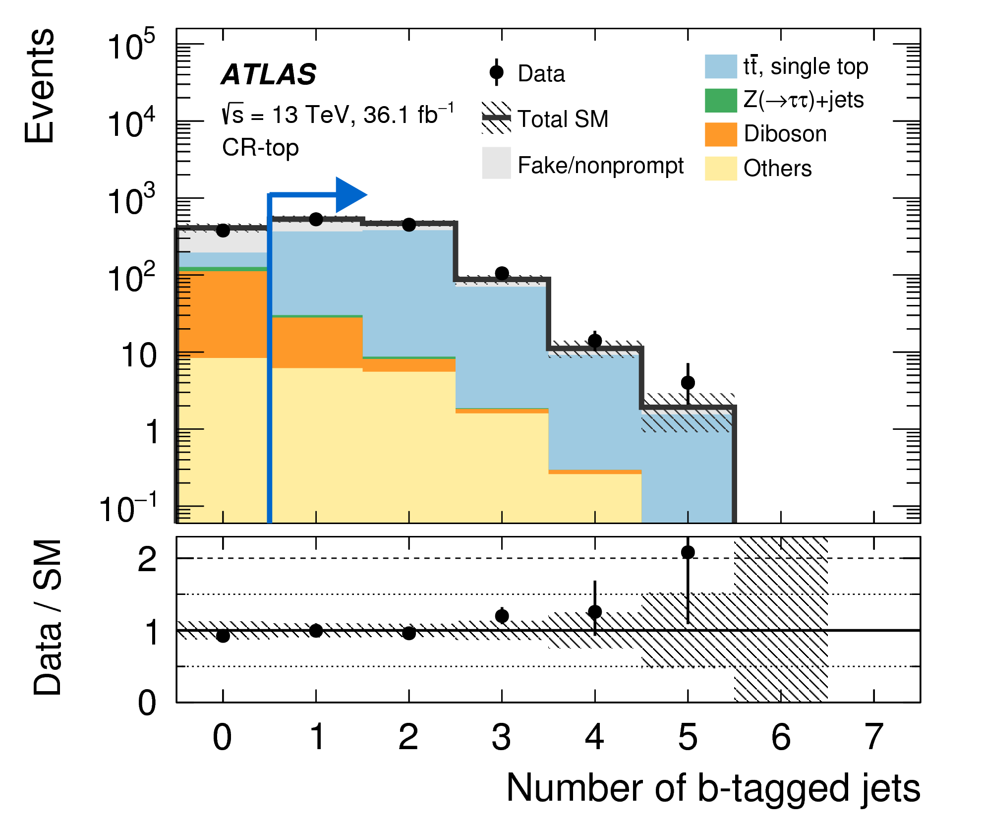
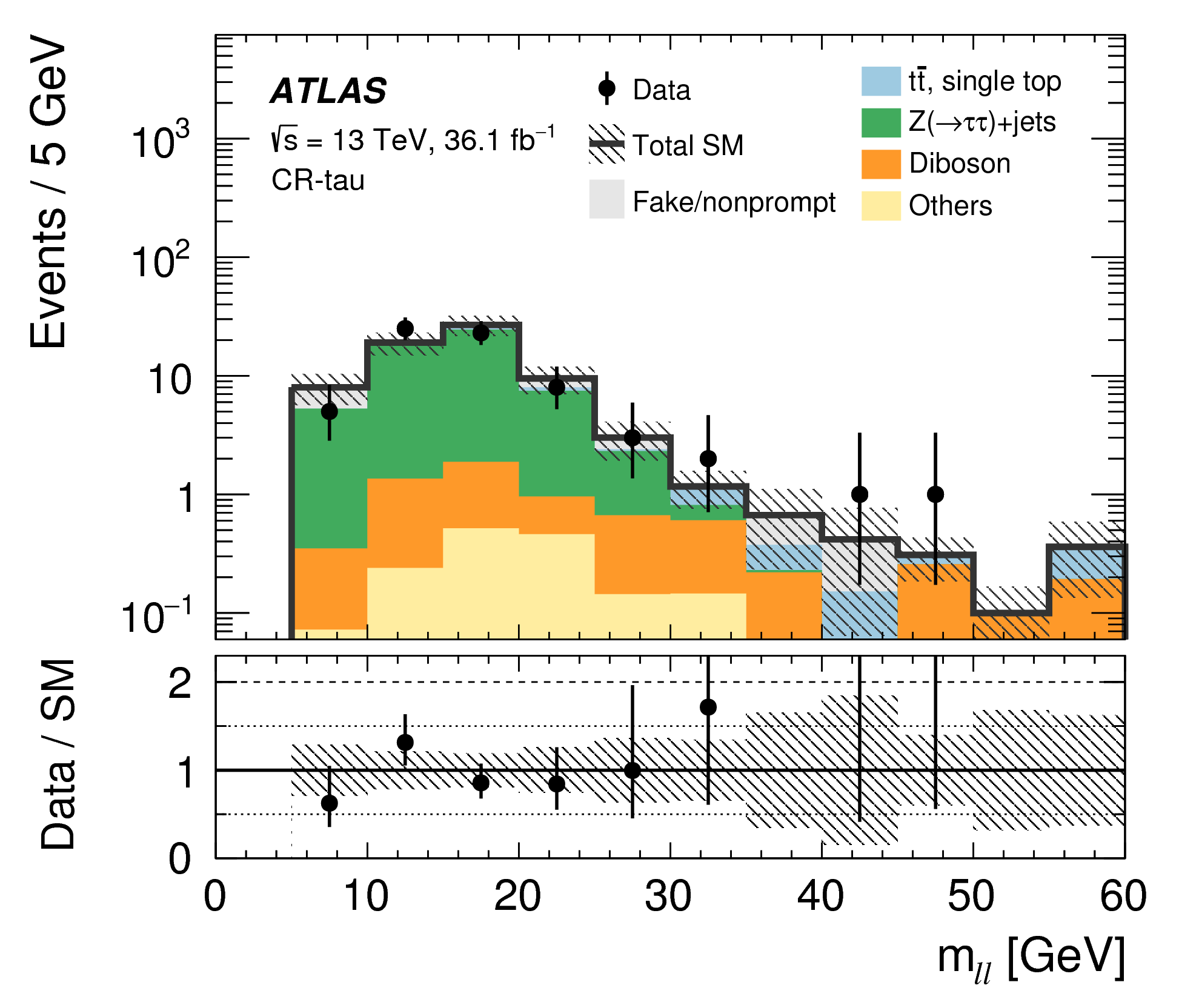
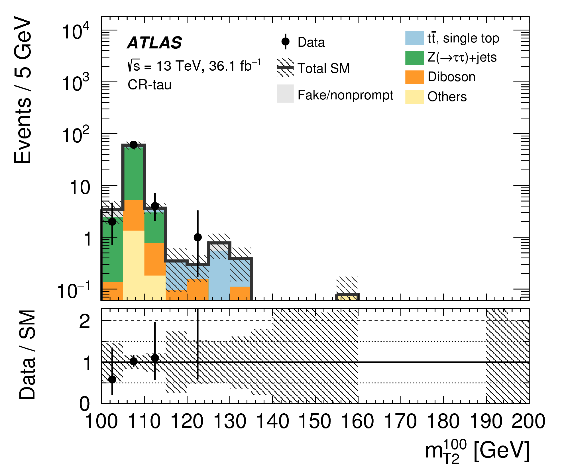
Figure 04a: Examples of kinematic distributions after the background-only fit showing the data as well as the expected background in control regions CR-tau (left) and CR-top (right). The full event selection of the corresponding regions is applied, except for the requirement that is imposed on the variable being plotted. This requirement is indicated by blue arrows in the distributions. The first (last) bin includes underflow (overflow). Background processes containing fewer than two prompt leptons are categorized as `Fake/nonprompt'. The category `Others' contains rare backgrounds from triboson, Higgs boson, and the remaining top-quark production processes listed in Table 1. The uncertainty bands plotted include all statistical and systematic uncertainties. png (100kB) pdf (19kB)
Figure 04b: Examples of kinematic distributions after the background-only fit showing the data as well as the expected background in control regions CR-tau (left) and CR-top (right). The full event selection of the corresponding regions is applied, except for the requirement that is imposed on the variable being plotted. This requirement is indicated by blue arrows in the distributions. The first (last) bin includes underflow (overflow). Background processes containing fewer than two prompt leptons are categorized as `Fake/nonprompt'. The category `Others' contains rare backgrounds from triboson, Higgs boson, and the remaining top-quark production processes listed in Table 1. The uncertainty bands plotted include all statistical and systematic uncertainties. png (107kB) pdf (21kB)
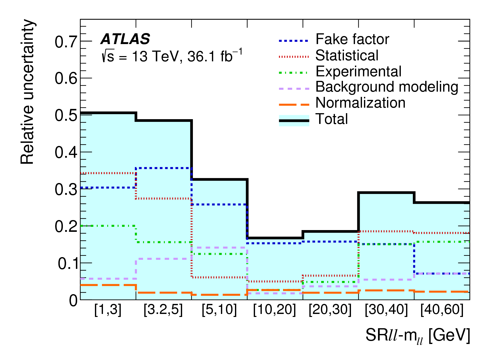
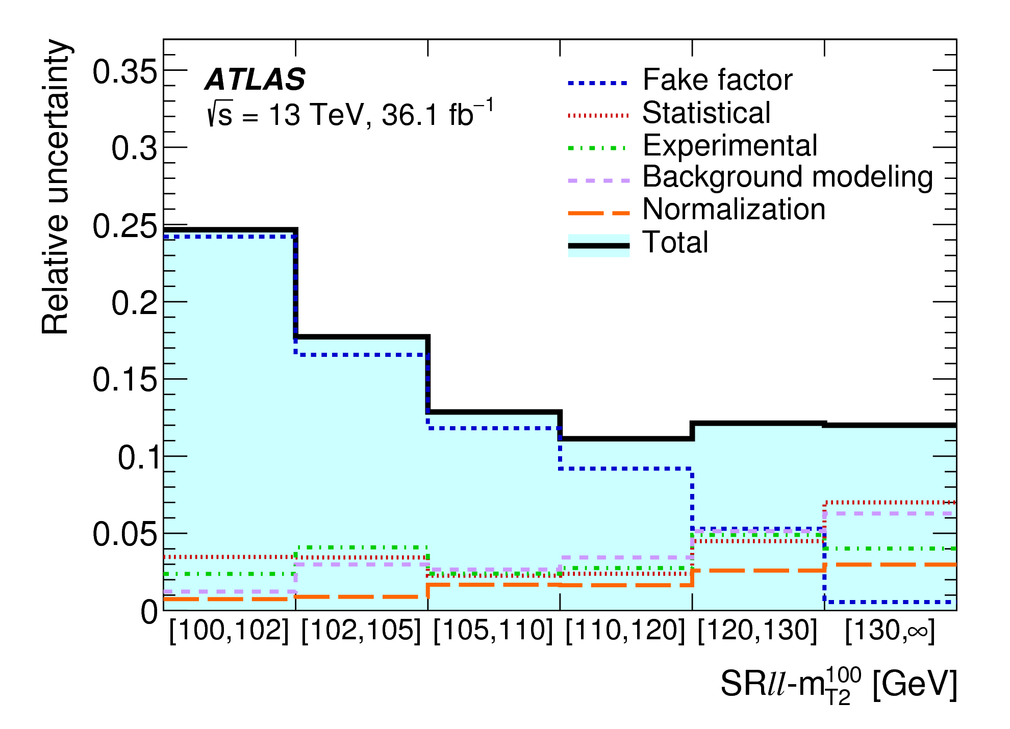
Figure 05a: The relative systematic uncertainties in the background prediction in the exclusive electroweakino (left) and slepton (right) SRs. The individual uncertainties can be correlated and do not necessarily add up in quadrature to the total uncertainty. png (64kB) pdf (14kB)
Figure 05b: The relative systematic uncertainties in the background prediction in the exclusive electroweakino (left) and slepton (right) SRs. The individual uncertainties can be correlated and do not necessarily add up in quadrature to the total uncertainty. png (39kB) pdf (14kB)
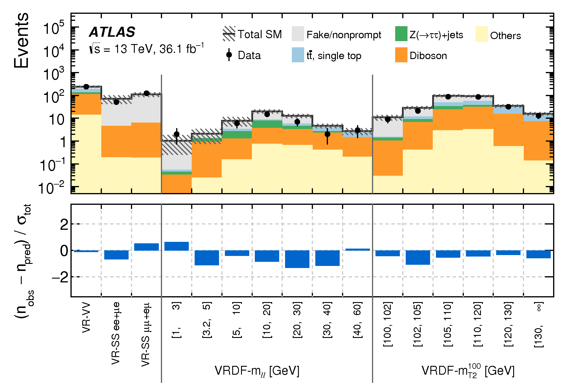
Figure 06: Comparison of observed and expected event yields in the validation regions after the background-only fit. Background processes containing fewer than two prompt leptons are categorized as `Fake/nonprompt'. The category `Others' contains rare backgrounds from triboson, Higgs boson, and the remaining top-quark production processes listed in Table 1. Uncertainties in the background estimates include both the statistical and systematic uncertainties, where σ_tot denotes the total uncertainty. png (27kB) pdf (20kB)
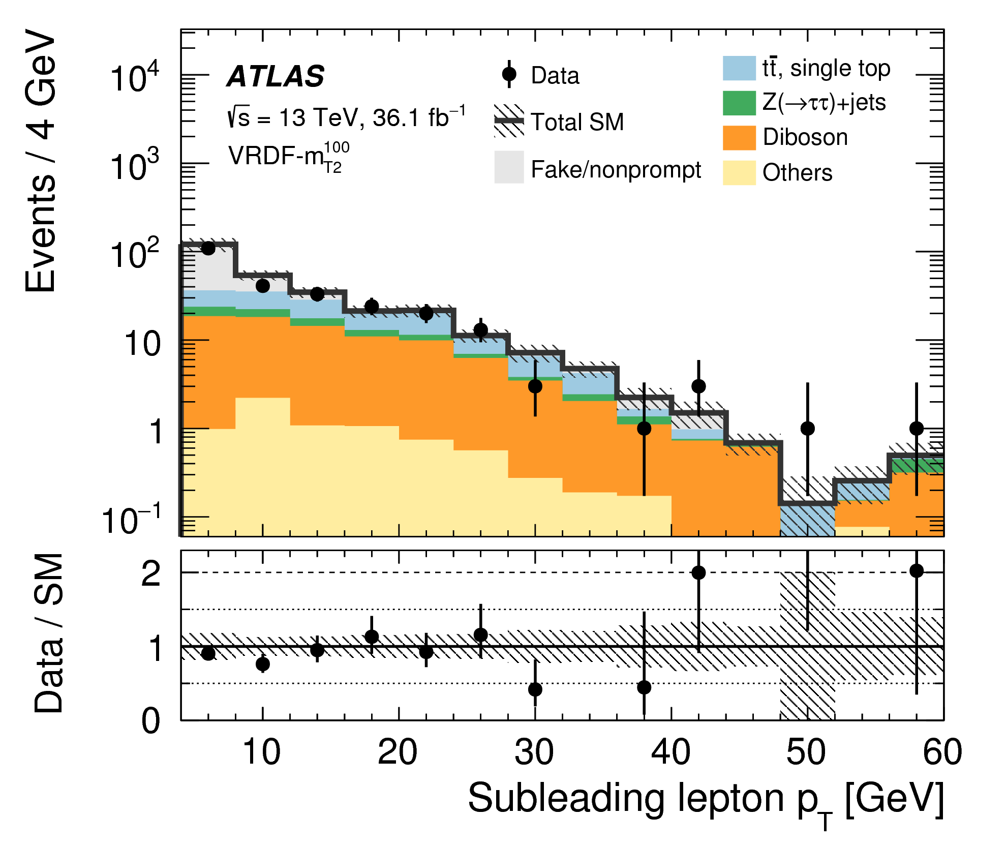
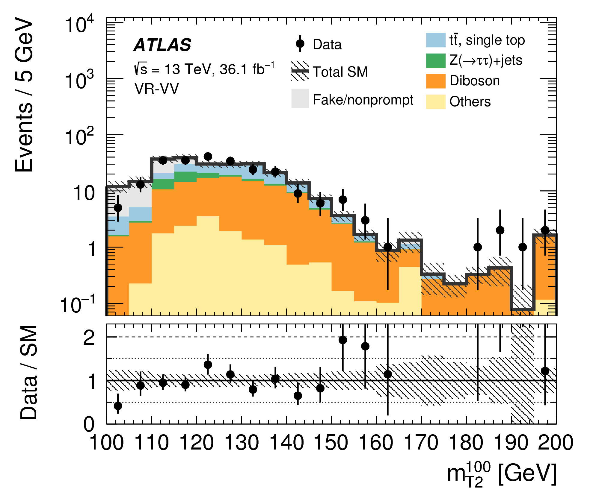
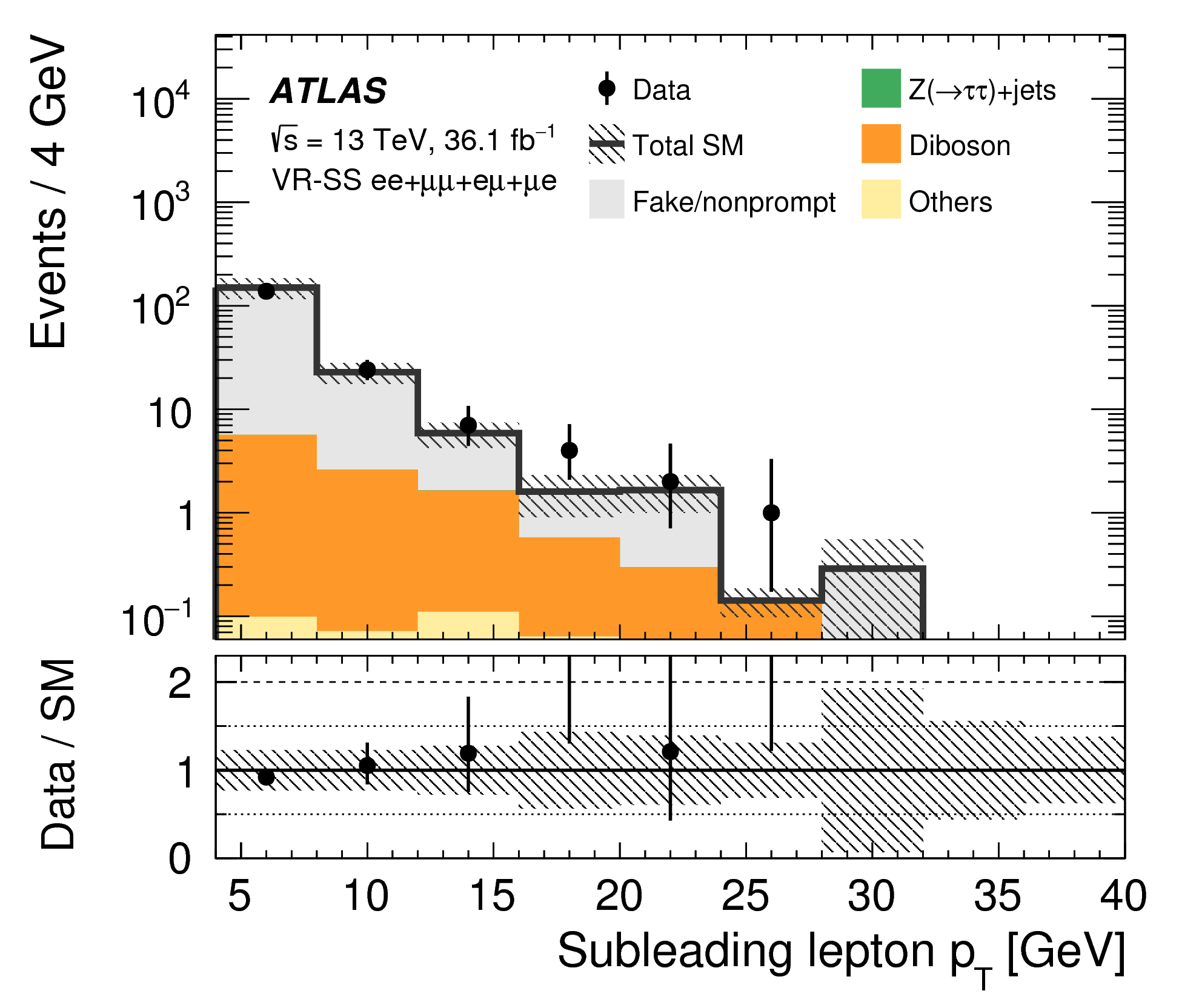
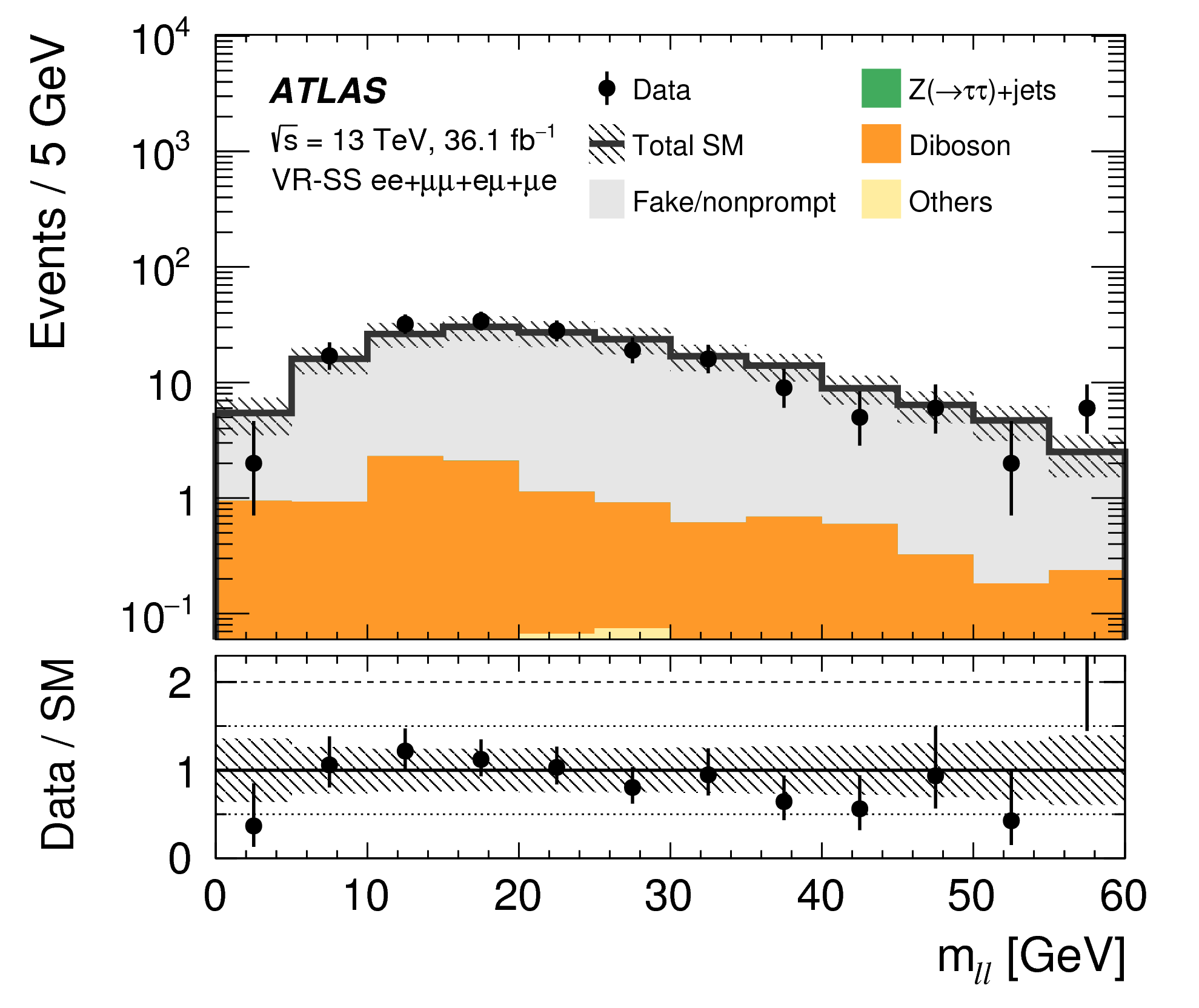
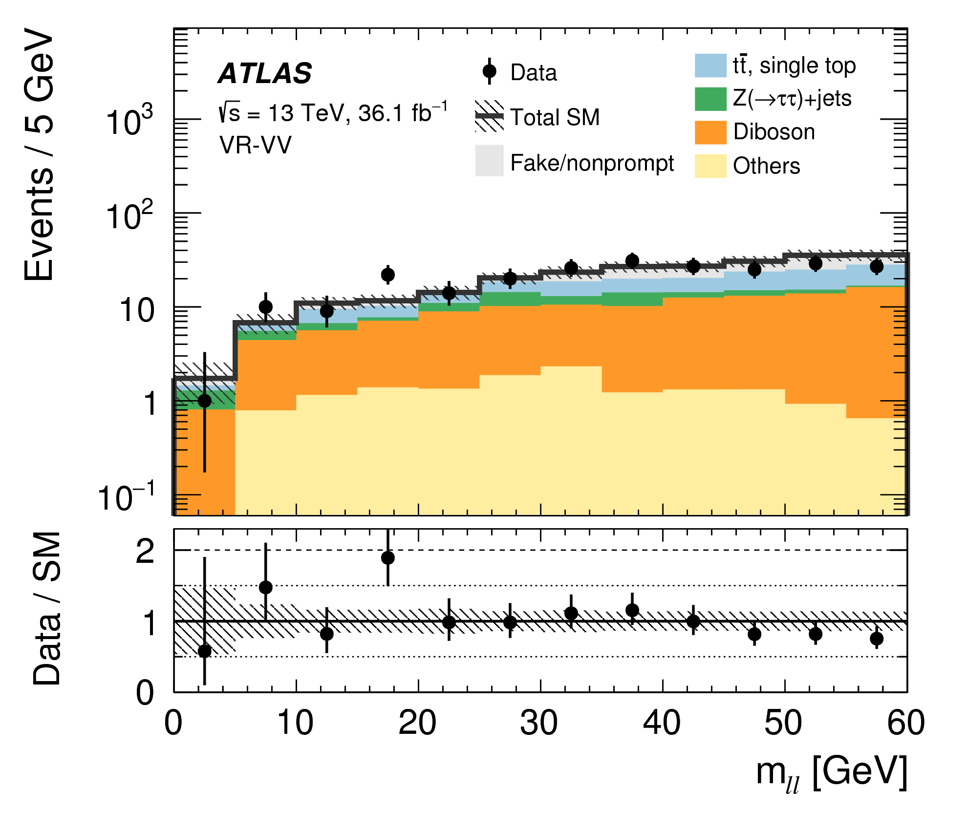
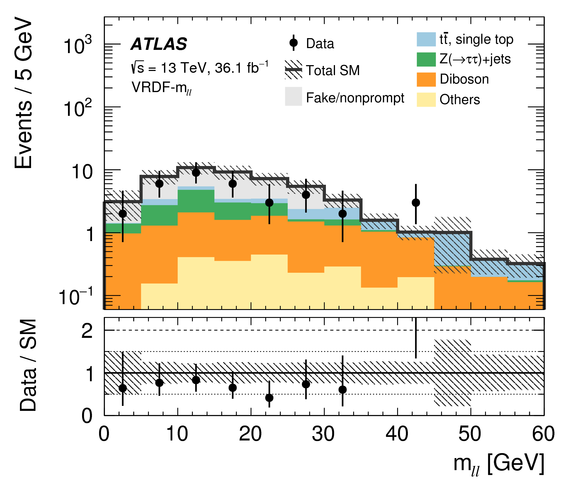
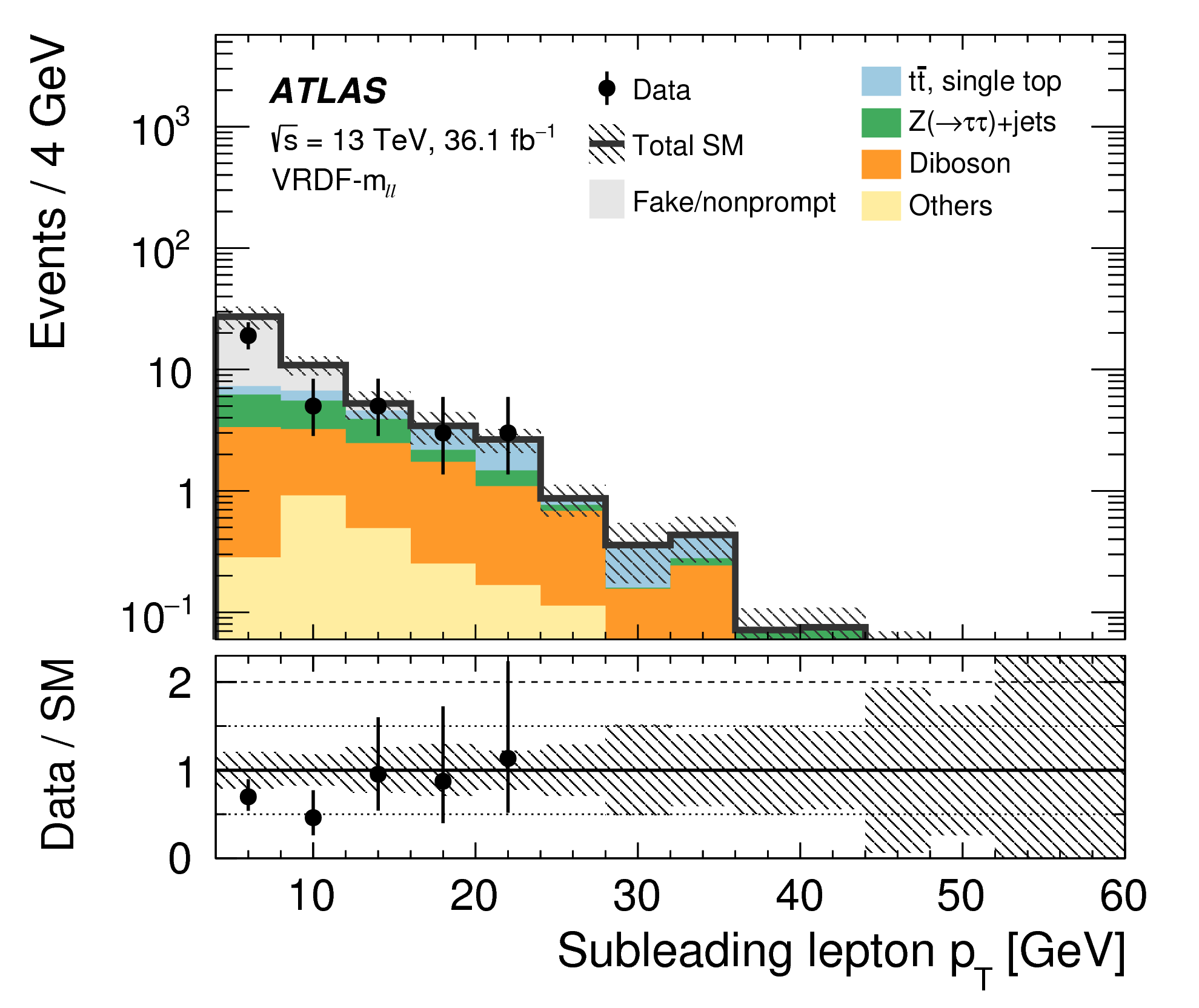
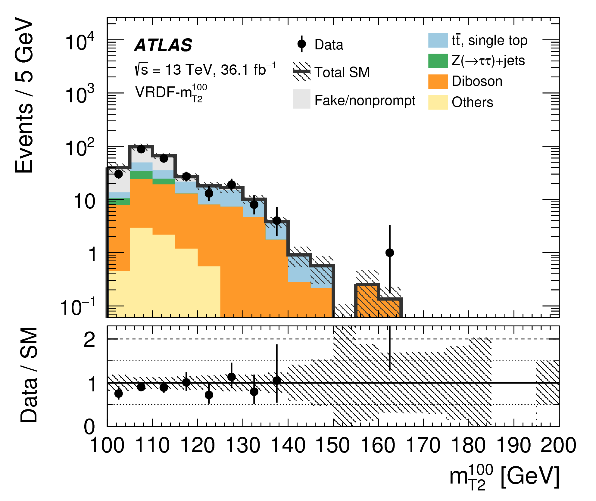
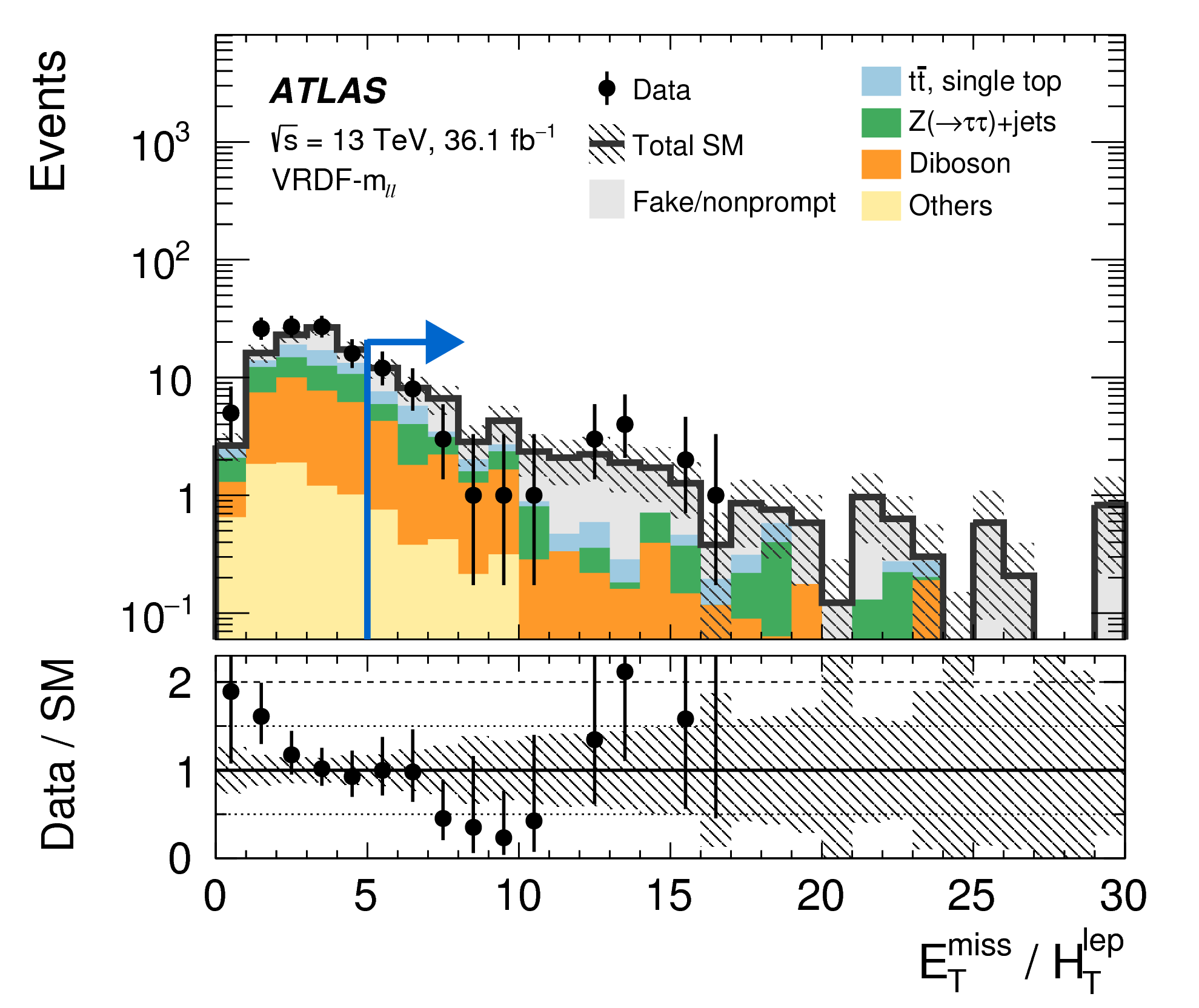
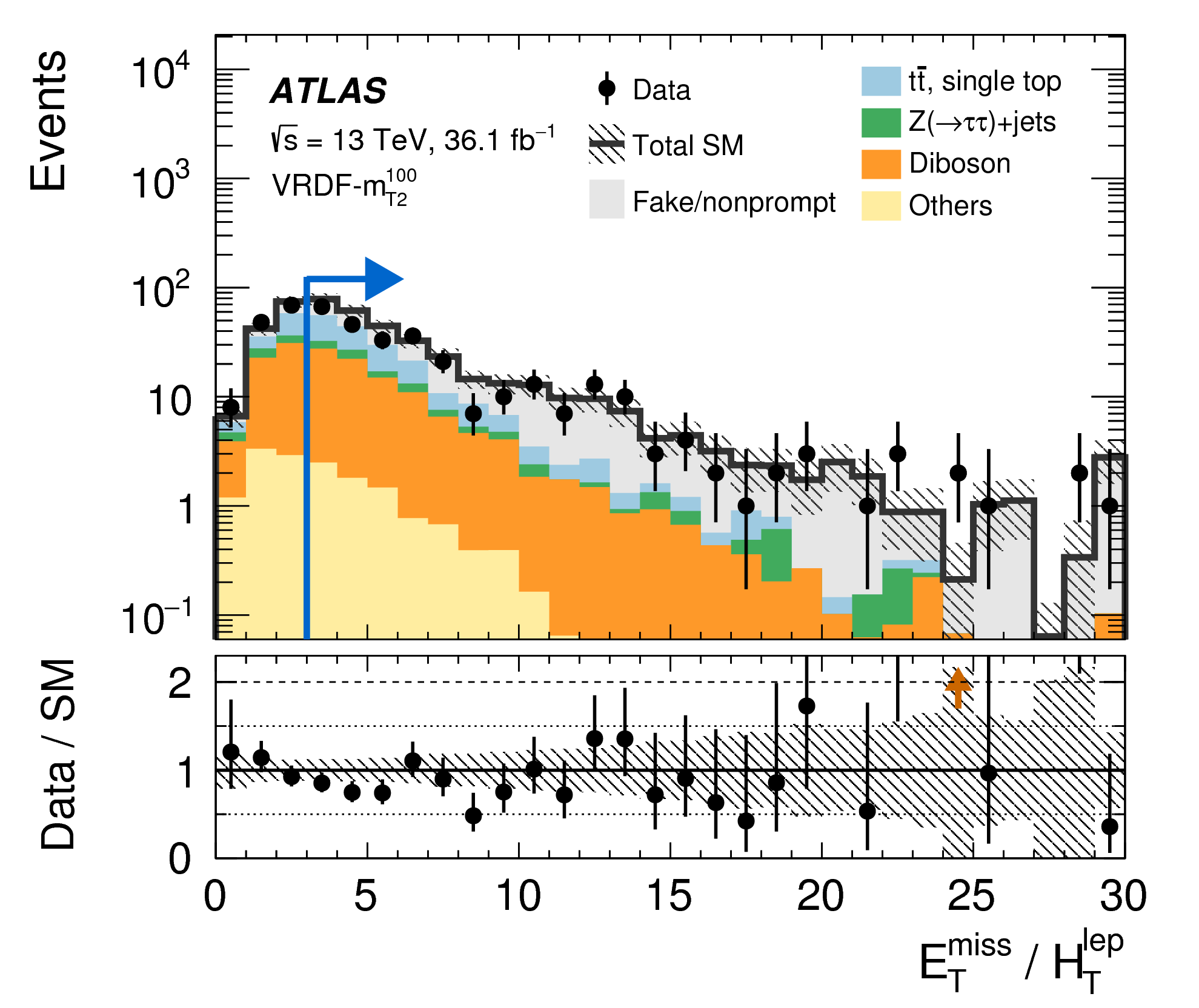
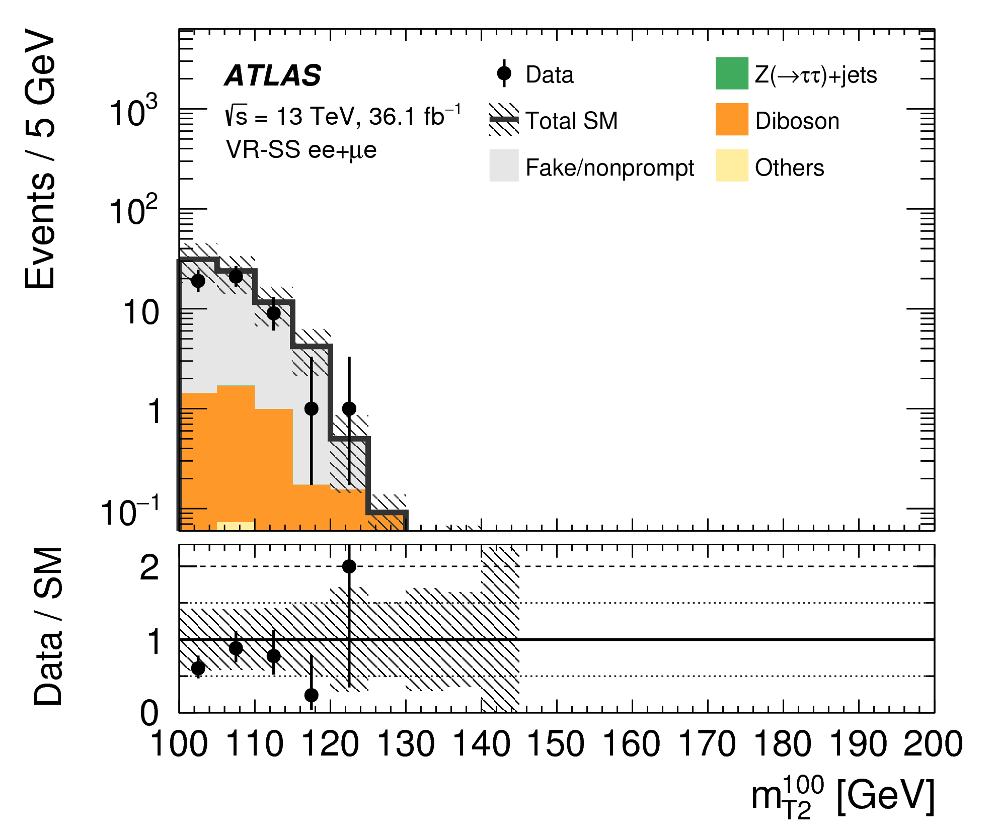
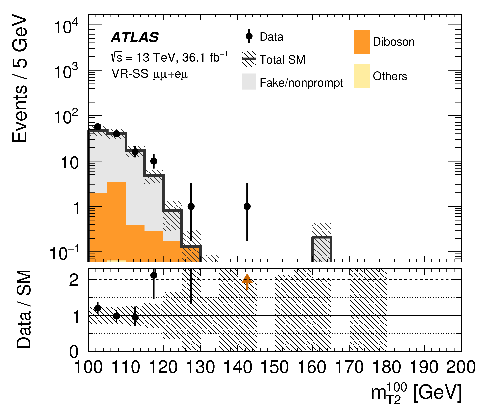
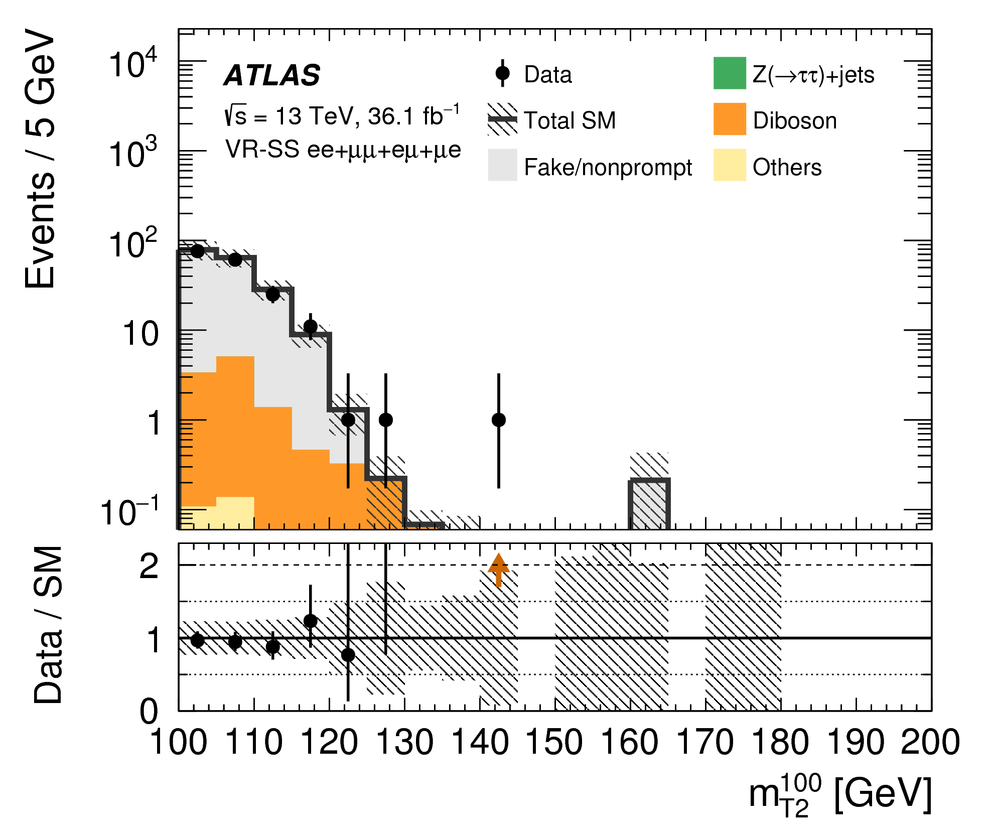
Figure 07a: Kinematic distributions after the background-only fit showing the data and the expected background in the different-flavor validation region VRDF-m_T2¹⁰⁰ (top left), the diboson validation region VR-VV (top right), and the same-sign validation region VR-SS inclusive of lepton flavor (bottom). Similar levels of agreement are observed in other kinematic distributions for VR-SS and VR-VV. Background processes containing fewer than two prompt leptons are categorized as `Fake/nonprompt'. The category `Others' contains rare backgrounds from triboson, Higgs boson, and the remaining top-quark production processes listed in Table 1. The last bin includes overflow. The uncertainty bands plotted include all statistical and systematic uncertainties. Orange arrows in the Data/SM panel indicate values that are beyond the y-axis range. png (92kB) pdf (18kB)
Figure 07b: Kinematic distributions after the background-only fit showing the data and the expected background in the different-flavor validation region VRDF-m_T2¹⁰⁰ (top left), the diboson validation region VR-VV (top right), and the same-sign validation region VR-SS inclusive of lepton flavor (bottom). Similar levels of agreement are observed in other kinematic distributions for VR-SS and VR-VV. Background processes containing fewer than two prompt leptons are categorized as `Fake/nonprompt'. The category `Others' contains rare backgrounds from triboson, Higgs boson, and the remaining top-quark production processes listed in Table 1. The last bin includes overflow. The uncertainty bands plotted include all statistical and systematic uncertainties. Orange arrows in the Data/SM panel indicate values that are beyond the y-axis range. png (98kB) pdf (20kB)
Figure 07c: Kinematic distributions after the background-only fit showing the data and the expected background in the different-flavor validation region VRDF-m_T2¹⁰⁰ (top left), the diboson validation region VR-VV (top right), and the same-sign validation region VR-SS inclusive of lepton flavor (bottom). Similar levels of agreement are observed in other kinematic distributions for VR-SS and VR-VV. Background processes containing fewer than two prompt leptons are categorized as `Fake/nonprompt'. The category `Others' contains rare backgrounds from triboson, Higgs boson, and the remaining top-quark production processes listed in Table 1. The last bin includes overflow. The uncertainty bands plotted include all statistical and systematic uncertainties. Orange arrows in the Data/SM panel indicate values that are beyond the y-axis range. png (49kB) pdf (17kB)
Figure 07d: Kinematic distributions after the background-only fit showing the data and the expected background in the different-flavor validation region VRDF-m_T2¹⁰⁰ (top left), the diboson validation region VR-VV (top right), and the same-sign validation region VR-SS inclusive of lepton flavor (bottom). Similar levels of agreement are observed in other kinematic distributions for VR-SS and VR-VV. Background processes containing fewer than two prompt leptons are categorized as `Fake/nonprompt'. The category `Others' contains rare backgrounds from triboson, Higgs boson, and the remaining top-quark production processes listed in Table 1. The last bin includes overflow. The uncertainty bands plotted include all statistical and systematic uncertainties. Orange arrows in the Data/SM panel indicate values that are beyond the y-axis range. png (47kB) pdf (18kB)
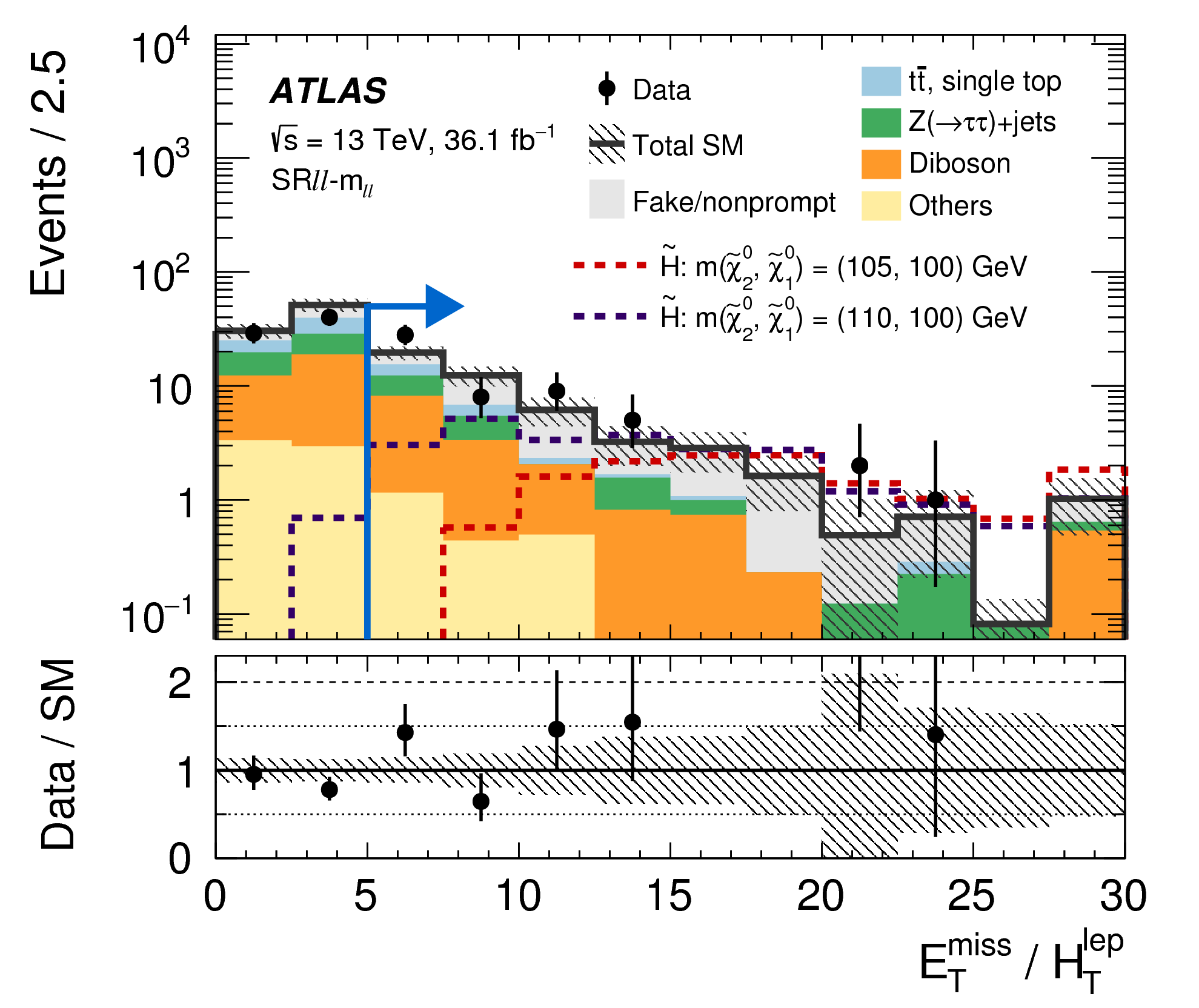
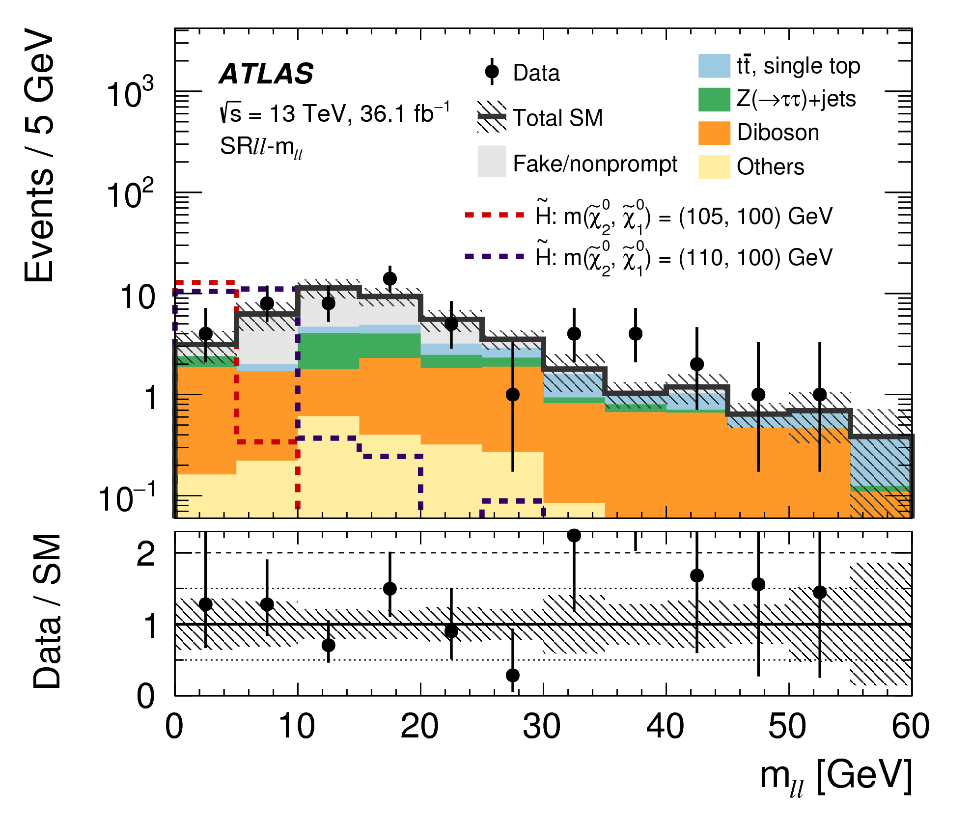
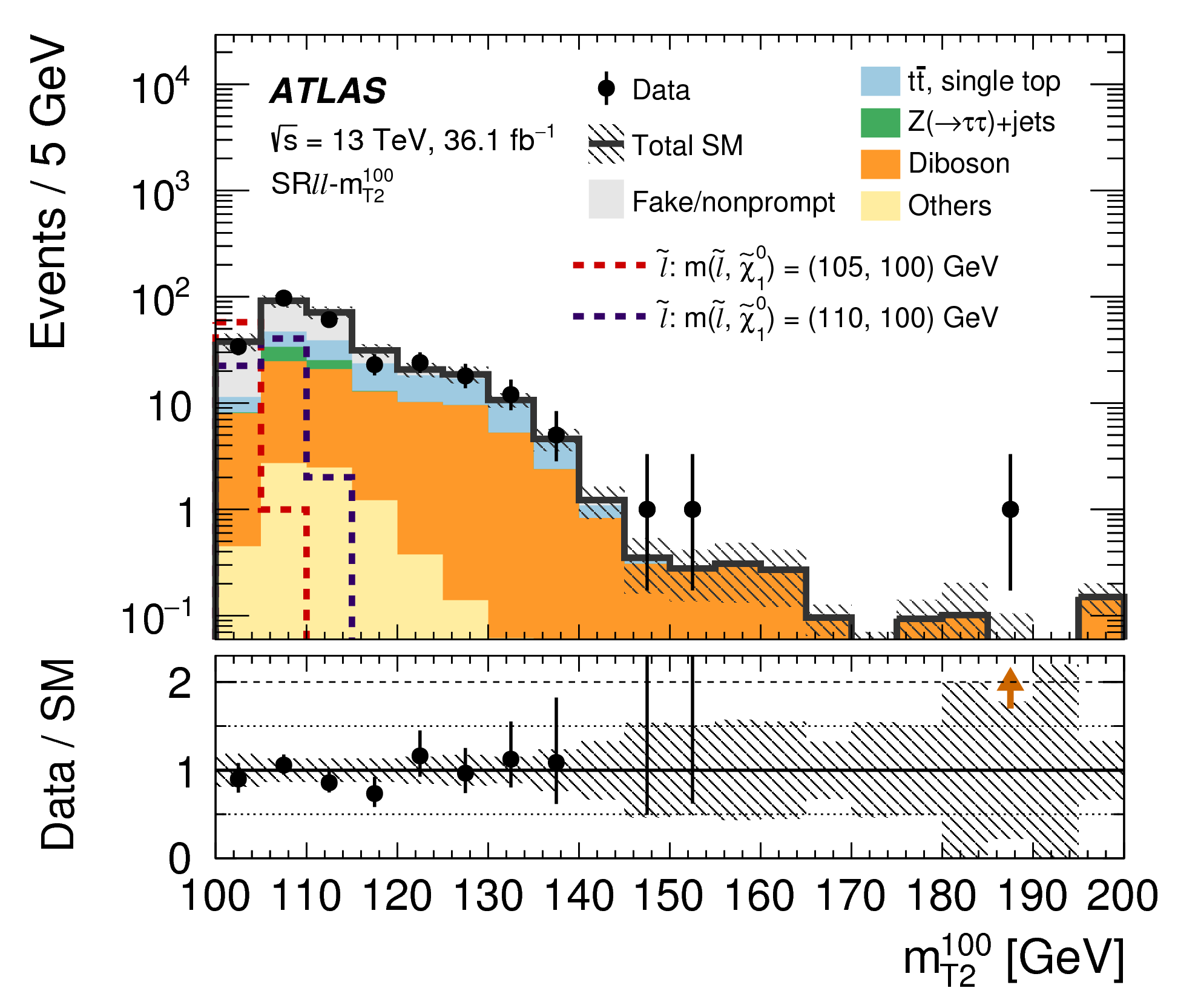
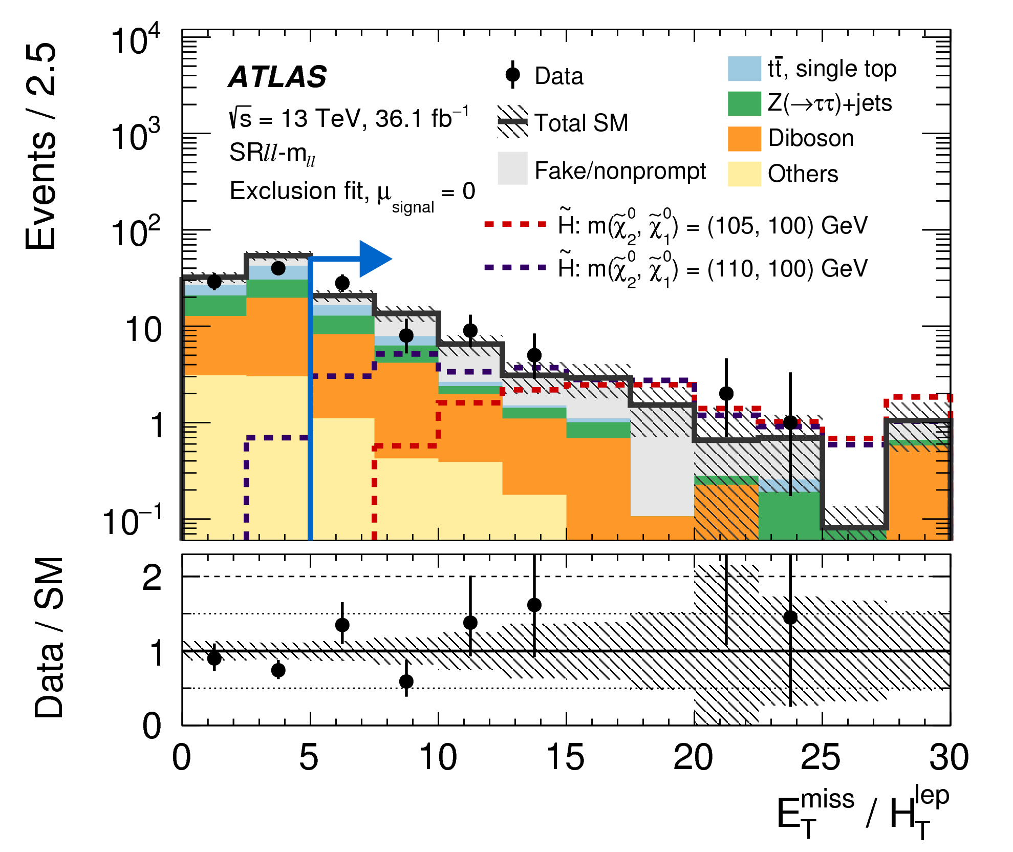
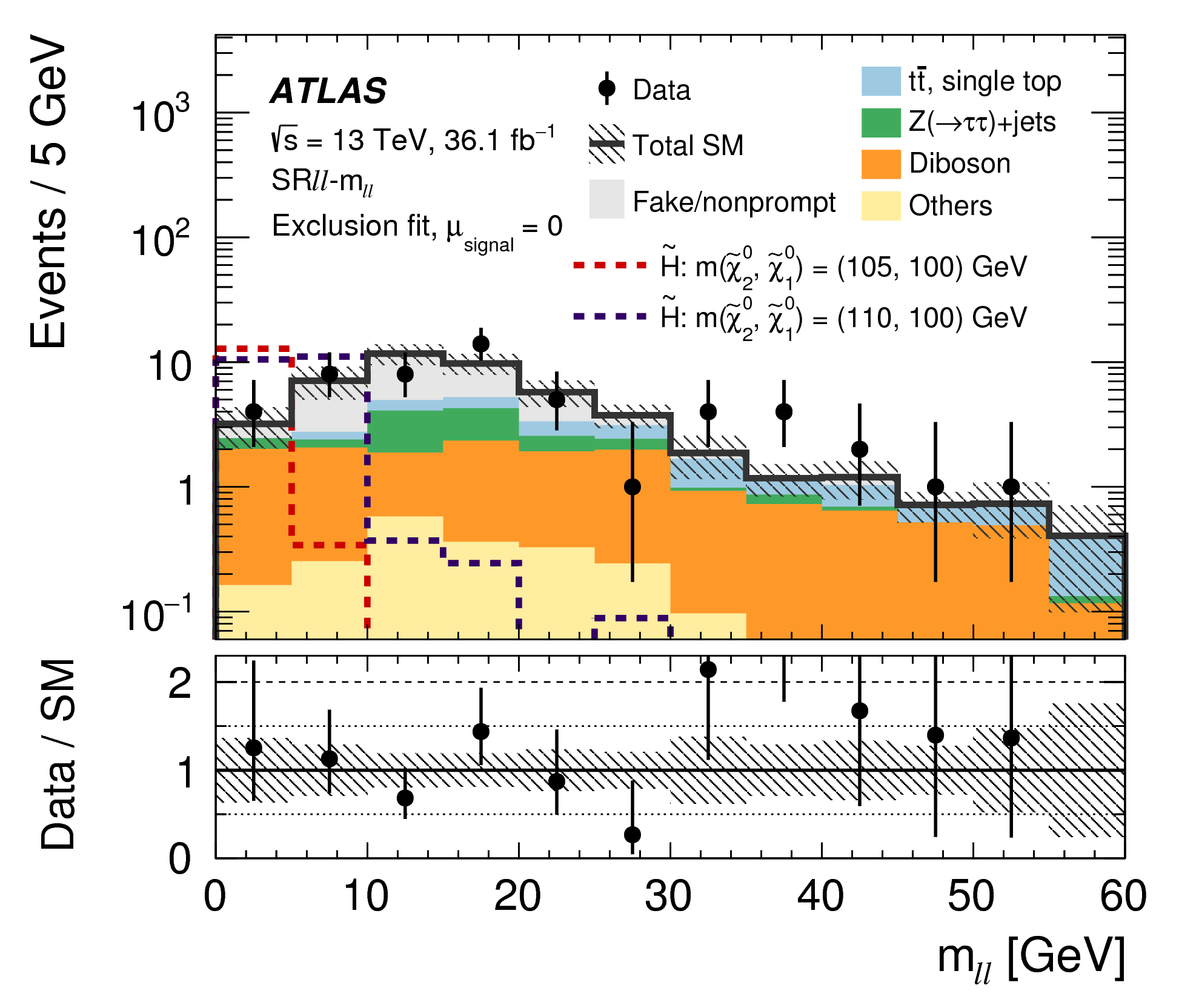
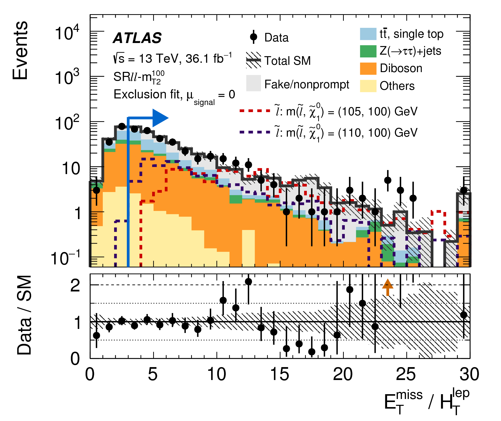
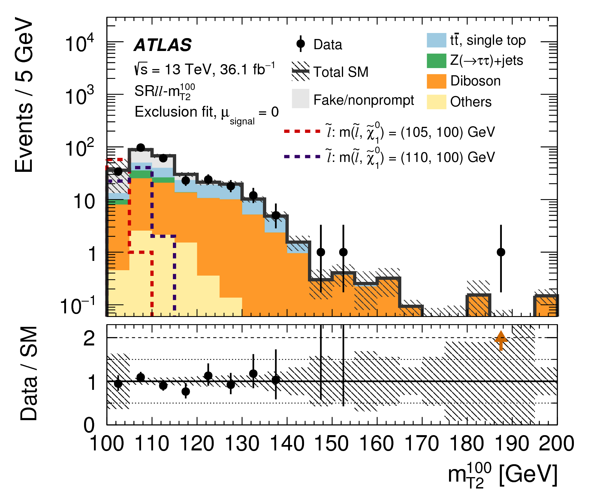
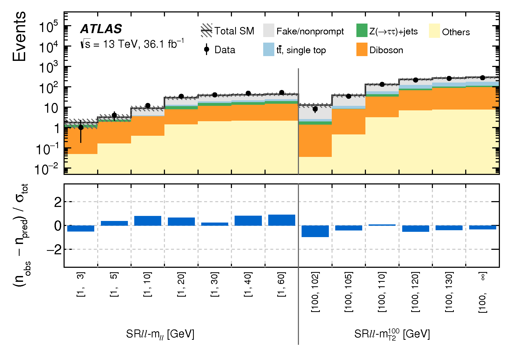
Figure 08a: Kinematic distributions after the background-only fit showing the data as well as the expected background in the inclusive electroweakino SRℓℓ-m_ℓℓ [1, 60] (top) and slepton SRℓℓ-m_T2¹⁰⁰ [100, ∞] (bottom) signal regions. The arrow in the E_T^miss/H_T^lep variables indicates the minimum value of the requirement imposed in the final SR selection. The m_ℓℓ and m_T2 distributions (right) have all the SR requirements applied. Background processes containing fewer than two prompt leptons are categorized as `Fake/nonprompt'. The category `Others' contains rare backgrounds from triboson, Higgs boson, and the remaining top-quark production processes listed in Table 1. The uncertainty bands plotted include all statistical and systematic uncertainties. The last bin includes overflow. The dashed lines represent benchmark signal samples corresponding to the Higgsino H̃ and slepton ℓ̃ simplified models. Orange arrows in the Data/SM panel indicate values that are beyond the y-axis range. png (109kB) pdf (18kB)
Figure 08b: Kinematic distributions after the background-only fit showing the data as well as the expected background in the inclusive electroweakino SRℓℓ-m_ℓℓ [1, 60] (top) and slepton SRℓℓ-m_T2¹⁰⁰ [100, ∞] (bottom) signal regions. The arrow in the E_T^miss/H_T^lep variables indicates the minimum value of the requirement imposed in the final SR selection. The m_ℓℓ and m_T2 distributions (right) have all the SR requirements applied. Background processes containing fewer than two prompt leptons are categorized as `Fake/nonprompt'. The category `Others' contains rare backgrounds from triboson, Higgs boson, and the remaining top-quark production processes listed in Table 1. The uncertainty bands plotted include all statistical and systematic uncertainties. The last bin includes overflow. The dashed lines represent benchmark signal samples corresponding to the Higgsino H̃ and slepton ℓ̃ simplified models. Orange arrows in the Data/SM panel indicate values that are beyond the y-axis range. png (109kB) pdf (18kB)
Figure 08c: Kinematic distributions after the background-only fit showing the data as well as the expected background in the inclusive electroweakino SRℓℓ-m_ℓℓ [1, 60] (top) and slepton SRℓℓ-m_T2¹⁰⁰ [100, ∞] (bottom) signal regions. The arrow in the E_T^miss/H_T^lep variables indicates the minimum value of the requirement imposed in the final SR selection. The m_ℓℓ and m_T2 distributions (right) have all the SR requirements applied. Background processes containing fewer than two prompt leptons are categorized as `Fake/nonprompt'. The category `Others' contains rare backgrounds from triboson, Higgs boson, and the remaining top-quark production processes listed in Table 1. The uncertainty bands plotted include all statistical and systematic uncertainties. The last bin includes overflow. The dashed lines represent benchmark signal samples corresponding to the Higgsino H̃ and slepton ℓ̃ simplified models. Orange arrows in the Data/SM panel indicate values that are beyond the y-axis range. png (134kB) pdf (22kB)
Figure 08d: Kinematic distributions after the background-only fit showing the data as well as the expected background in the inclusive electroweakino SRℓℓ-m_ℓℓ [1, 60] (top) and slepton SRℓℓ-m_T2¹⁰⁰ [100, ∞] (bottom) signal regions. The arrow in the E_T^miss/H_T^lep variables indicates the minimum value of the requirement imposed in the final SR selection. The m_ℓℓ and m_T2 distributions (right) have all the SR requirements applied. Background processes containing fewer than two prompt leptons are categorized as `Fake/nonprompt'. The category `Others' contains rare backgrounds from triboson, Higgs boson, and the remaining top-quark production processes listed in Table 1. The uncertainty bands plotted include all statistical and systematic uncertainties. The last bin includes overflow. The dashed lines represent benchmark signal samples corresponding to the Higgsino H̃ and slepton ℓ̃ simplified models. Orange arrows in the Data/SM panel indicate values that are beyond the y-axis range. png (111kB) pdf (19kB)
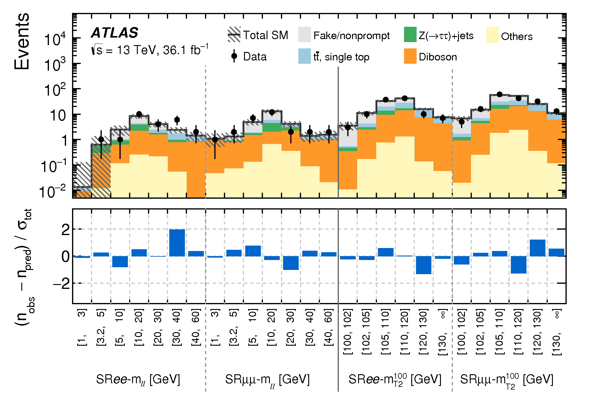
Figure 09: Comparison of observed and expected event yields after the exclusion fit with the signal strength parameter set to zero in the exclusive signal regions. Background processes containing fewer than two prompt leptons are categorized as `Fake/nonprompt'. The category `Others' contains rare backgrounds from triboson, Higgs boson, and the remaining top-quark production processes listed in Table 1. Uncertainties in the background estimates include both the statistical and systematic uncertainties, where σ_tot denotes the total uncertainty. png (32kB) pdf (23kB)
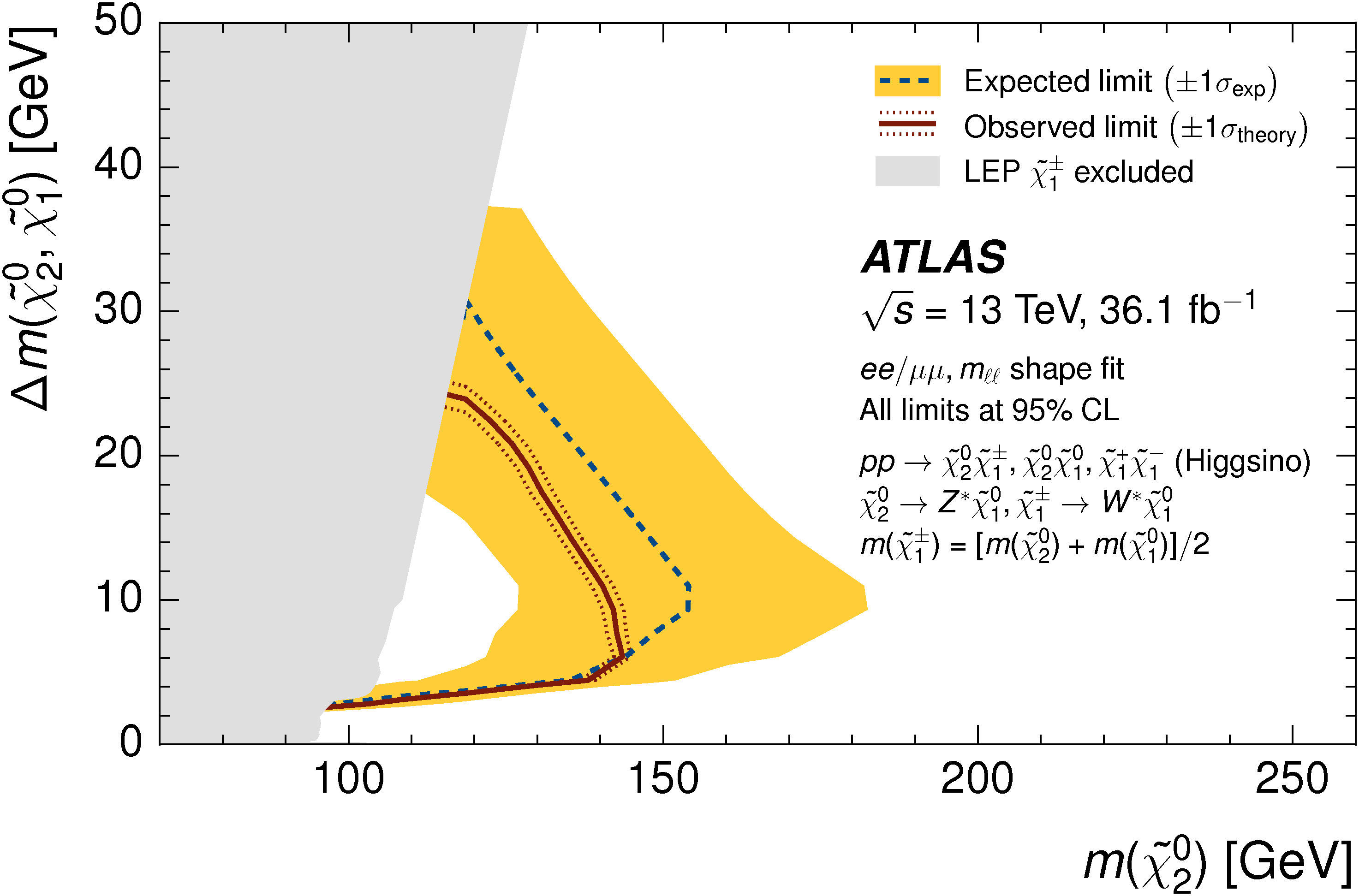
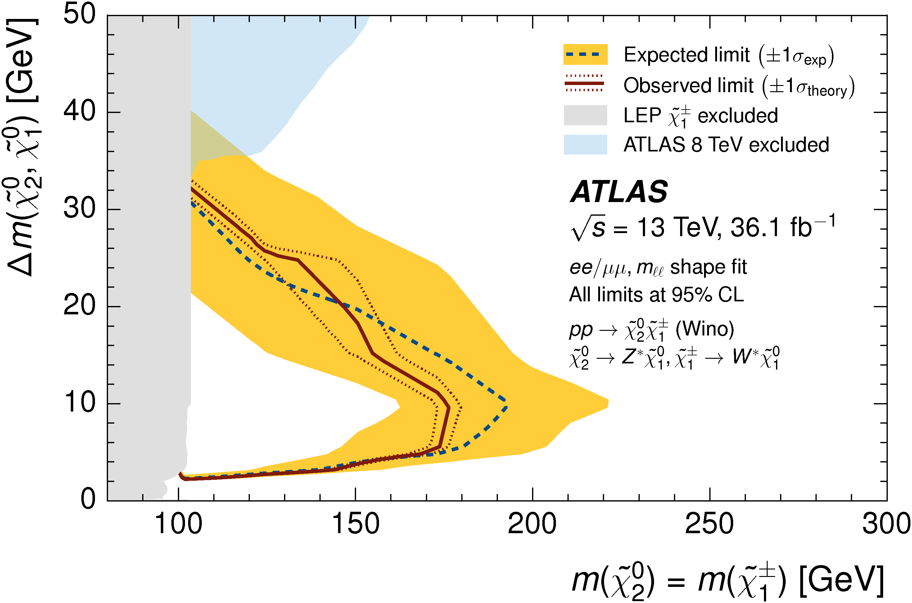
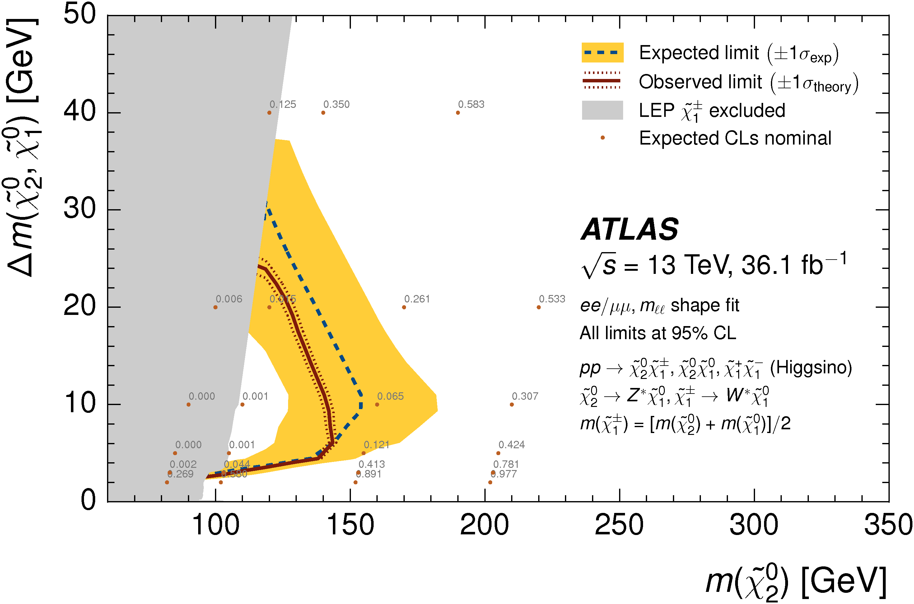
Figure 10a: Expected 95% CL exclusion sensitivity (blue dashed line) with pm1σ_exp (yellow band) from experimental systematic uncertainties and observed limits (red solid line) with pm1σ_theory (dotted red line) from signal cross-section uncertainties for simplified models of direct Higgsino (top) and wino (bottom) production. A fit of signals to the m_ℓℓ spectrum is used to derive the limit, which is projected into the Δ m(χ̃₂⁰, χ̃₁⁰) vs. m(χ̃₂⁰) plane. For Higgsino production, the chargino χ̃₁^pm mass is assumed to be halfway between the two lightest neutralino masses, while m(χ̃₂⁰) = m(χ̃₁^pm) is assumed for the wino--bino model. The gray regions denote the lower chargino mass limit from LEP. The blue region in the lower plot indicates the limit from the 2ℓ+3ℓ combination of ATLAS Run 1. png (54kB) pdf (256kB)
Figure 10b: Expected 95% CL exclusion sensitivity (blue dashed line) with pm1σ_exp (yellow band) from experimental systematic uncertainties and observed limits (red solid line) with pm1σ_theory (dotted red line) from signal cross-section uncertainties for simplified models of direct Higgsino (top) and wino (bottom) production. A fit of signals to the m_ℓℓ spectrum is used to derive the limit, which is projected into the Δ m(χ̃₂⁰, χ̃₁⁰) vs. m(χ̃₂⁰) plane. For Higgsino production, the chargino χ̃₁^pm mass is assumed to be halfway between the two lightest neutralino masses, while m(χ̃₂⁰) = m(χ̃₁^pm) is assumed for the wino--bino model. The gray regions denote the lower chargino mass limit from LEP. The blue region in the lower plot indicates the limit from the 2ℓ+3ℓ combination of ATLAS Run 1. png (57kB) pdf (261kB)
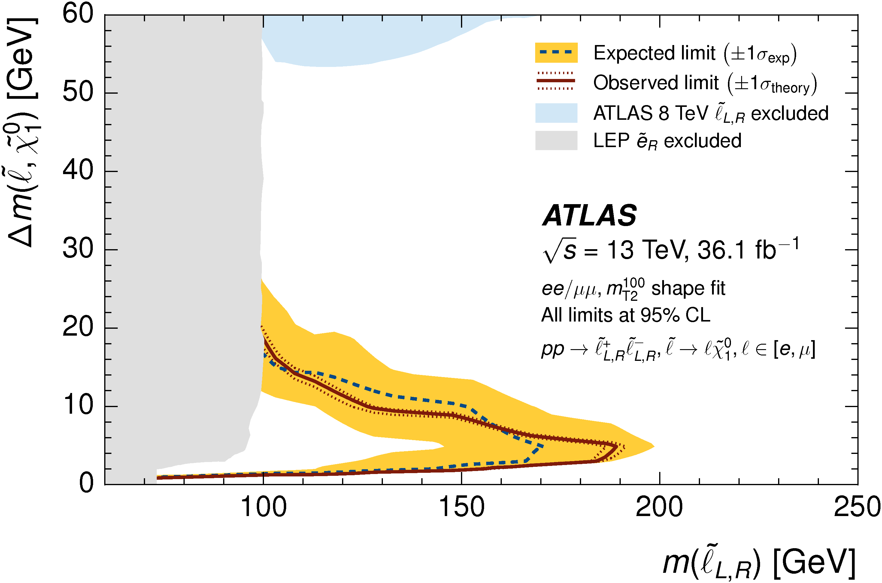
Figure 11: Expected 95% CL exclusion sensitivity (blue dashed line) with ± 1 σ_exp (yellow band) from experimental systematic uncertainties and observed limits (red solid line) with ± 1 σ_theory (dotted red line) from signal cross-section uncertainties for simplified models of direct slepton production. A fit of slepton signals to the m_T2¹⁰⁰ spectrum is used to derive the limit, which is projected into the Δ m(ℓ̃, χ̃₁⁰) vs. m(ℓ̃) plane. Slepton ℓ̃ refers to the scalar partners of left- and right-handed electrons and muons, which are assumed to be fourfold mass degenerate m(ẽ_L) = m(ẽ_R) = m(μ̃_L) = m(μ̃_R). The gray region is the ẽ_R limit from LEP, while the blue region is the fourfold mass degenerate slepton limit from ATLAS Run 1. png (51kB) pdf (261kB)
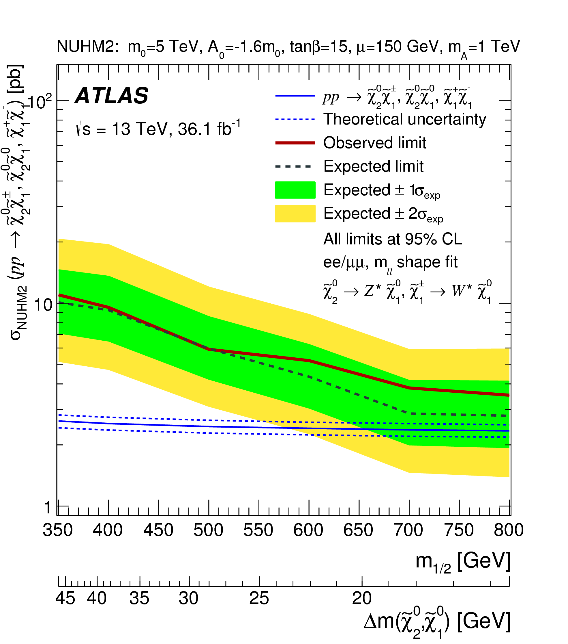
Figure 12: Observed and expected 95% CL cross-section upper limits as a function of the universal gaugino mass m_1/2 for the NUHM2 model. The green and yellow bands around the expected limit indicate the ± 1σ and ± 2σ uncertainties, respectively. The expected signal production cross-sections as well as the associated uncertainty are indicated with the blue solid and dashed lines. The lower x-axis indicates the difference between the χ̃₂⁰ and χ̃₁⁰ masses for different values of m_1/2. A fit of signals to the m_ℓℓ spectrum is used to derive this limit. png (142kB) eps (27kB) pdf (16kB)
Tables
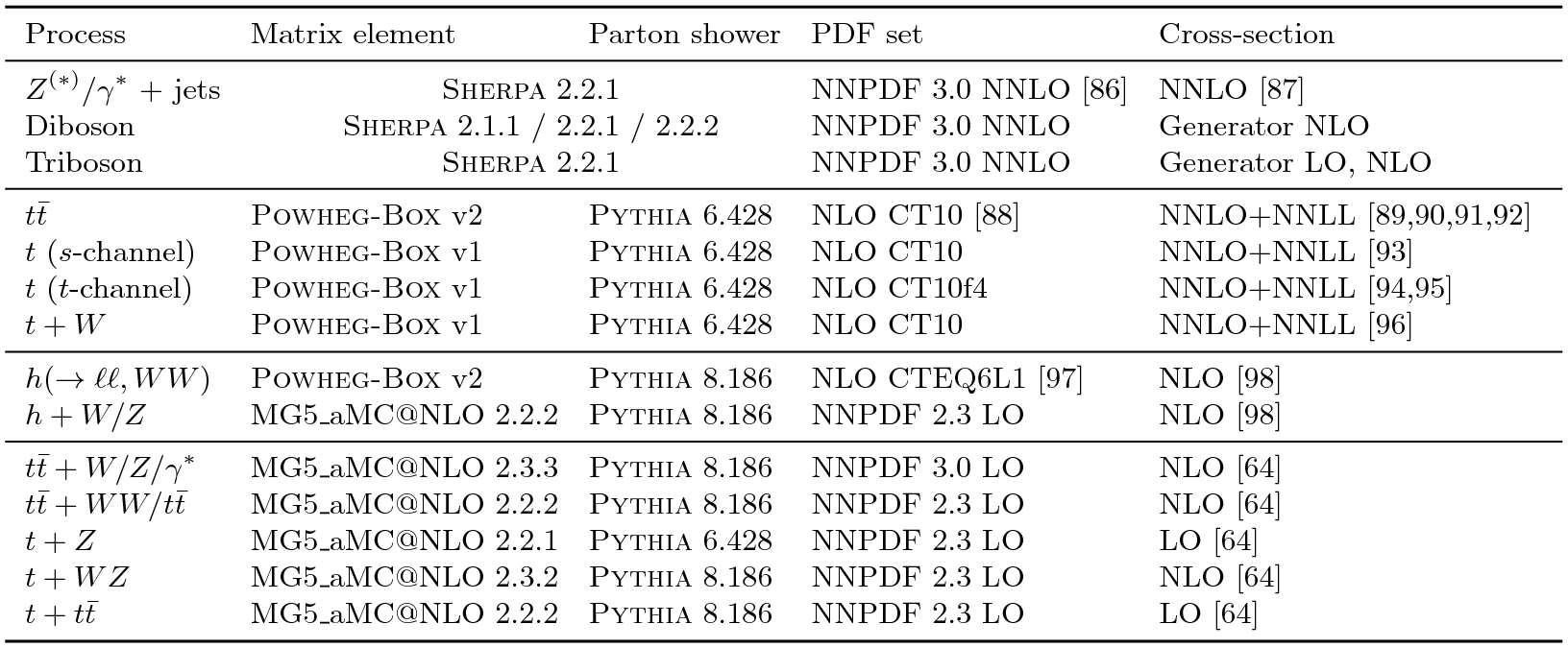
Table 01: Simulated samples of Standard Model background processes. The PDF set refers to that used for the matrix element. png (37kB) pdf (60kB)
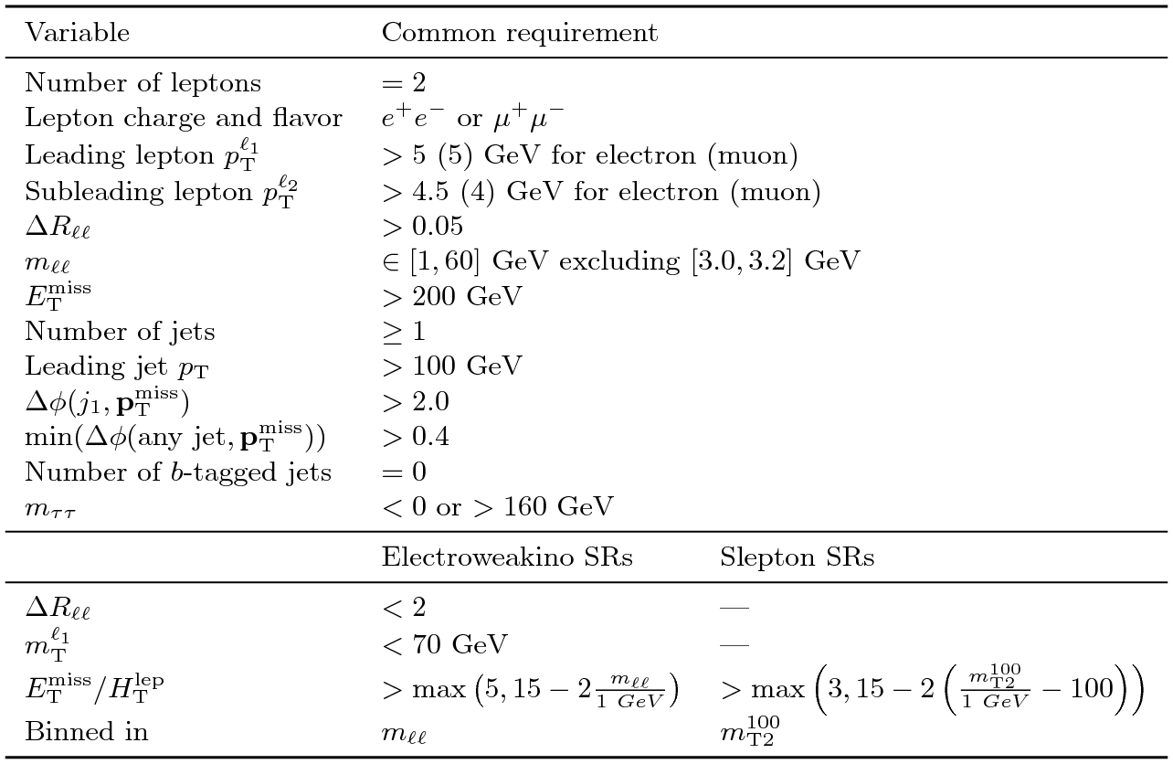
Table 02: Summary of event selection criteria. The binning scheme used to define the final signal regions is shown in Table 3. Signal leptons and signal jets are used when applying all requirements. png (33kB) pdf (90kB)
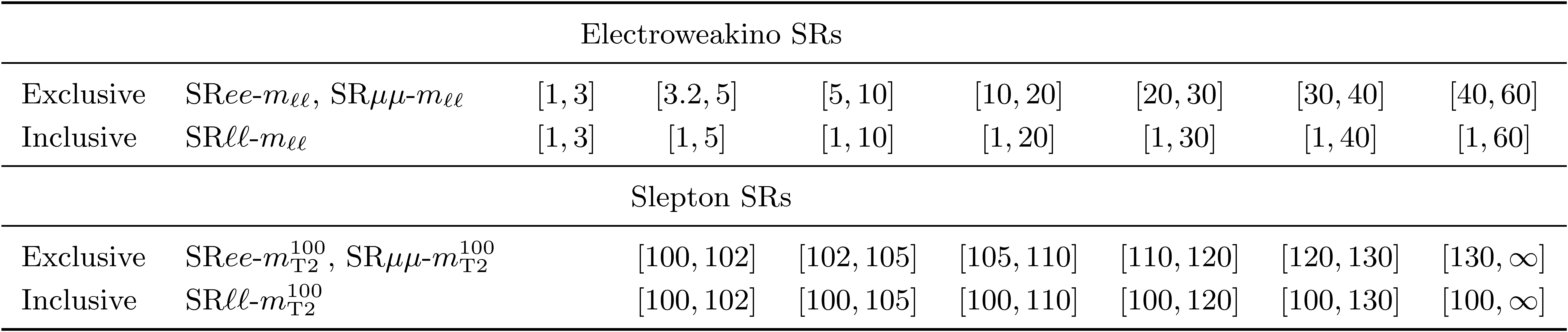
Table 03: Signal region binning for the electroweakino and slepton SRs. Each SR is defined by the lepton flavor (ee, μμ, or ℓℓ for both) and a range of m_ℓℓ (for electroweakino SRs) or m_T2¹⁰⁰ (for slepton SRs) in GeV. The inclusive bins are used to set model-independent limits, while the exclusive bins are used to derive exclusion limits on signal models. png (80kB) pdf (45kB)
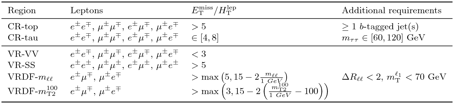
Table 04: Definition of control and validation regions. The common selection criteria in Table 2 are implied unless otherwise specified. png (19kB) pdf (81kB)
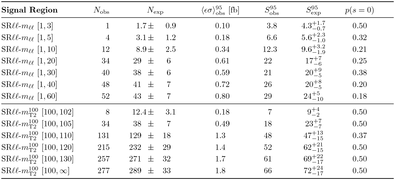
Table 05: Left to right: The first two columns present observed (N_obs) and expected (N_exp) event yields in the inclusive signal regions. The latter are obtained by the background-only fit of the control regions, and the errors include both statistical and systematic uncertainties. The next two columns show the observed 95% CL upper limits on the visible cross-section (⟨εσ⟩_obs⁹⁵) and on the number of signal events (S_obs⁹⁵). The fifth column (S_exp⁹⁵) shows what the 95% CL upper limit on the number of signal events would be, given an observed number of events equal to the expected number (and pm1σ deviations from the expectation) of background events. The last column indicates the discovery p-value (p(s = 0)), which is capped at 0.5. png (54kB) pdf (66kB)
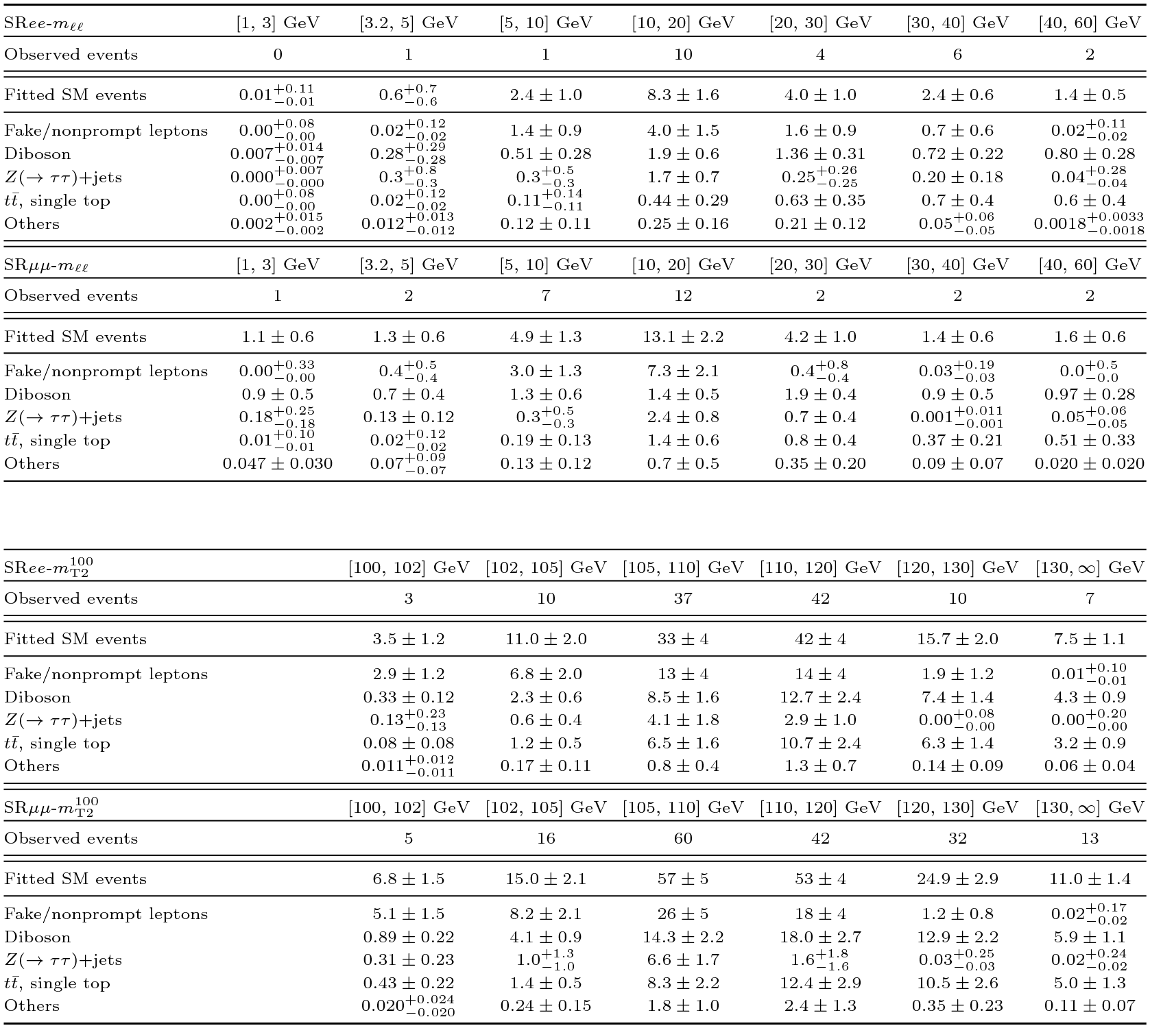
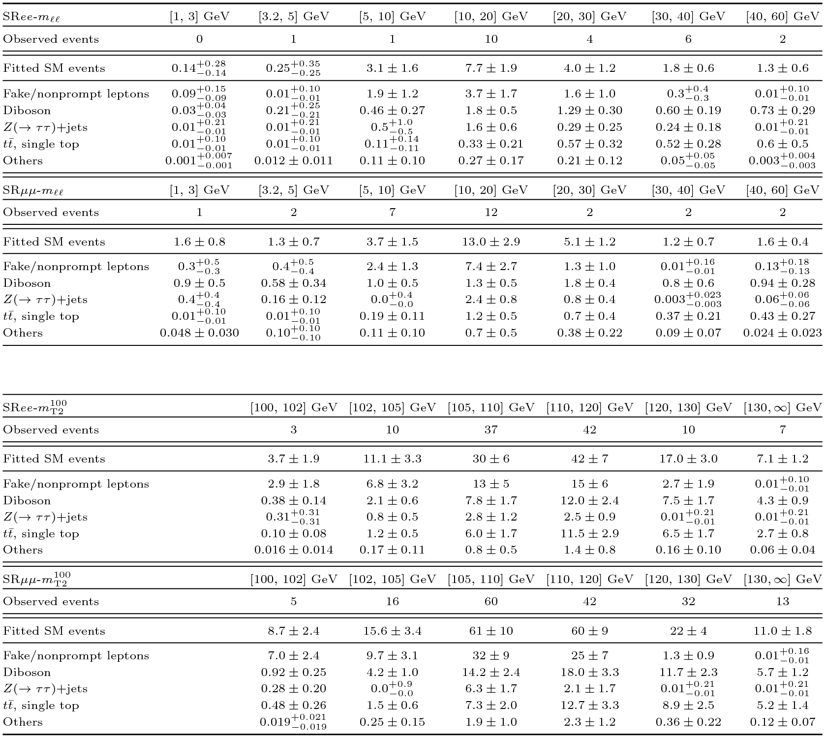
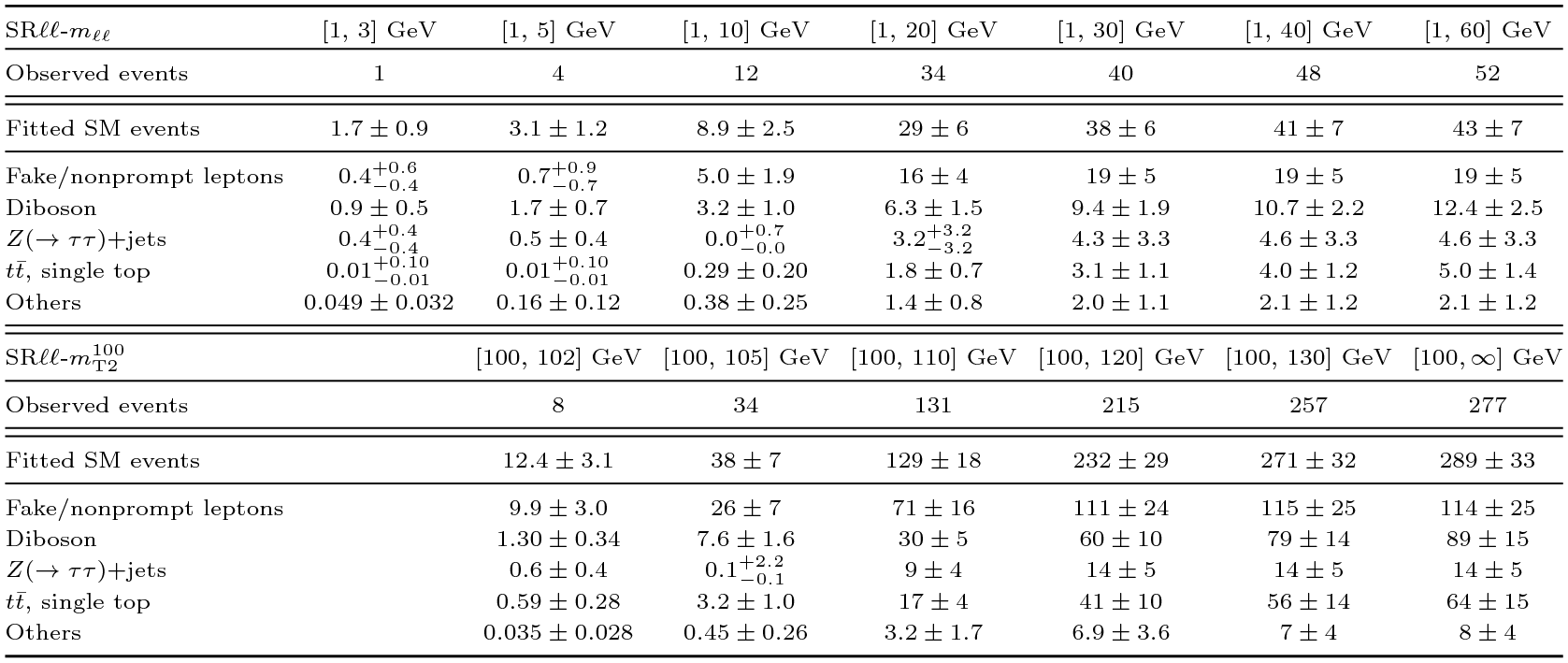
Table 06: Observed event yields and exclusion fit results with the signal strength parameter set to zero for the exclusive electroweakino and slepton signal regions. Background processes containing fewer than two prompt leptons are categorized as `Fake/nonprompt'. The category `Others' contains rare backgrounds from triboson, Higgs boson, and the remaining top-quark production processes listed in Table 1. Uncertainties in the fitted background estimates combine statistical and systematic uncertainties. png (85kB) pdf (58kB)
Auxiliary figures and tables
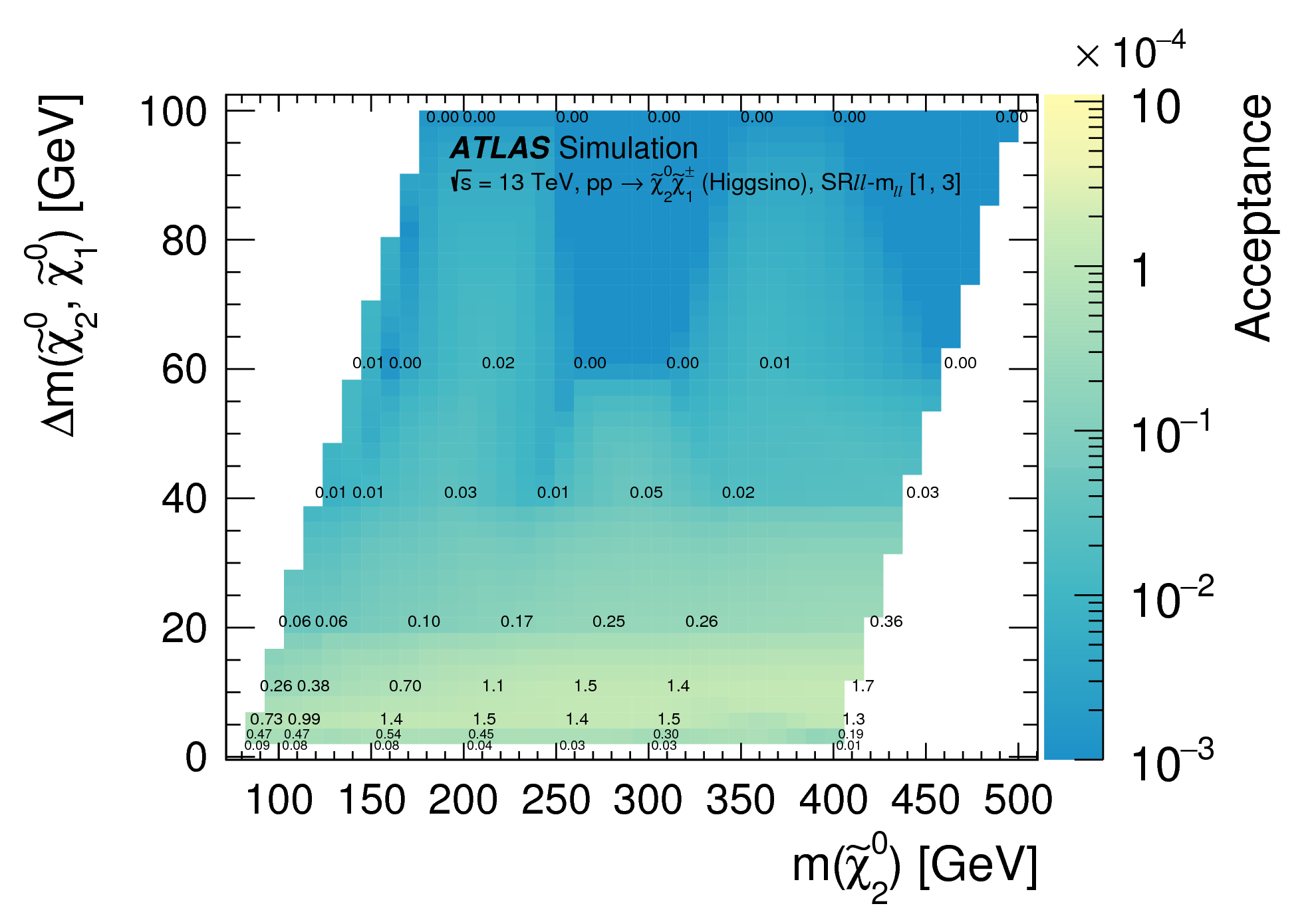
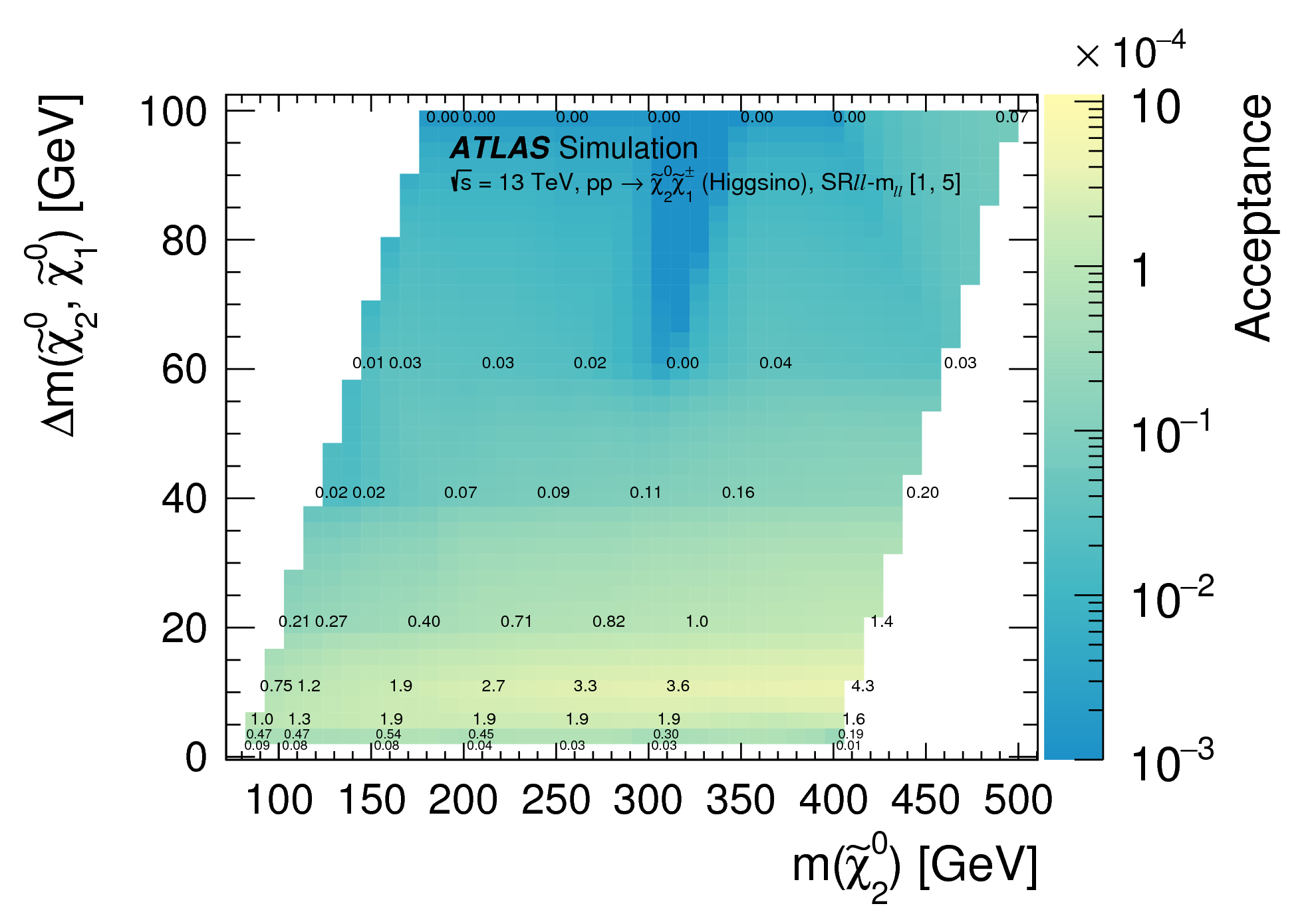
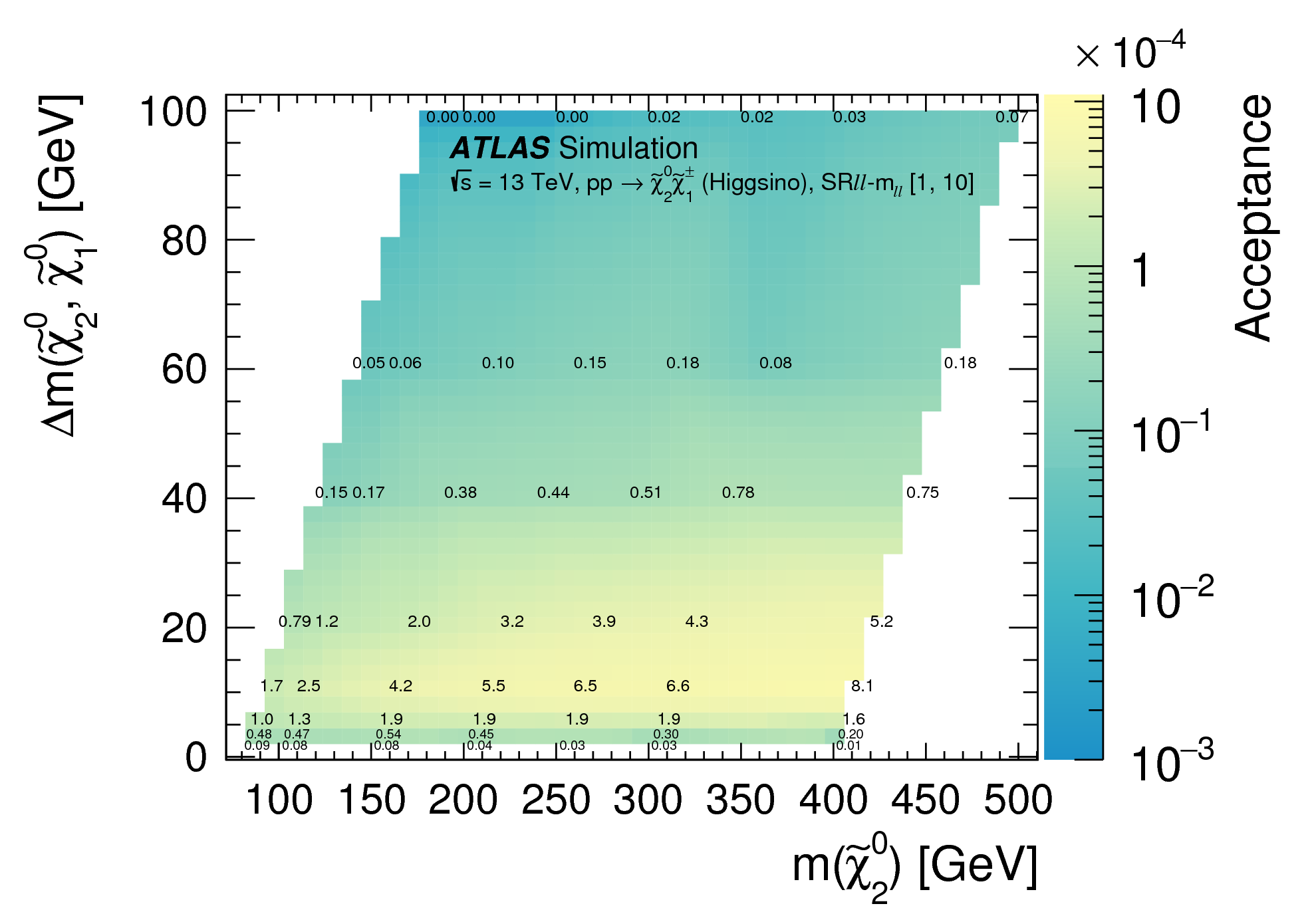
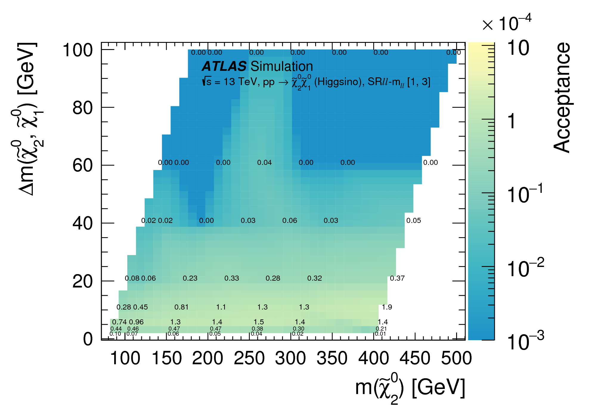
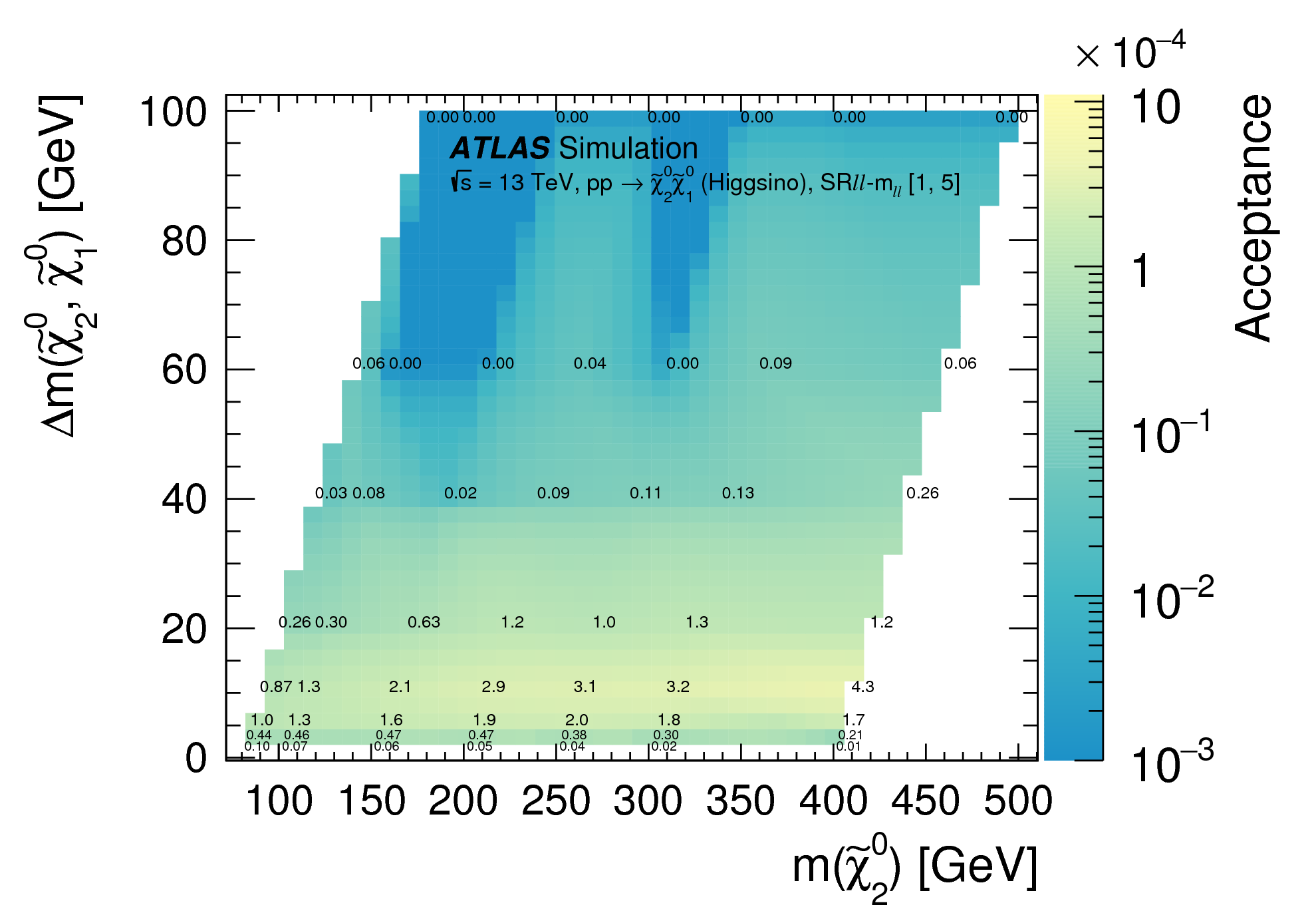
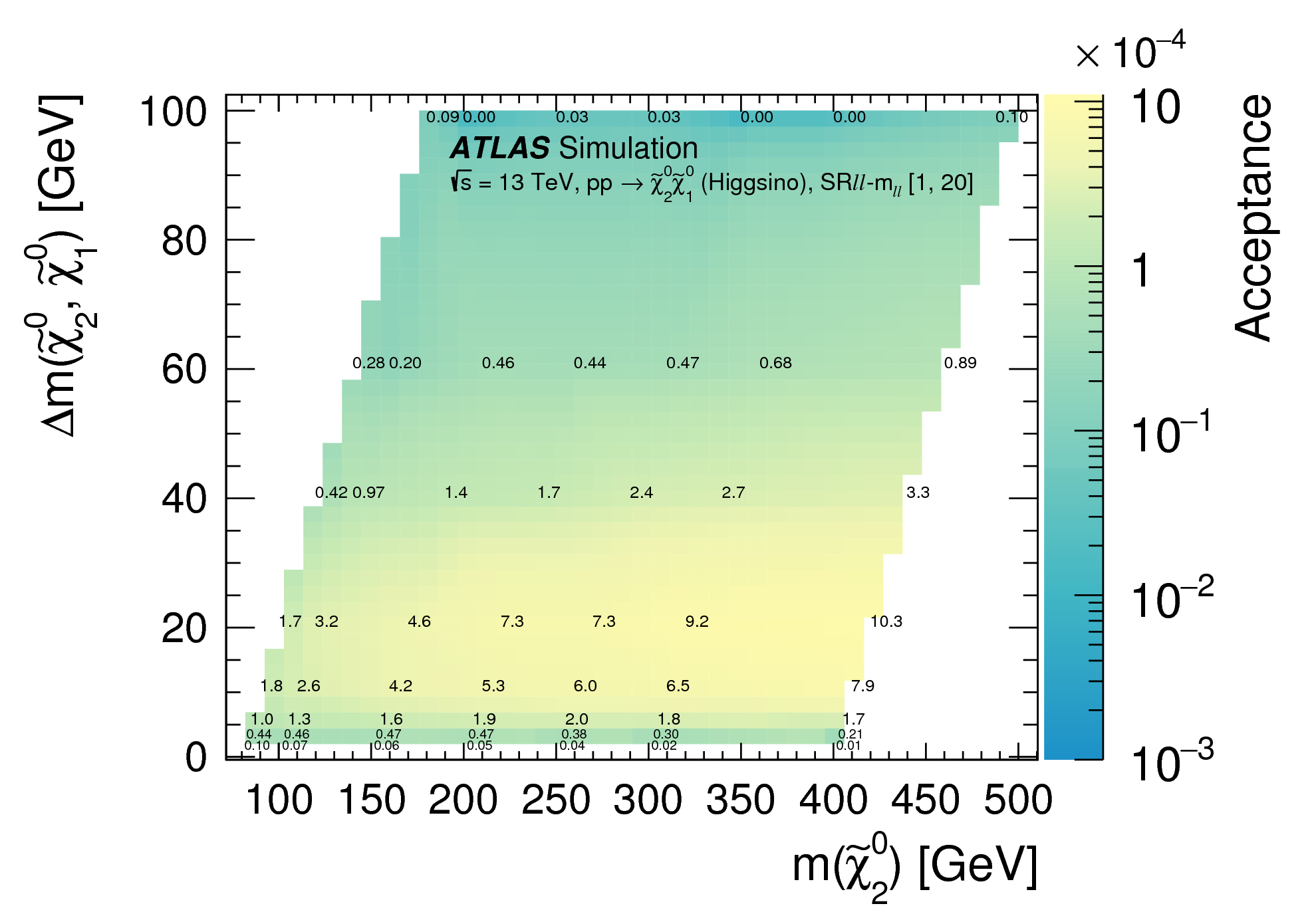
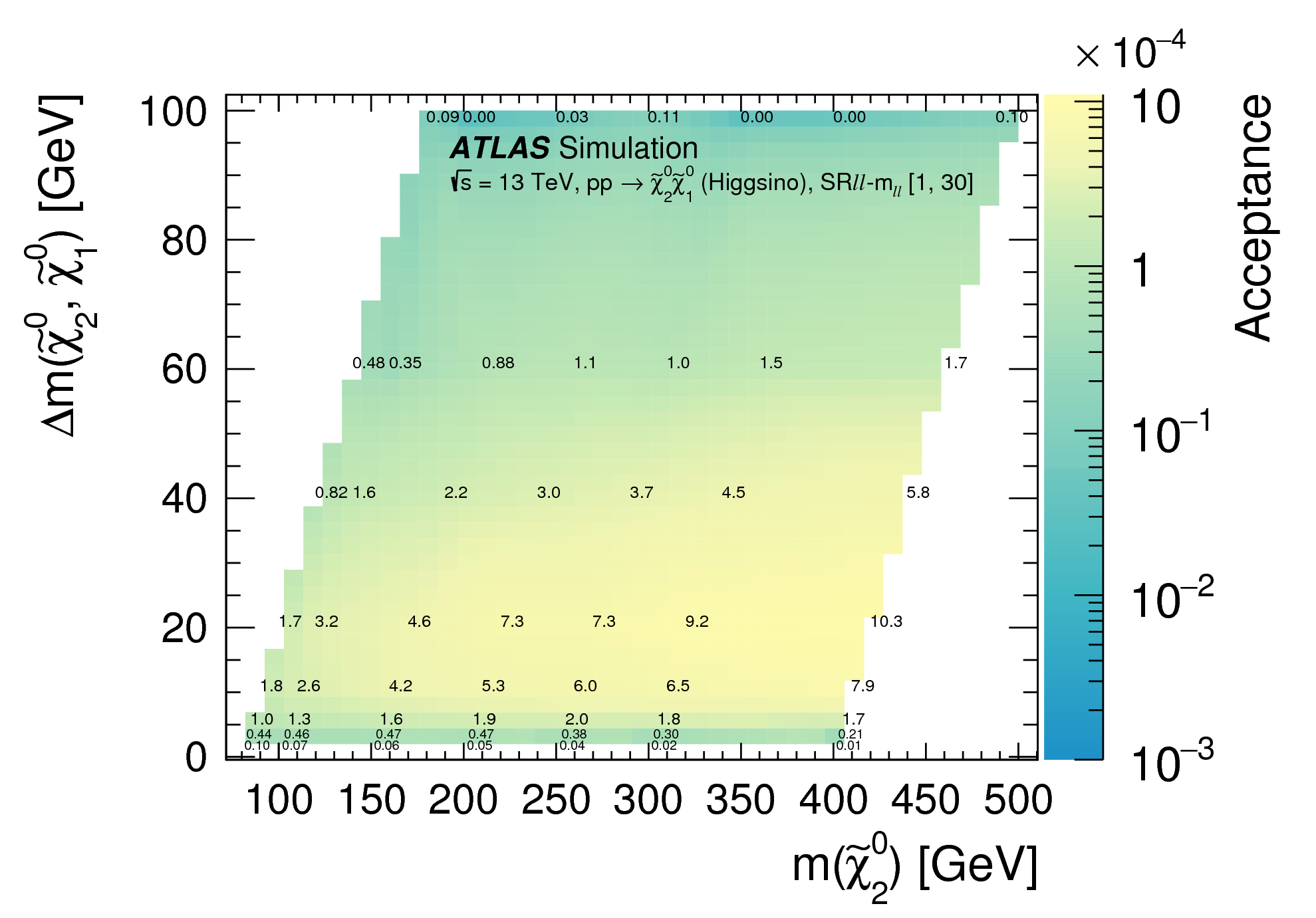
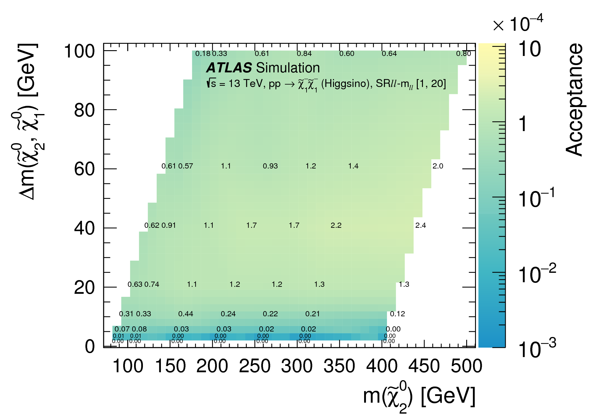
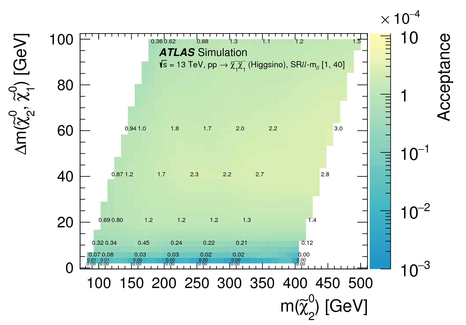
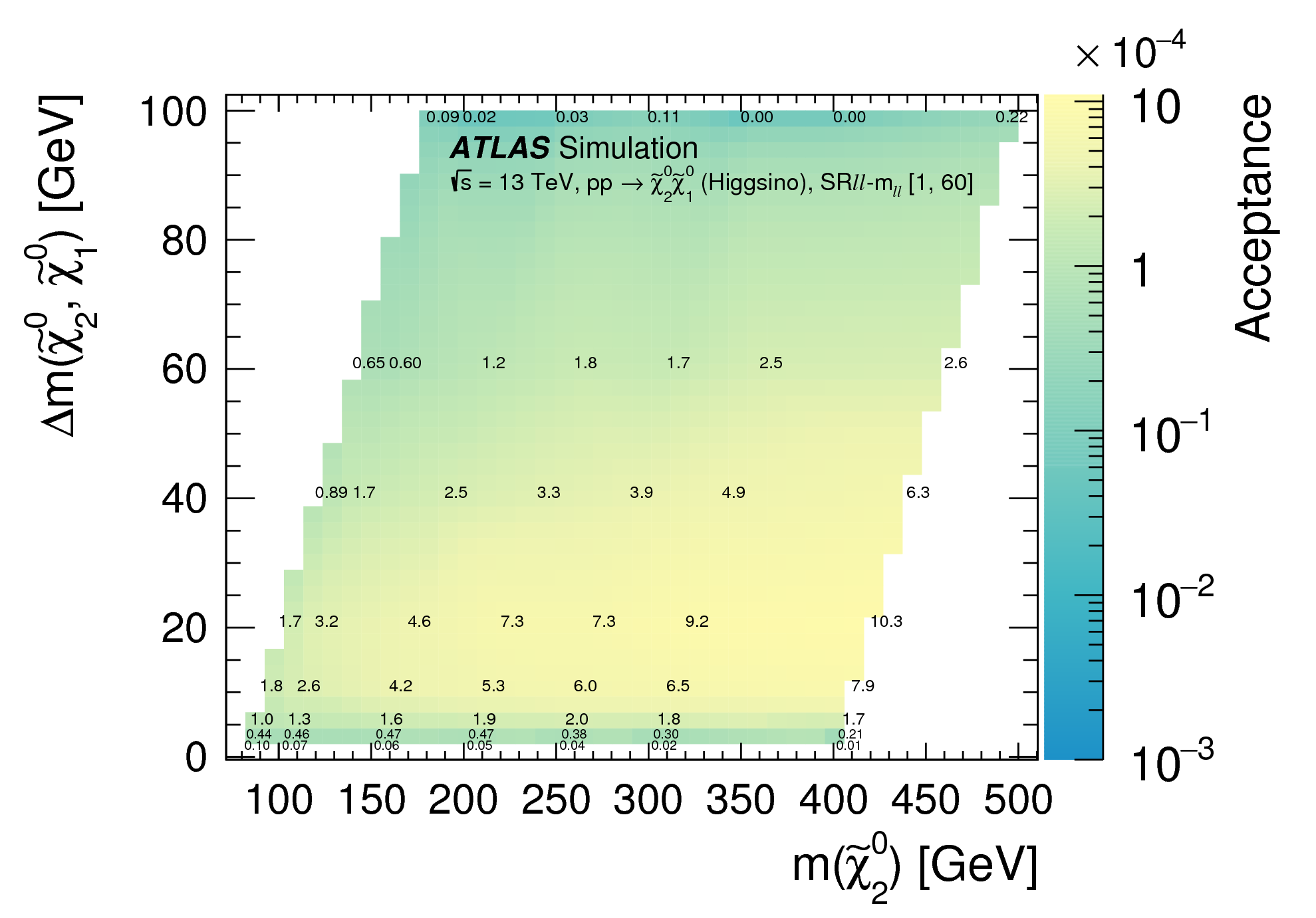
Figure 01a: Truth acceptances for the Higgsino χ̃₂⁰χ̃₁^± production process in the inclusive SRℓℓ-m_ℓℓ regions. Numbers overlaid on the mass planes are the acceptance × 10⁴. png (127kB) pdf (36kB)
Figure 01b: Truth acceptances for the Higgsino χ̃₂⁰χ̃₁^± production process in the inclusive SRℓℓ-m_ℓℓ regions. Numbers overlaid on the mass planes are the acceptance × 10⁴. png (129kB) pdf (37kB)
Figure 01c: Truth acceptances for the Higgsino χ̃₂⁰χ̃₁^± production process in the inclusive SRℓℓ-m_ℓℓ regions. Numbers overlaid on the mass planes are the acceptance × 10⁴. png (130kB) pdf (37kB)
Figure 01d: Truth acceptances for the Higgsino χ̃₂⁰χ̃₁^± production process in the inclusive SRℓℓ-m_ℓℓ regions. Numbers overlaid on the mass planes are the acceptance × 10⁴. png (127kB) pdf (37kB)
Figure 01e: Truth acceptances for the Higgsino χ̃₂⁰χ̃₁^± production process in the inclusive SRℓℓ-m_ℓℓ regions. Numbers overlaid on the mass planes are the acceptance × 10⁴. png (130kB) pdf (37kB)
Figure 01f: Truth acceptances for the Higgsino χ̃₂⁰χ̃₁^± production process in the inclusive SRℓℓ-m_ℓℓ regions. Numbers overlaid on the mass planes are the acceptance × 10⁴. png (128kB) pdf (36kB)
Figure 01g: Truth acceptances for the Higgsino χ̃₂⁰χ̃₁^± production process in the inclusive SRℓℓ-m_ℓℓ regions. Numbers overlaid on the mass planes are the acceptance × 10⁴. png (128kB) pdf (36kB)
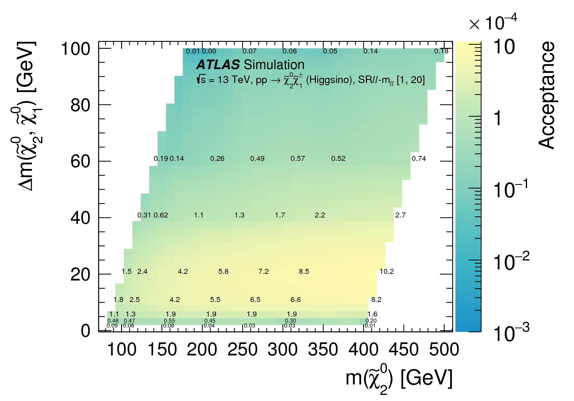
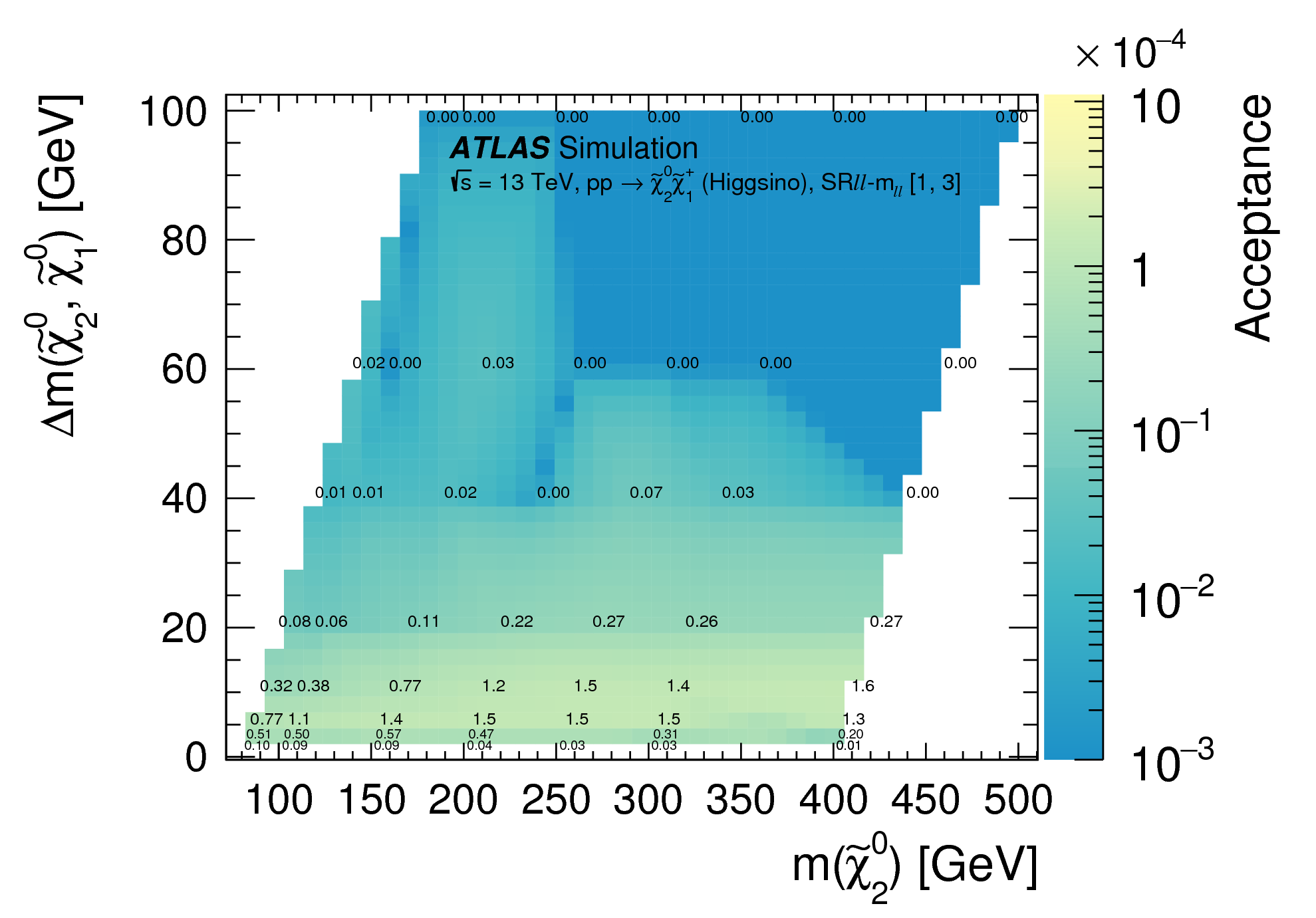
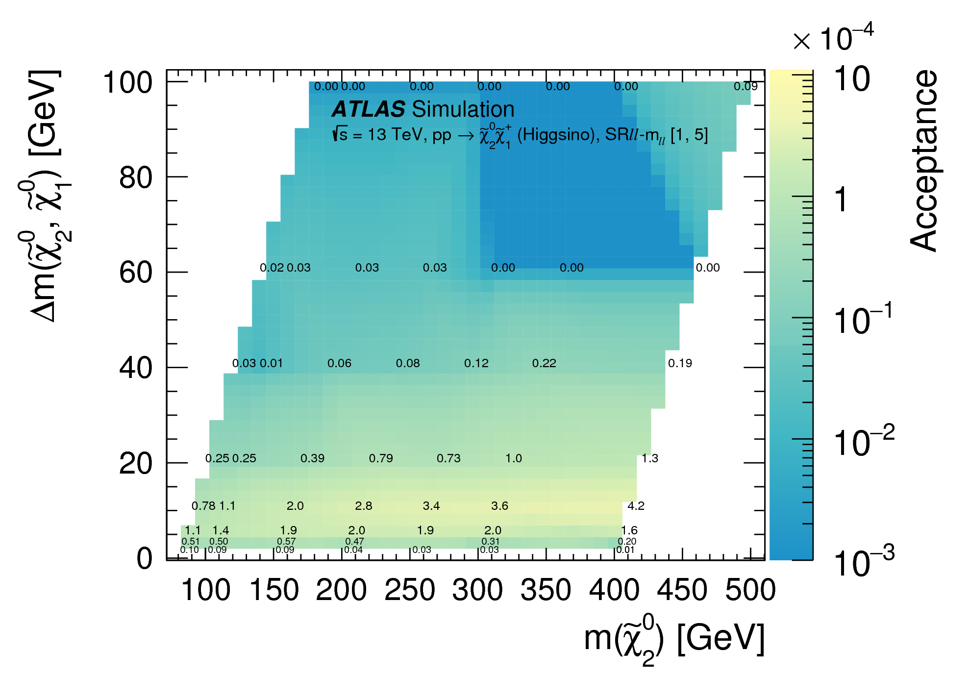
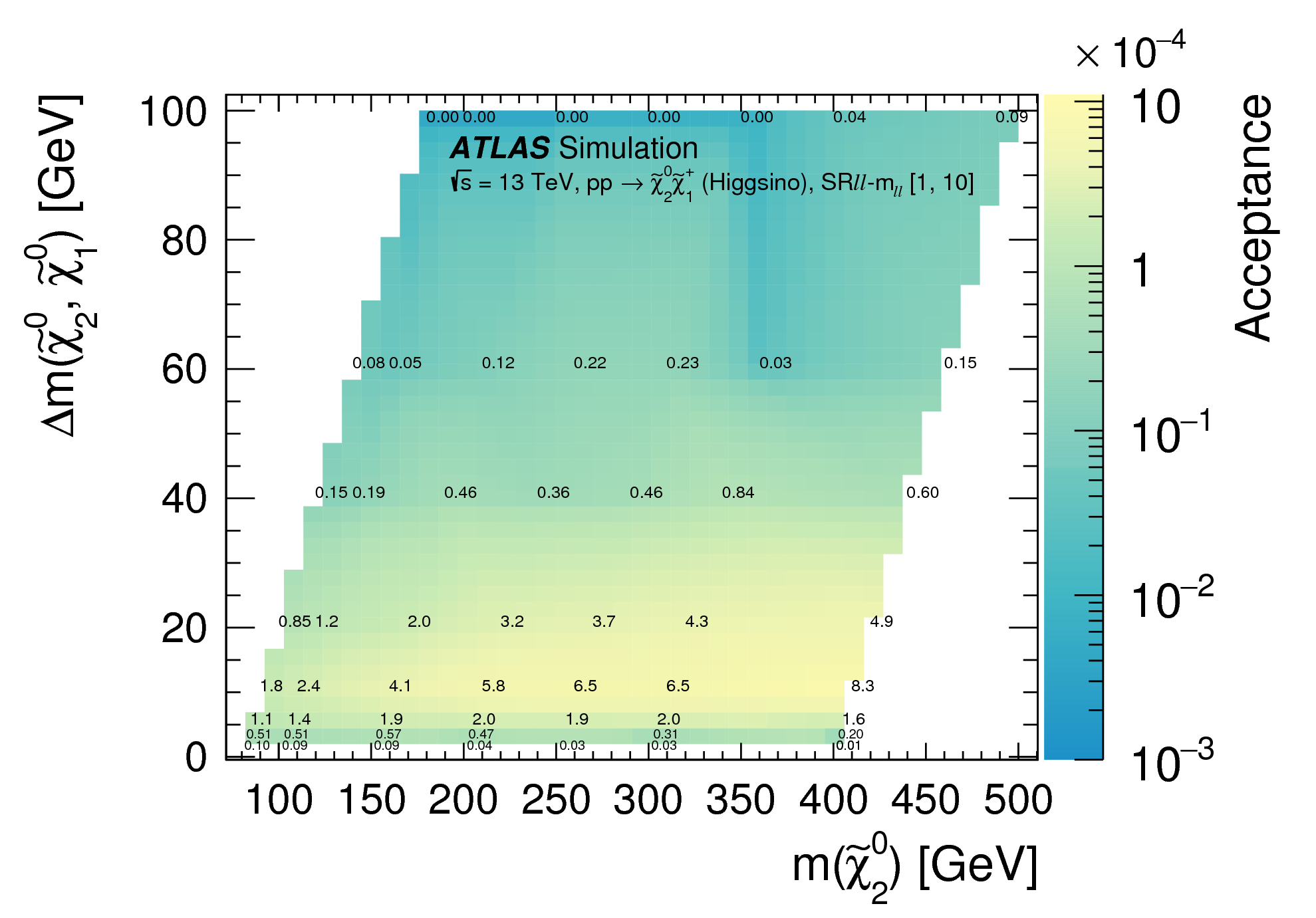
Figure 02a: Truth acceptances for the Higgsino χ̃₂⁰χ̃₁⁺ production process in the inclusive SRℓℓ-m_ℓℓ regions. Numbers overlaid on the mass planes are the acceptance × 10⁴. png (120kB) pdf (36kB)
Figure 02b: Truth acceptances for the Higgsino χ̃₂⁰χ̃₁⁺ production process in the inclusive SRℓℓ-m_ℓℓ regions. Numbers overlaid on the mass planes are the acceptance × 10⁴. png (126kB) pdf (36kB)
Figure 02c: Truth acceptances for the Higgsino χ̃₂⁰χ̃₁⁺ production process in the inclusive SRℓℓ-m_ℓℓ regions. Numbers overlaid on the mass planes are the acceptance × 10⁴. png (129kB) pdf (37kB)
Figure 02d: Truth acceptances for the Higgsino χ̃₂⁰χ̃₁⁺ production process in the inclusive SRℓℓ-m_ℓℓ regions. Numbers overlaid on the mass planes are the acceptance × 10⁴. png (127kB) pdf (37kB)
Figure 02e: Truth acceptances for the Higgsino χ̃₂⁰χ̃₁⁺ production process in the inclusive SRℓℓ-m_ℓℓ regions. Numbers overlaid on the mass planes are the acceptance × 10⁴. png (127kB) pdf (36kB)
Figure 02f: Truth acceptances for the Higgsino χ̃₂⁰χ̃₁⁺ production process in the inclusive SRℓℓ-m_ℓℓ regions. Numbers overlaid on the mass planes are the acceptance × 10⁴. png (128kB) pdf (36kB)
Figure 02g: Truth acceptances for the Higgsino χ̃₂⁰χ̃₁⁺ production process in the inclusive SRℓℓ-m_ℓℓ regions. Numbers overlaid on the mass planes are the acceptance × 10⁴. png (128kB) pdf (36kB)
Figure 03a: Truth acceptances for the Higgsino χ̃₂⁰χ̃₁⁰ production process in the inclusive SRℓℓ-m_ℓℓ regions. Numbers overlaid on the mass planes are the acceptance × 10⁴. png (124kB) pdf (36kB)
Figure 03b: Truth acceptances for the Higgsino χ̃₂⁰χ̃₁⁰ production process in the inclusive SRℓℓ-m_ℓℓ regions. Numbers overlaid on the mass planes are the acceptance × 10⁴. png (128kB) pdf (37kB)
Figure 03c: Truth acceptances for the Higgsino χ̃₂⁰χ̃₁⁰ production process in the inclusive SRℓℓ-m_ℓℓ regions. Numbers overlaid on the mass planes are the acceptance × 10⁴. png (126kB) pdf (37kB)
Figure 03d: Truth acceptances for the Higgsino χ̃₂⁰χ̃₁⁰ production process in the inclusive SRℓℓ-m_ℓℓ regions. Numbers overlaid on the mass planes are the acceptance × 10⁴. png (128kB) pdf (36kB)
Figure 03e: Truth acceptances for the Higgsino χ̃₂⁰χ̃₁⁰ production process in the inclusive SRℓℓ-m_ℓℓ regions. Numbers overlaid on the mass planes are the acceptance × 10⁴. png (126kB) pdf (36kB)
Figure 03f: Truth acceptances for the Higgsino χ̃₂⁰χ̃₁⁰ production process in the inclusive SRℓℓ-m_ℓℓ regions. Numbers overlaid on the mass planes are the acceptance × 10⁴. png (125kB) pdf (36kB)
Figure 03g: Truth acceptances for the Higgsino χ̃₂⁰χ̃₁⁰ production process in the inclusive SRℓℓ-m_ℓℓ regions. Numbers overlaid on the mass planes are the acceptance × 10⁴. png (127kB) pdf (36kB)
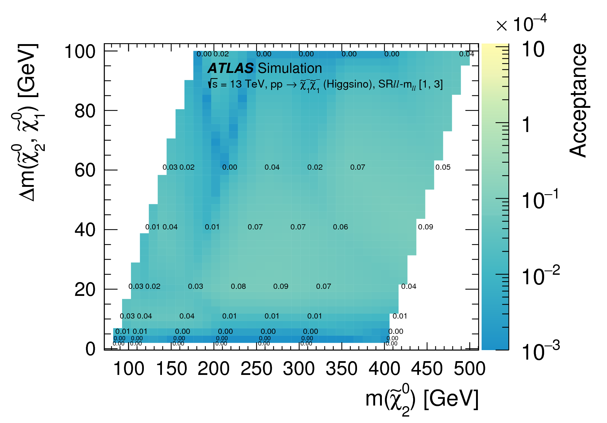
Figure 04a: Truth acceptances for the Higgsino χ̃₁⁺χ̃₁^- production process in the inclusive SRℓℓ-m_ℓℓ regions. Numbers overlaid on the mass planes are the acceptance × 10⁴. png (130kB) pdf (36kB)
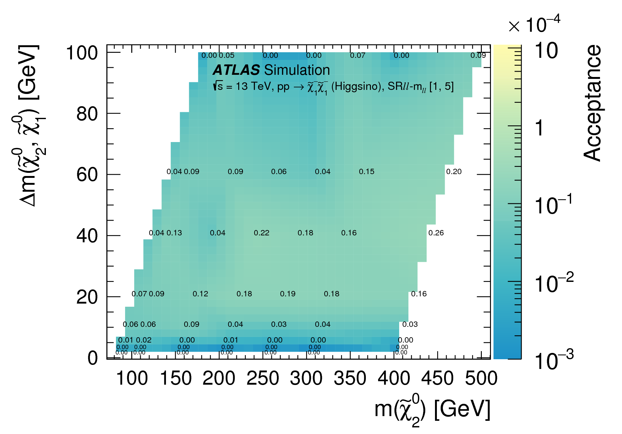
Figure 04b: Truth acceptances for the Higgsino χ̃₁⁺χ̃₁^- production process in the inclusive SRℓℓ-m_ℓℓ regions. Numbers overlaid on the mass planes are the acceptance × 10⁴. png (133kB) pdf (36kB)
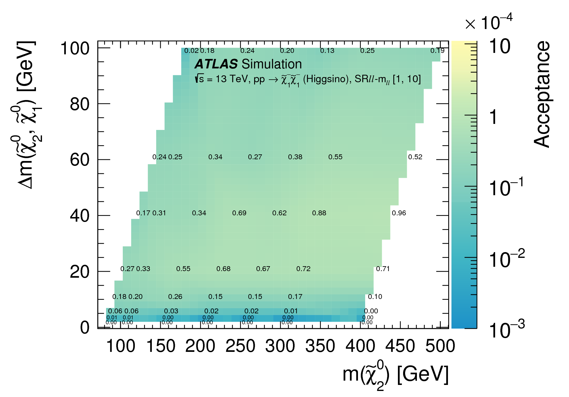
Figure 04c: Truth acceptances for the Higgsino χ̃₁⁺χ̃₁^- production process in the inclusive SRℓℓ-m_ℓℓ regions. Numbers overlaid on the mass planes are the acceptance × 10⁴. png (132kB) pdf (35kB)
Figure 04d: Truth acceptances for the Higgsino χ̃₁⁺χ̃₁^- production process in the inclusive SRℓℓ-m_ℓℓ regions. Numbers overlaid on the mass planes are the acceptance × 10⁴. png (124kB) pdf (35kB)
Figure 04e: Truth acceptances for the Higgsino χ̃₁⁺χ̃₁^- production process in the inclusive SRℓℓ-m_ℓℓ regions. Numbers overlaid on the mass planes are the acceptance × 10⁴. png (125kB) pdf (35kB)
Figure 04f: Truth acceptances for the Higgsino χ̃₁⁺χ̃₁^- production process in the inclusive SRℓℓ-m_ℓℓ regions. Numbers overlaid on the mass planes are the acceptance × 10⁴. png (124kB) pdf (35kB)
Figure 04g: Truth acceptances for the Higgsino χ̃₁⁺χ̃₁^- production process in the inclusive SRℓℓ-m_ℓℓ regions. Numbers overlaid on the mass planes are the acceptance × 10⁴. png (124kB) pdf (35kB)
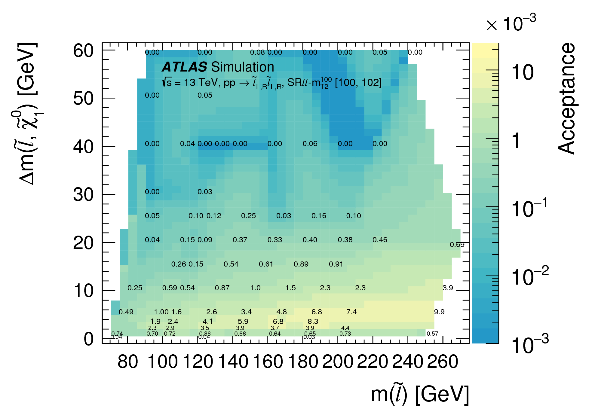
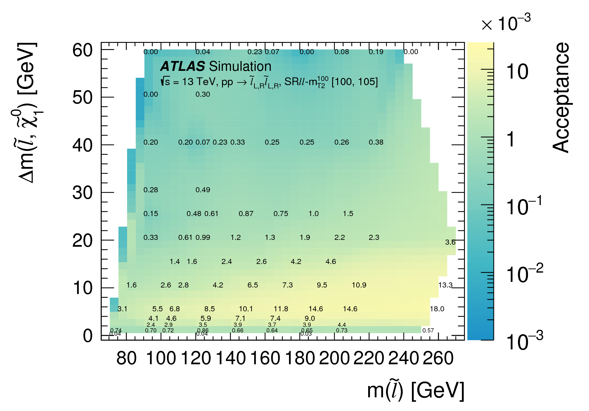
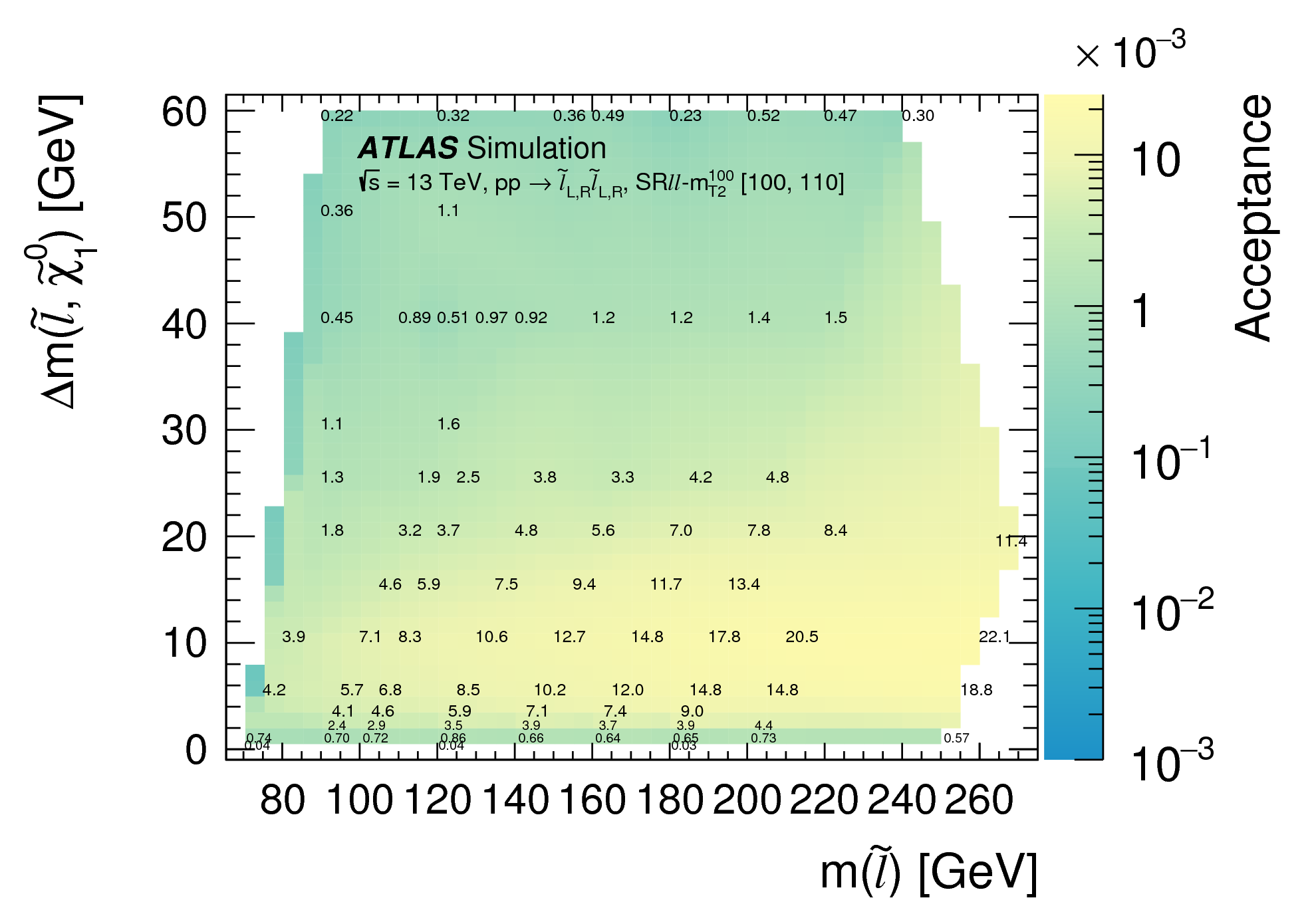
Figure 05a: Truth acceptances for the ℓ̃ℓ̃ production in the inclusive SRℓℓ-m_T2¹⁰⁰ regions. Numbers overlaid on the mass planes are the acceptance × 10³. png (142kB) pdf (23kB)
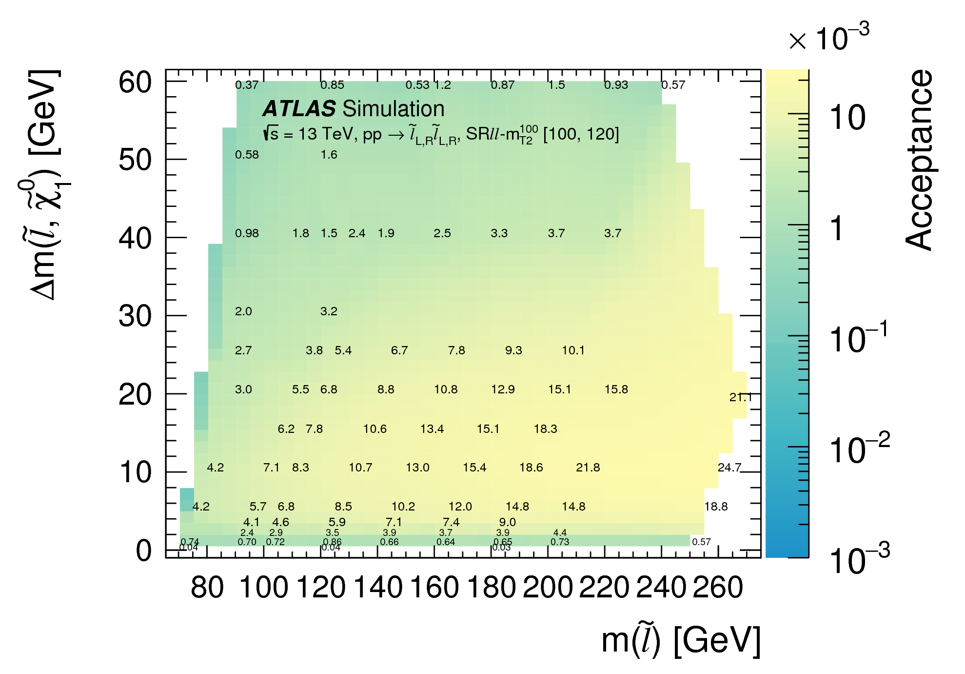
Figure 05b: Truth acceptances for the ℓ̃ℓ̃ production in the inclusive SRℓℓ-m_T2¹⁰⁰ regions. Numbers overlaid on the mass planes are the acceptance × 10³. png (153kB) pdf (39kB)
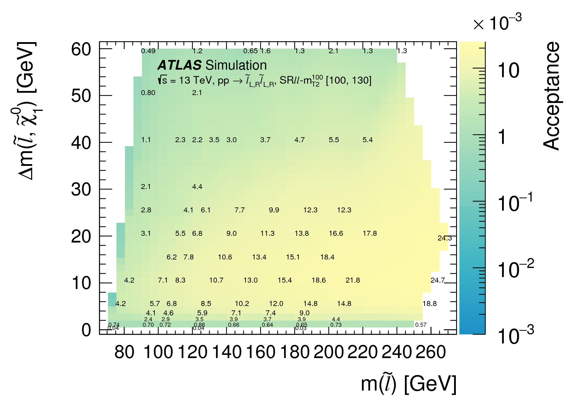
Figure 05c: Truth acceptances for the ℓ̃ℓ̃ production in the inclusive SRℓℓ-m_T2¹⁰⁰ regions. Numbers overlaid on the mass planes are the acceptance × 10³. png (147kB) pdf (38kB)
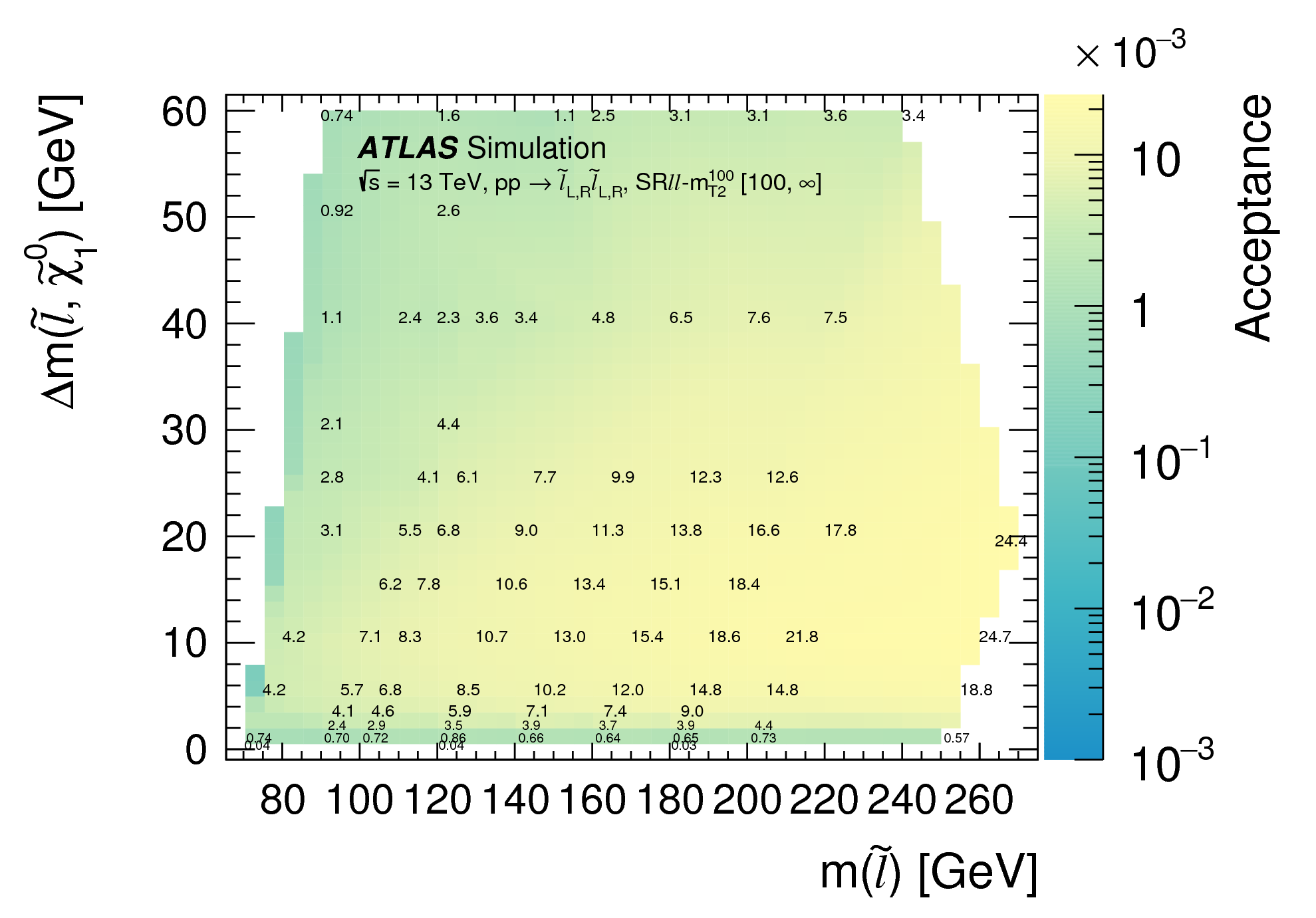
Figure 05d: Truth acceptances for the ℓ̃ℓ̃ production in the inclusive SRℓℓ-m_T2¹⁰⁰ regions. Numbers overlaid on the mass planes are the acceptance × 10³. png (149kB) pdf (38kB)
Figure 05e: Truth acceptances for the ℓ̃ℓ̃ production in the inclusive SRℓℓ-m_T2¹⁰⁰ regions. Numbers overlaid on the mass planes are the acceptance × 10³. png (145kB) pdf (38kB)
Figure 05f: Truth acceptances for the ℓ̃ℓ̃ production in the inclusive SRℓℓ-m_T2¹⁰⁰ regions. Numbers overlaid on the mass planes are the acceptance × 10³. png (145kB) pdf (38kB)
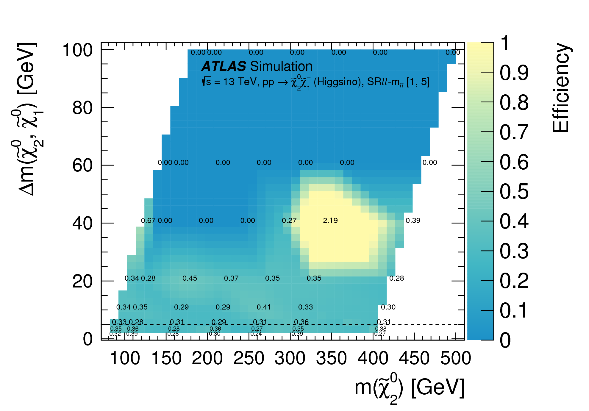
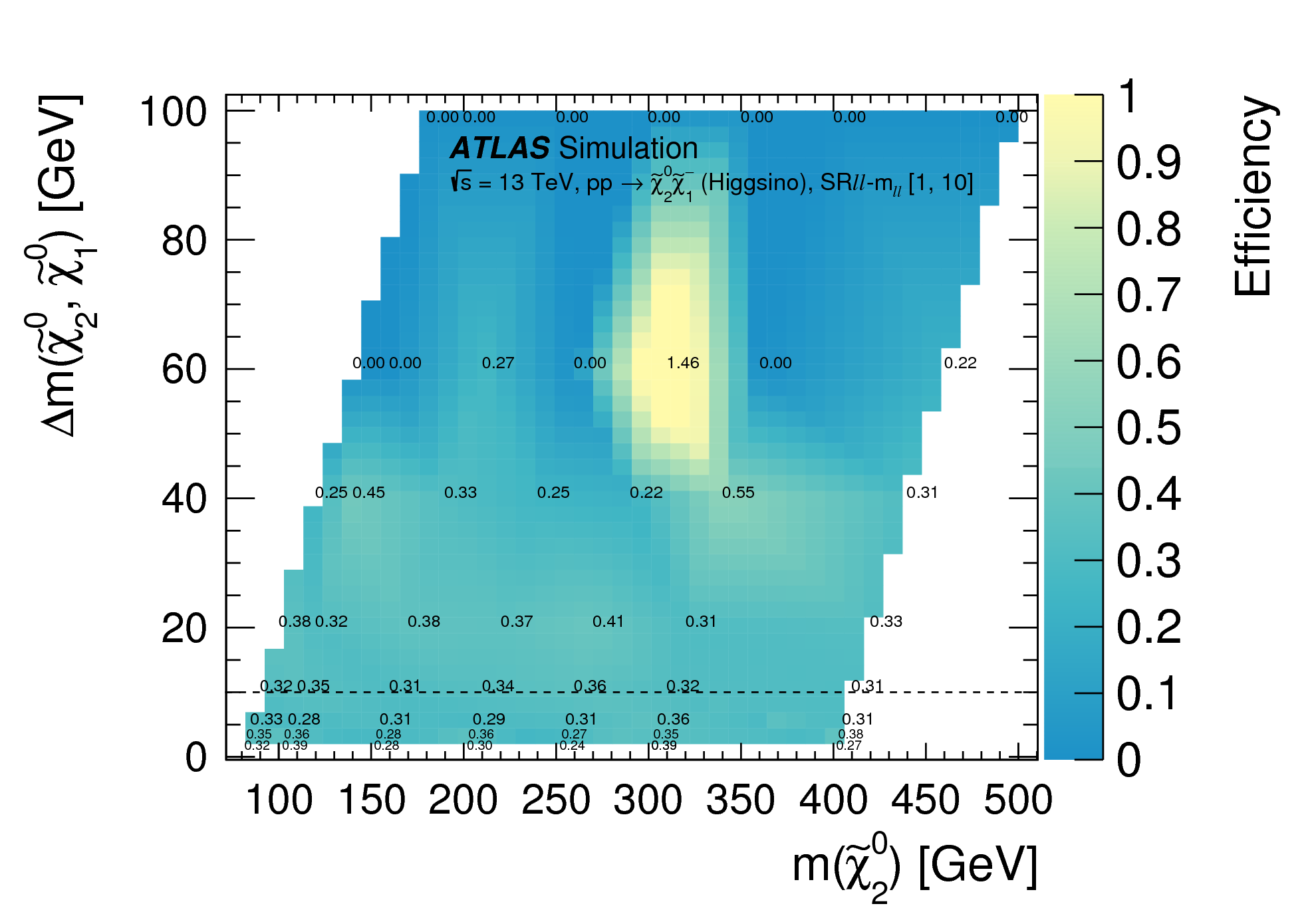
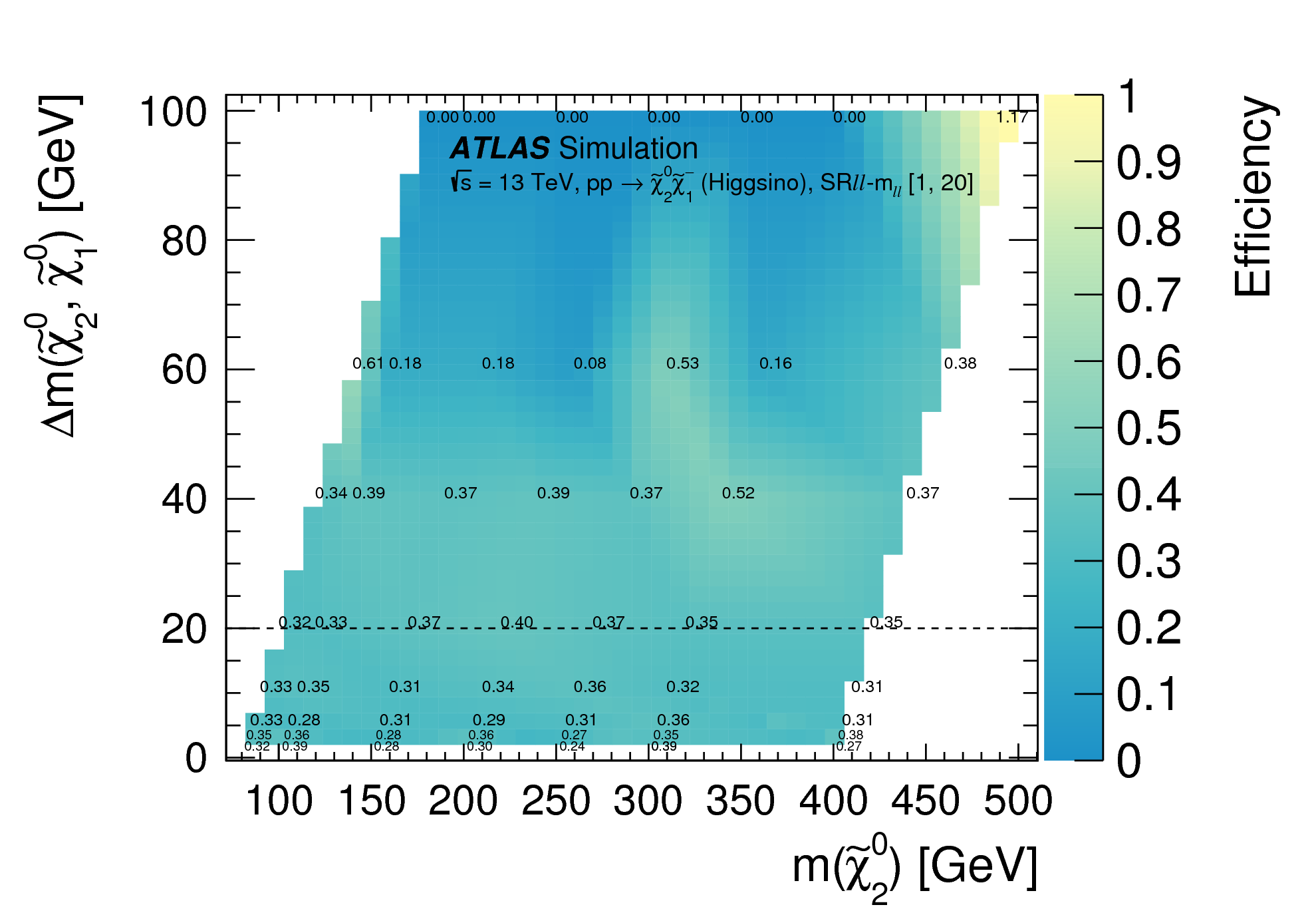
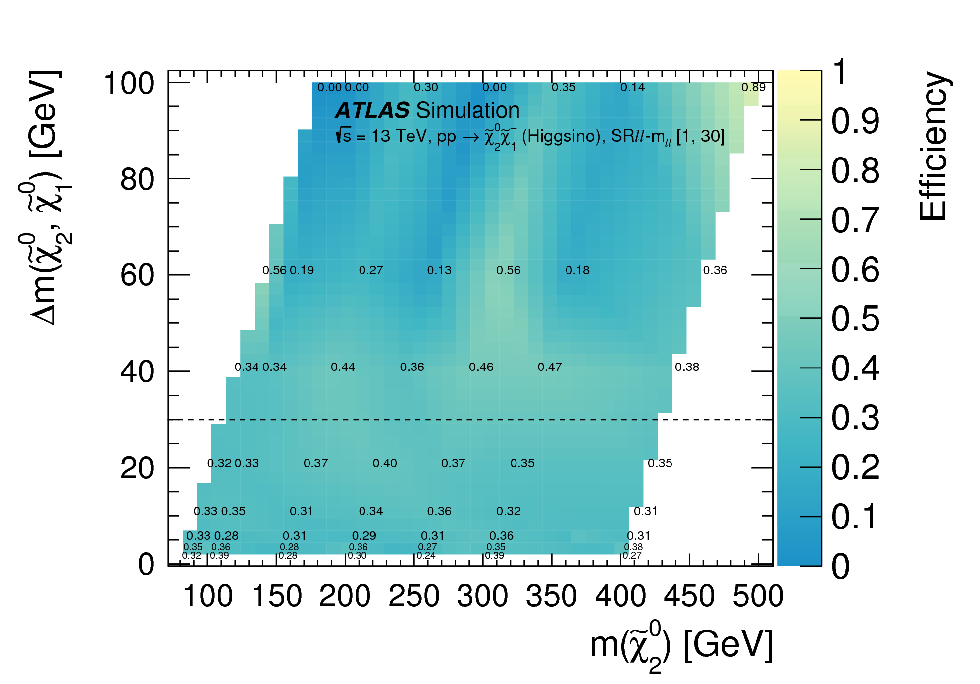
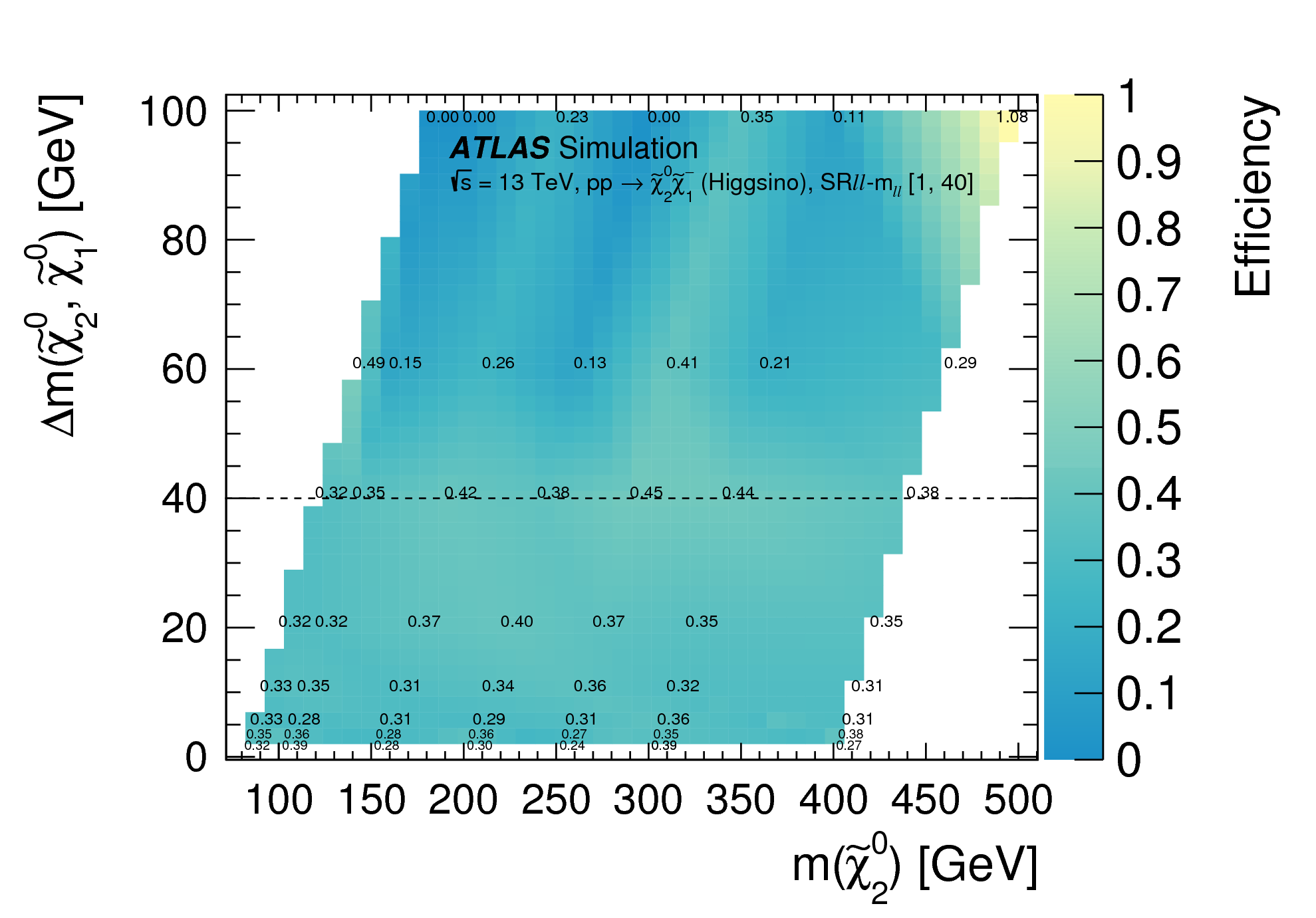
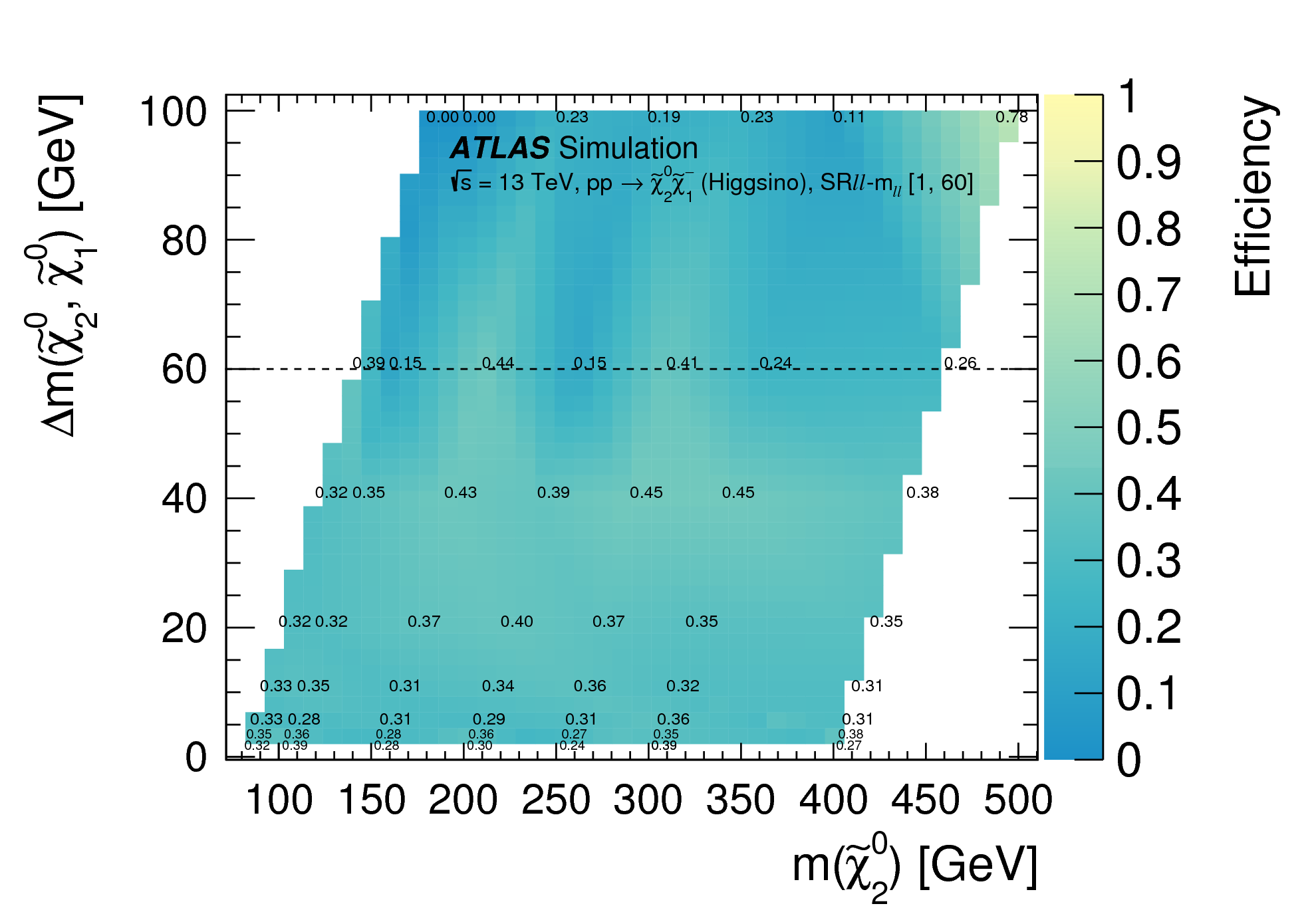
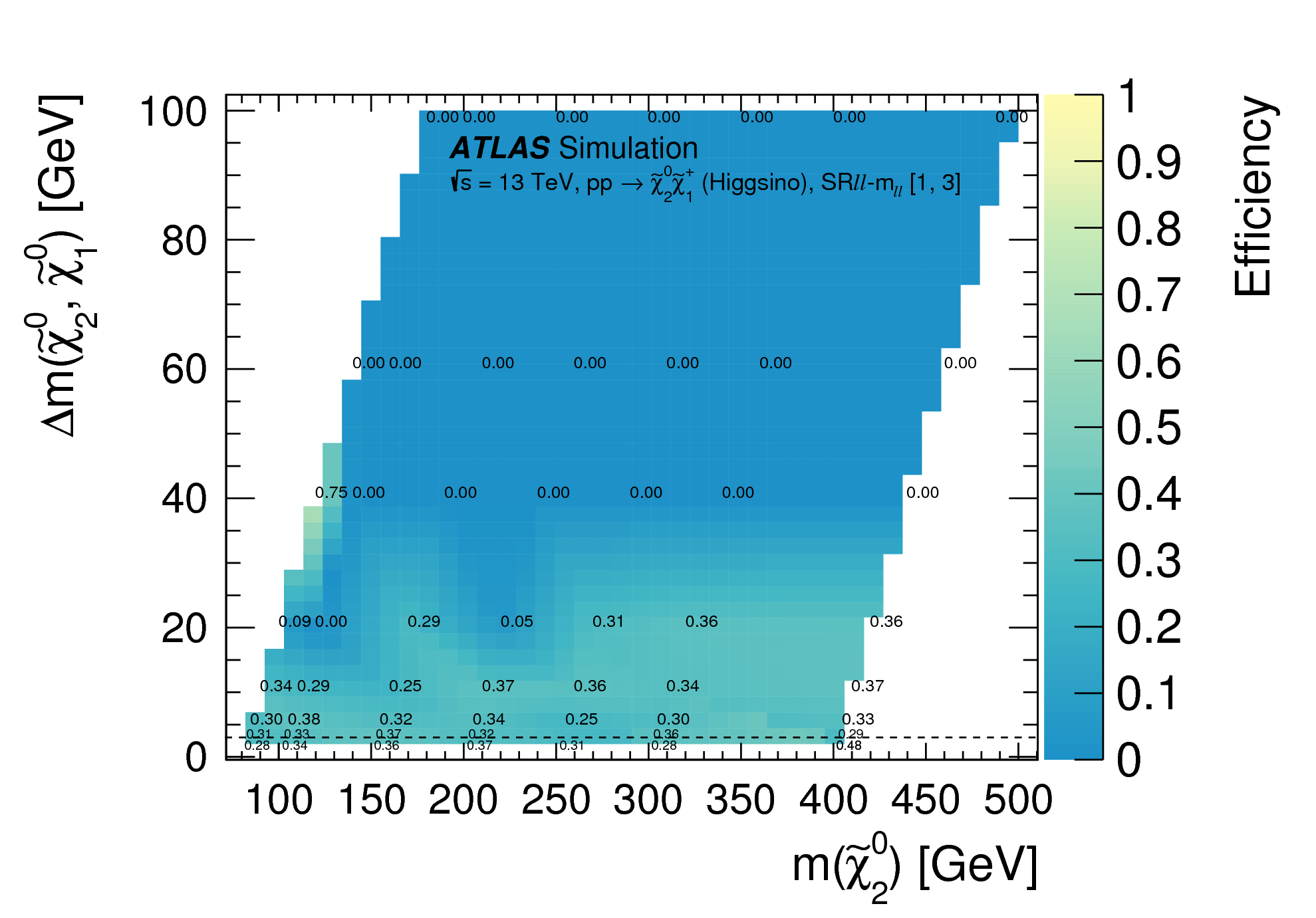
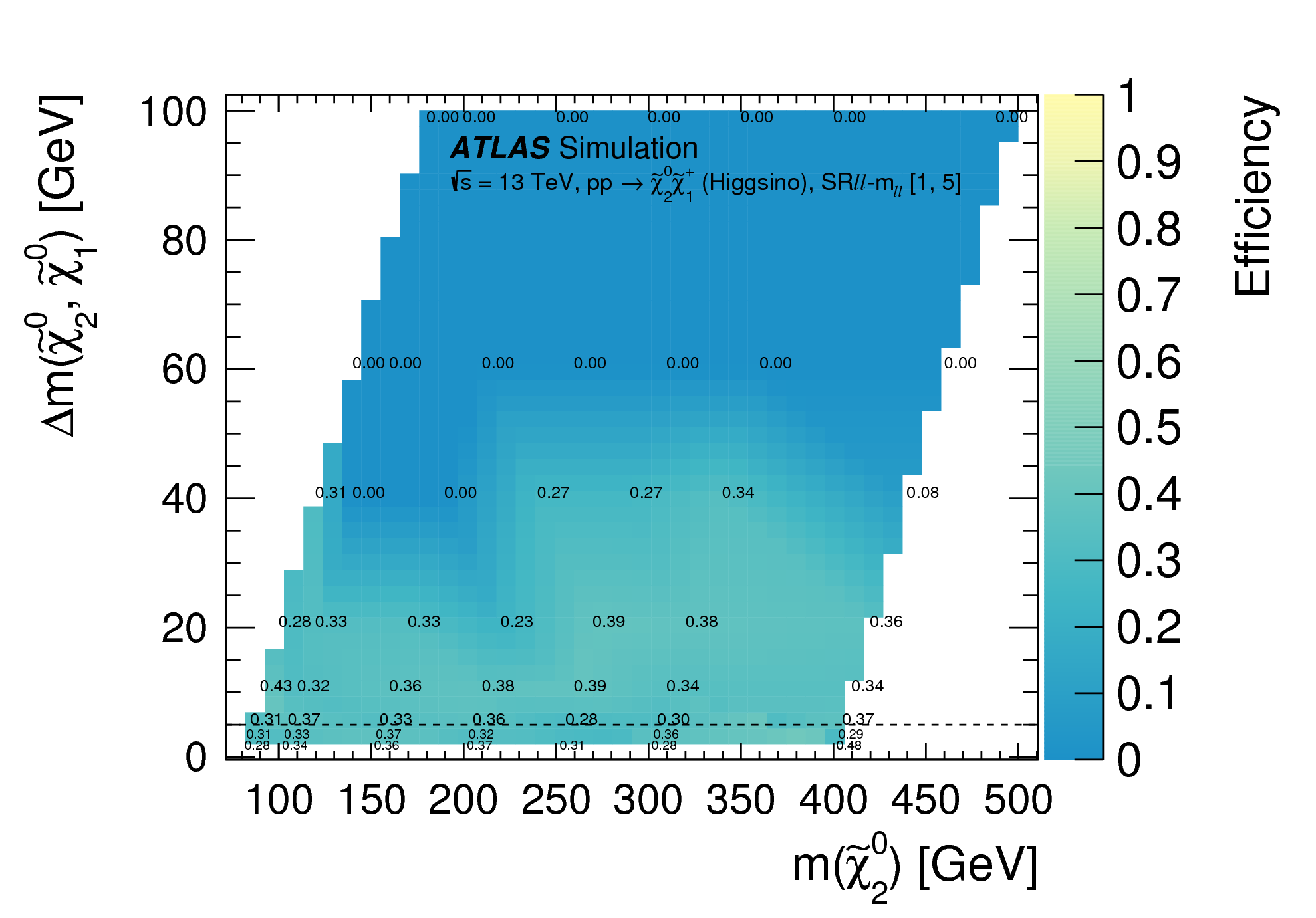
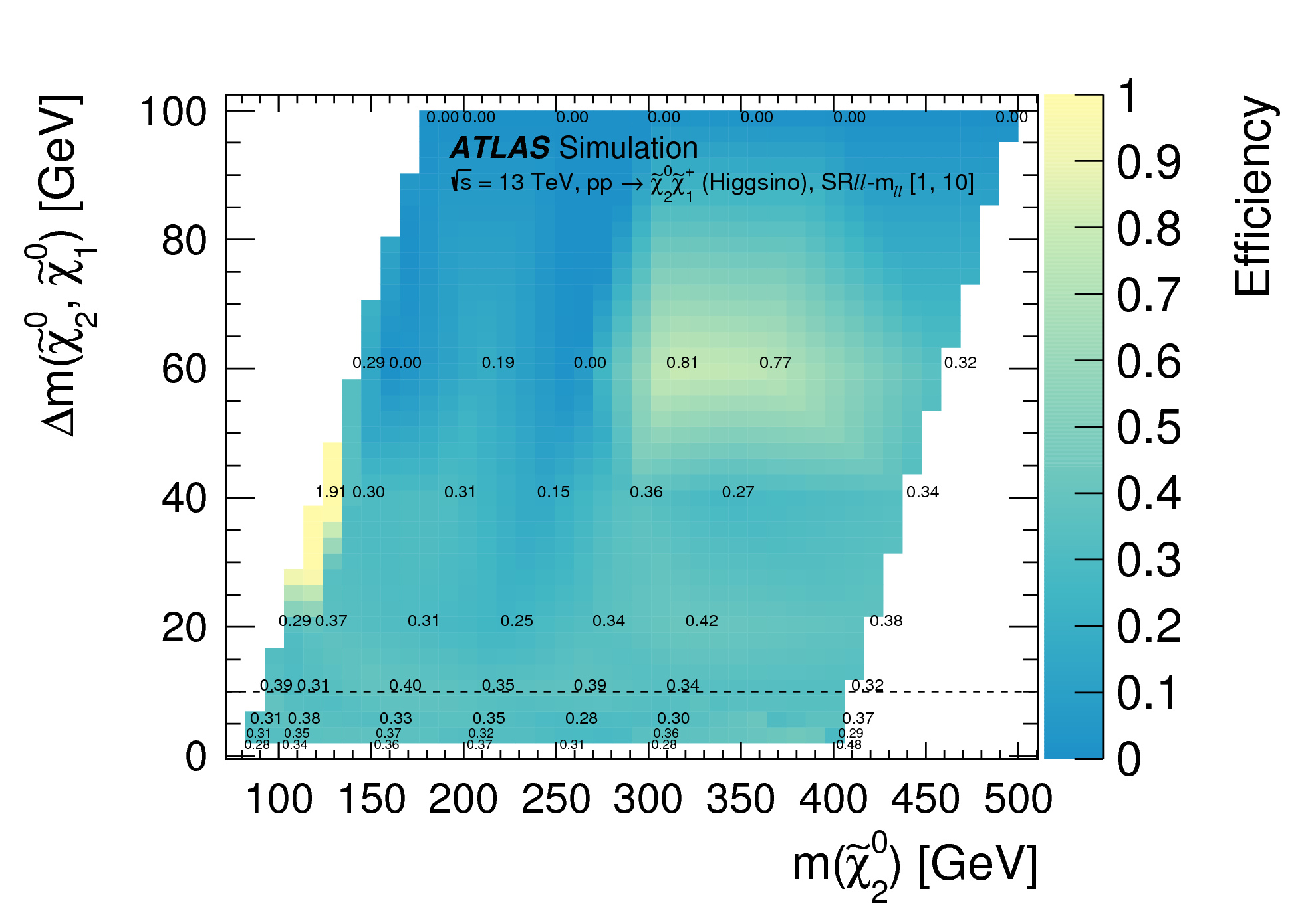
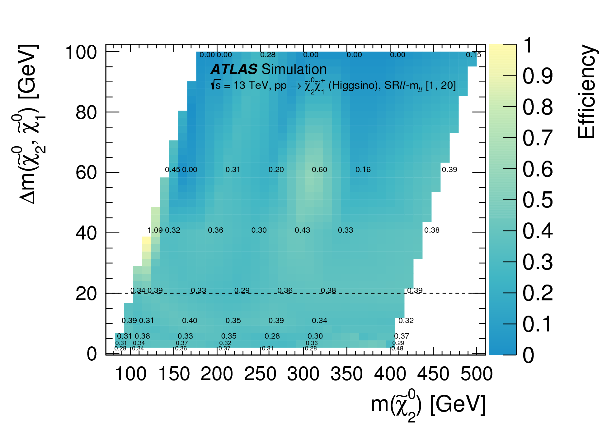
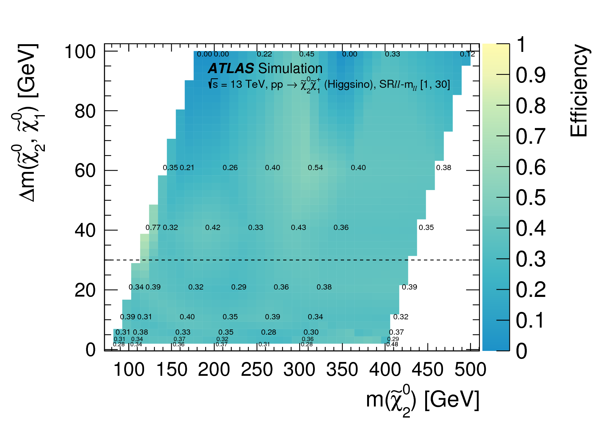
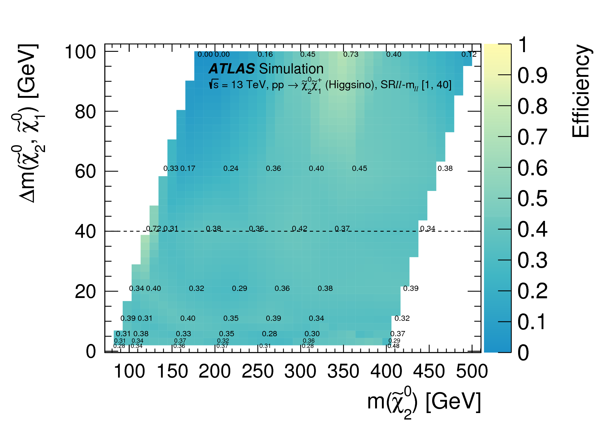
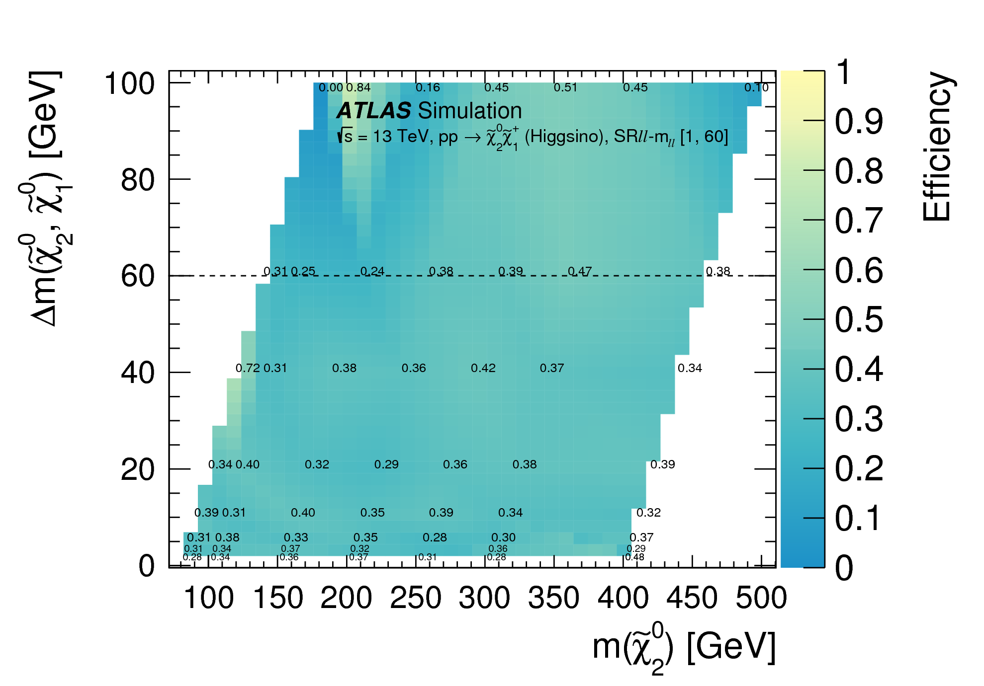
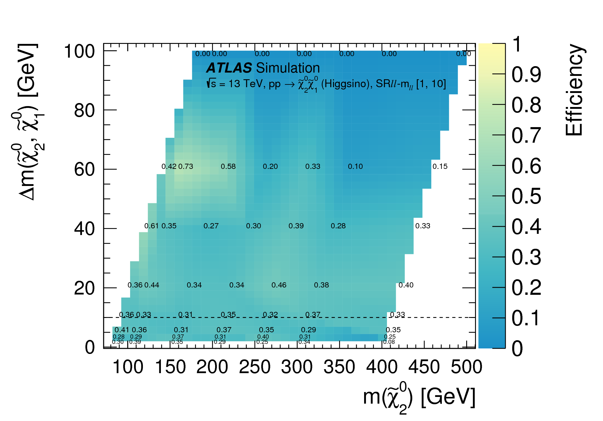
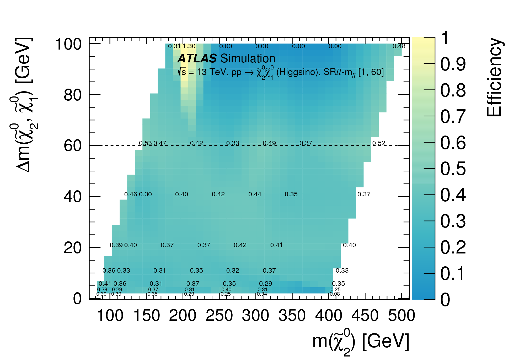
Figure 06a: Efficiencies for the Higgsino χ̃₂⁰χ̃₁⁺ production process in the inclusive SRℓℓ-m_ℓℓ regions. Efficiencies are computed as the ``acceptance times efficiency" divided by the acceptance. The black line indicates the maximum allowed value of Δ m or m_T2 for the inclusive signal region under study. png (120kB) pdf (33kB)
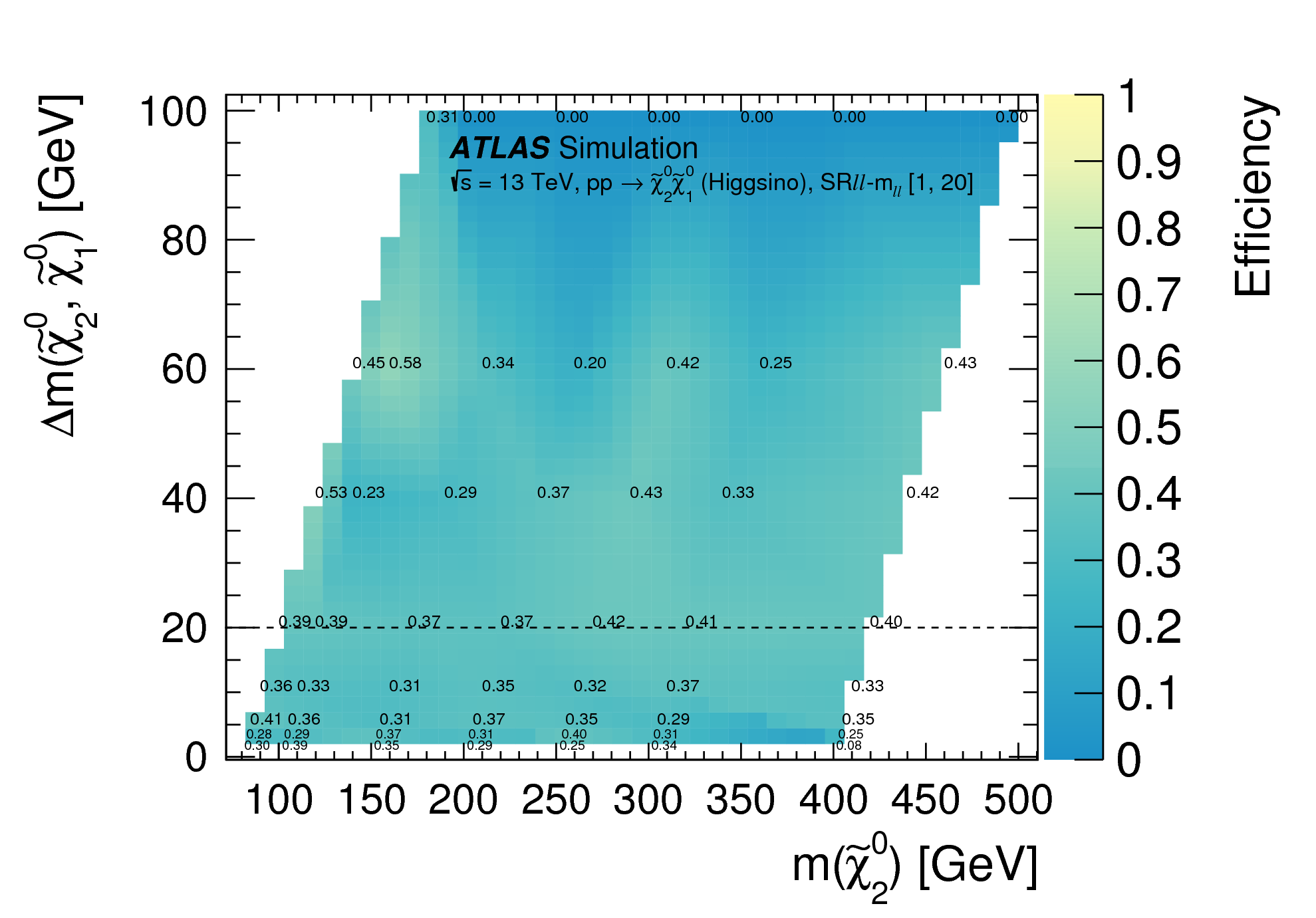
Figure 06b: Efficiencies for the Higgsino χ̃₂⁰χ̃₁⁺ production process in the inclusive SRℓℓ-m_ℓℓ regions. Efficiencies are computed as the ``acceptance times efficiency" divided by the acceptance. The black line indicates the maximum allowed value of Δ m or m_T2 for the inclusive signal region under study. png (125kB) pdf (33kB)
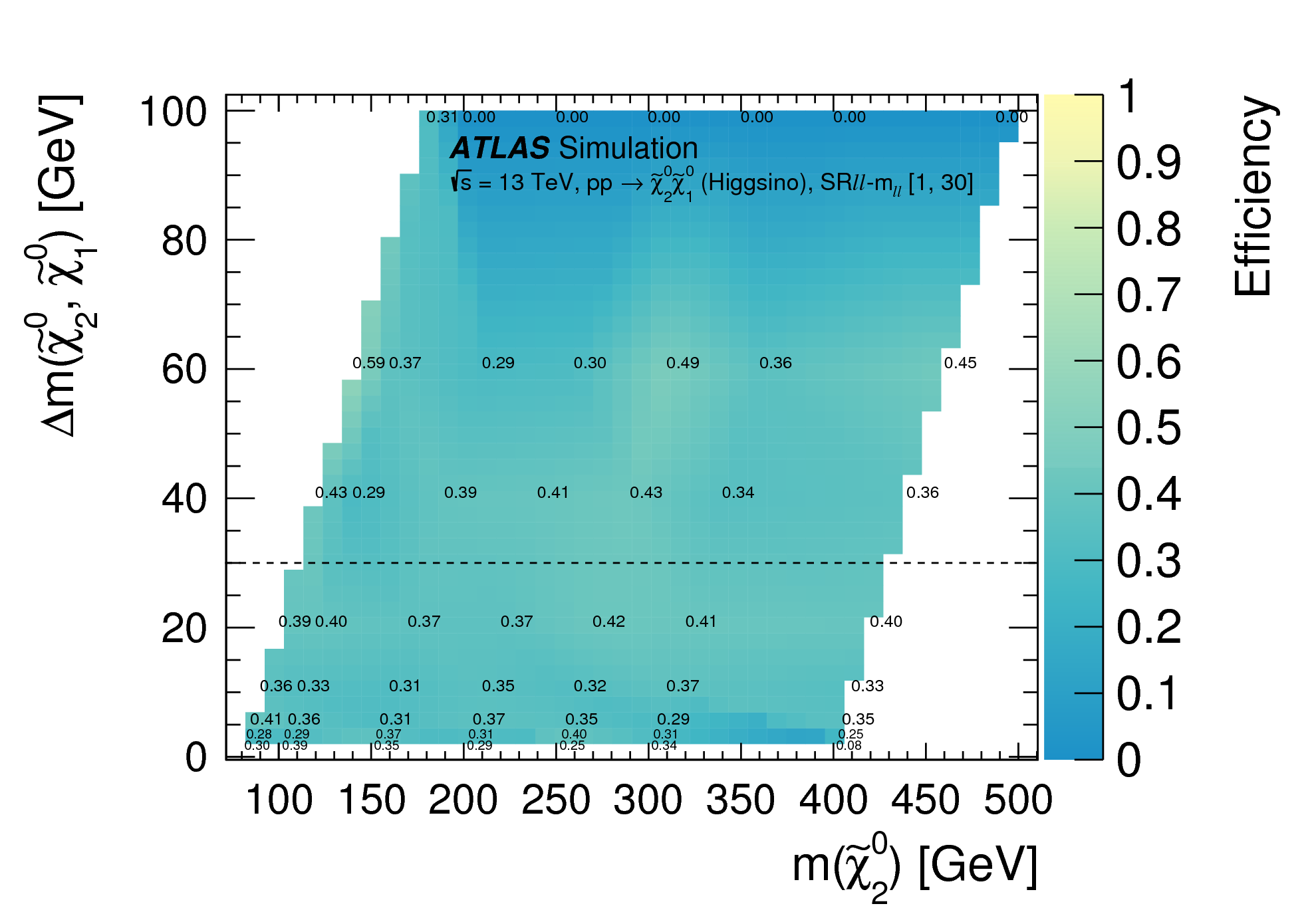
Figure 06c: Efficiencies for the Higgsino χ̃₂⁰χ̃₁⁺ production process in the inclusive SRℓℓ-m_ℓℓ regions. Efficiencies are computed as the ``acceptance times efficiency" divided by the acceptance. The black line indicates the maximum allowed value of Δ m or m_T2 for the inclusive signal region under study. png (139kB) pdf (37kB)
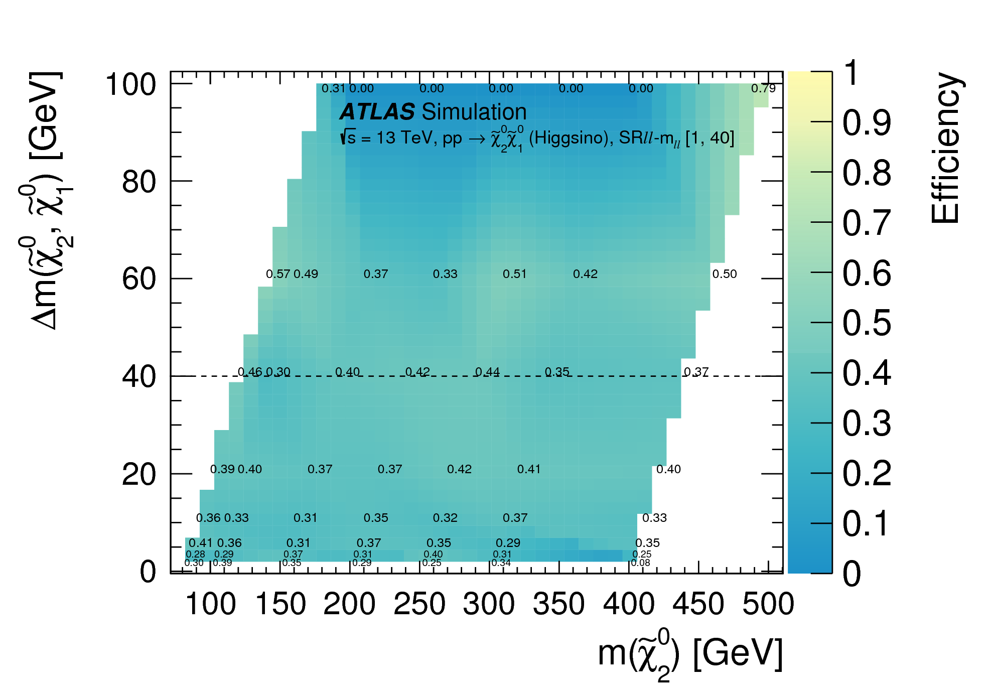
Figure 06d: Efficiencies for the Higgsino χ̃₂⁰χ̃₁⁺ production process in the inclusive SRℓℓ-m_ℓℓ regions. Efficiencies are computed as the ``acceptance times efficiency" divided by the acceptance. The black line indicates the maximum allowed value of Δ m or m_T2 for the inclusive signal region under study. png (145kB) pdf (35kB)
Figure 06e: Efficiencies for the Higgsino χ̃₂⁰χ̃₁⁺ production process in the inclusive SRℓℓ-m_ℓℓ regions. Efficiencies are computed as the ``acceptance times efficiency" divided by the acceptance. The black line indicates the maximum allowed value of Δ m or m_T2 for the inclusive signal region under study. png (146kB) pdf (35kB)
Figure 06f: Efficiencies for the Higgsino χ̃₂⁰χ̃₁⁺ production process in the inclusive SRℓℓ-m_ℓℓ regions. Efficiencies are computed as the ``acceptance times efficiency" divided by the acceptance. The black line indicates the maximum allowed value of Δ m or m_T2 for the inclusive signal region under study. png (146kB) pdf (36kB)
Figure 06g: Efficiencies for the Higgsino χ̃₂⁰χ̃₁⁺ production process in the inclusive SRℓℓ-m_ℓℓ regions. Efficiencies are computed as the ``acceptance times efficiency" divided by the acceptance. The black line indicates the maximum allowed value of Δ m or m_T2 for the inclusive signal region under study. png (146kB) pdf (36kB)
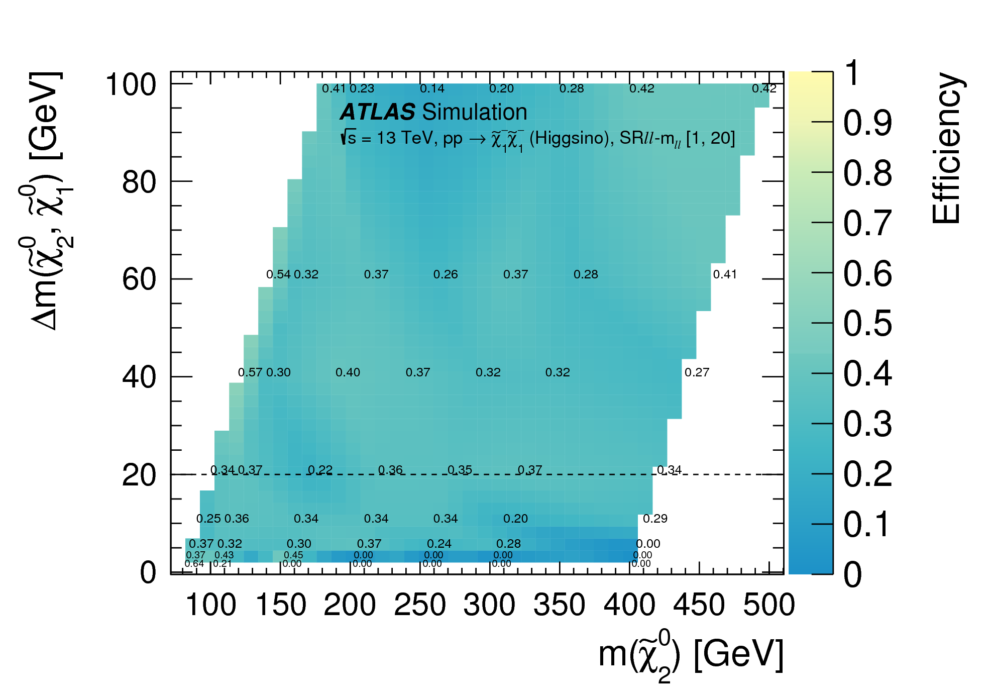
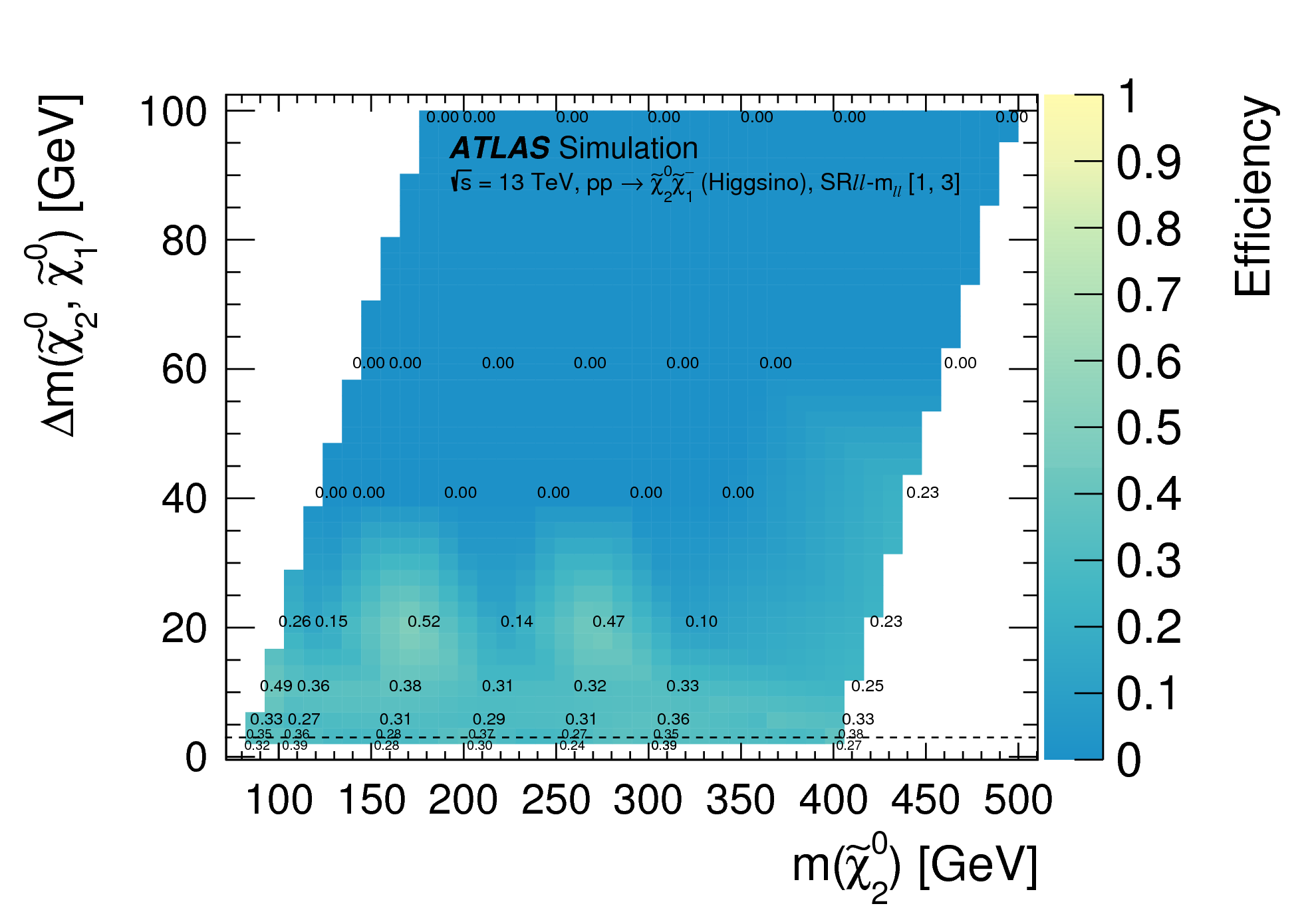
Figure 07a: Efficiencies for the Higgsino χ̃₂⁰χ̃₁^- production process in the inclusive SRℓℓ-m_ℓℓ regions. Efficiencies are computed as the ``acceptance times efficiency" divided by the acceptance. The black line indicates the maximum allowed value of Δ m or m_T2 for the inclusive signal region under study. png (120kB) pdf (33kB)
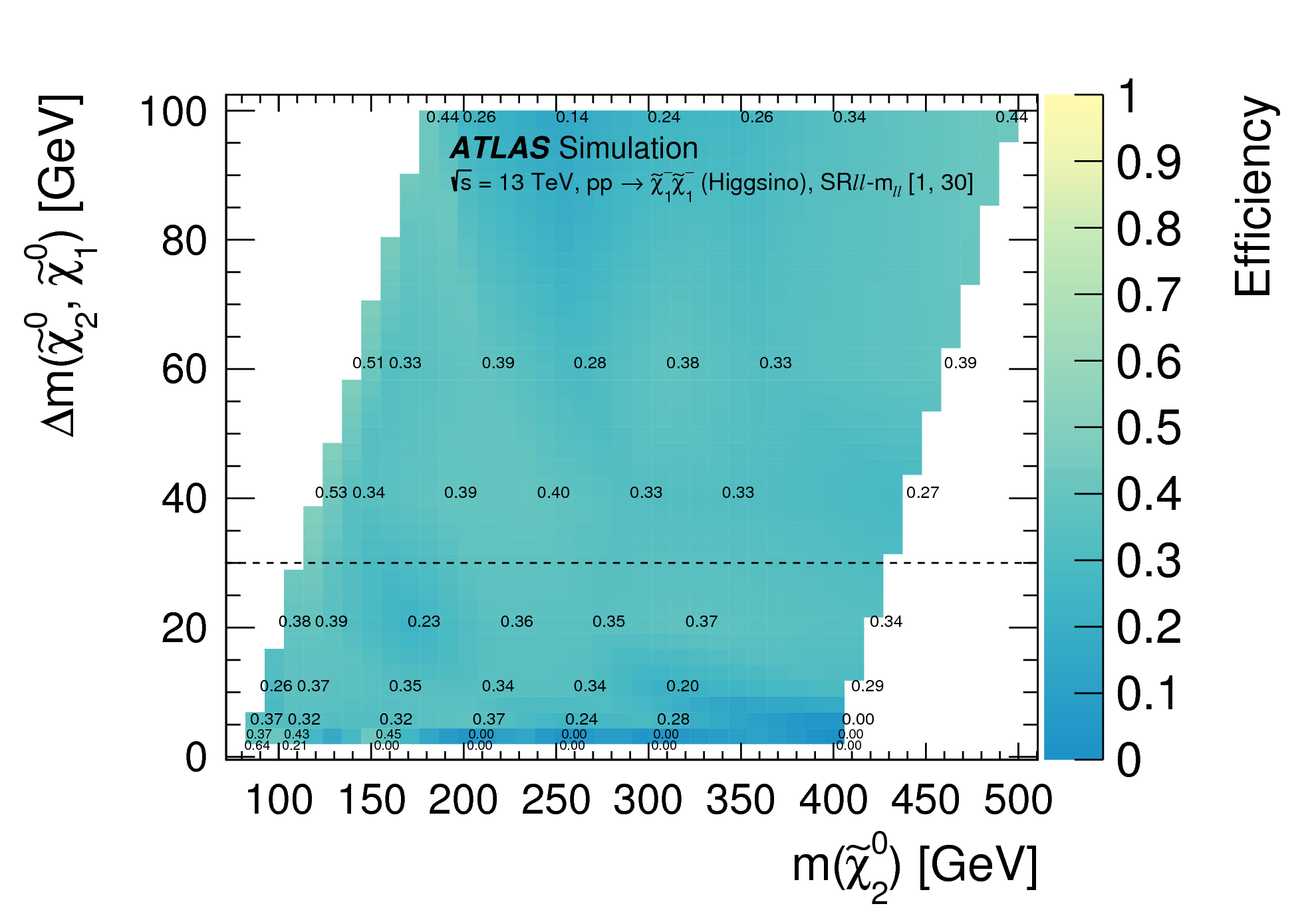
Figure 07b: Efficiencies for the Higgsino χ̃₂⁰χ̃₁^- production process in the inclusive SRℓℓ-m_ℓℓ regions. Efficiencies are computed as the ``acceptance times efficiency" divided by the acceptance. The black line indicates the maximum allowed value of Δ m or m_T2 for the inclusive signal region under study. png (126kB) pdf (34kB)
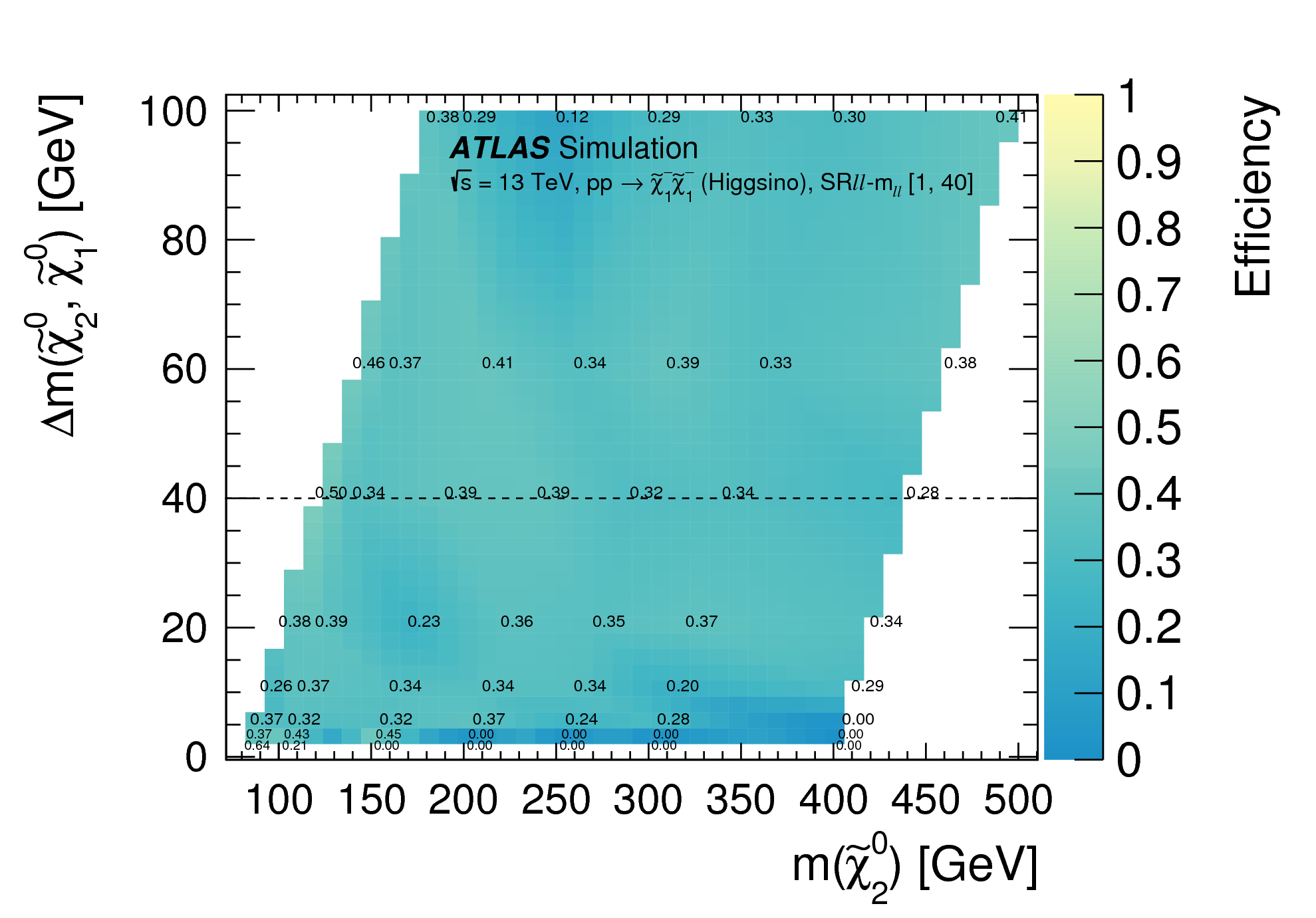
Figure 07c: Efficiencies for the Higgsino χ̃₂⁰χ̃₁^- production process in the inclusive SRℓℓ-m_ℓℓ regions. Efficiencies are computed as the ``acceptance times efficiency" divided by the acceptance. The black line indicates the maximum allowed value of Δ m or m_T2 for the inclusive signal region under study. png (138kB) pdf (36kB)
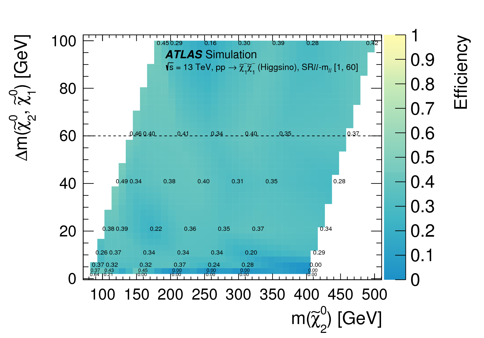
Figure 07d: Efficiencies for the Higgsino χ̃₂⁰χ̃₁^- production process in the inclusive SRℓℓ-m_ℓℓ regions. Efficiencies are computed as the ``acceptance times efficiency" divided by the acceptance. The black line indicates the maximum allowed value of Δ m or m_T2 for the inclusive signal region under study. png (140kB) pdf (36kB)
Figure 07e: Efficiencies for the Higgsino χ̃₂⁰χ̃₁^- production process in the inclusive SRℓℓ-m_ℓℓ regions. Efficiencies are computed as the ``acceptance times efficiency" divided by the acceptance. The black line indicates the maximum allowed value of Δ m or m_T2 for the inclusive signal region under study. png (145kB) pdf (36kB)
Figure 07f: Efficiencies for the Higgsino χ̃₂⁰χ̃₁^- production process in the inclusive SRℓℓ-m_ℓℓ regions. Efficiencies are computed as the ``acceptance times efficiency" divided by the acceptance. The black line indicates the maximum allowed value of Δ m or m_T2 for the inclusive signal region under study. png (143kB) pdf (36kB)
Figure 07g: Efficiencies for the Higgsino χ̃₂⁰χ̃₁^- production process in the inclusive SRℓℓ-m_ℓℓ regions. Efficiencies are computed as the ``acceptance times efficiency" divided by the acceptance. The black line indicates the maximum allowed value of Δ m or m_T2 for the inclusive signal region under study. png (144kB) pdf (35kB)
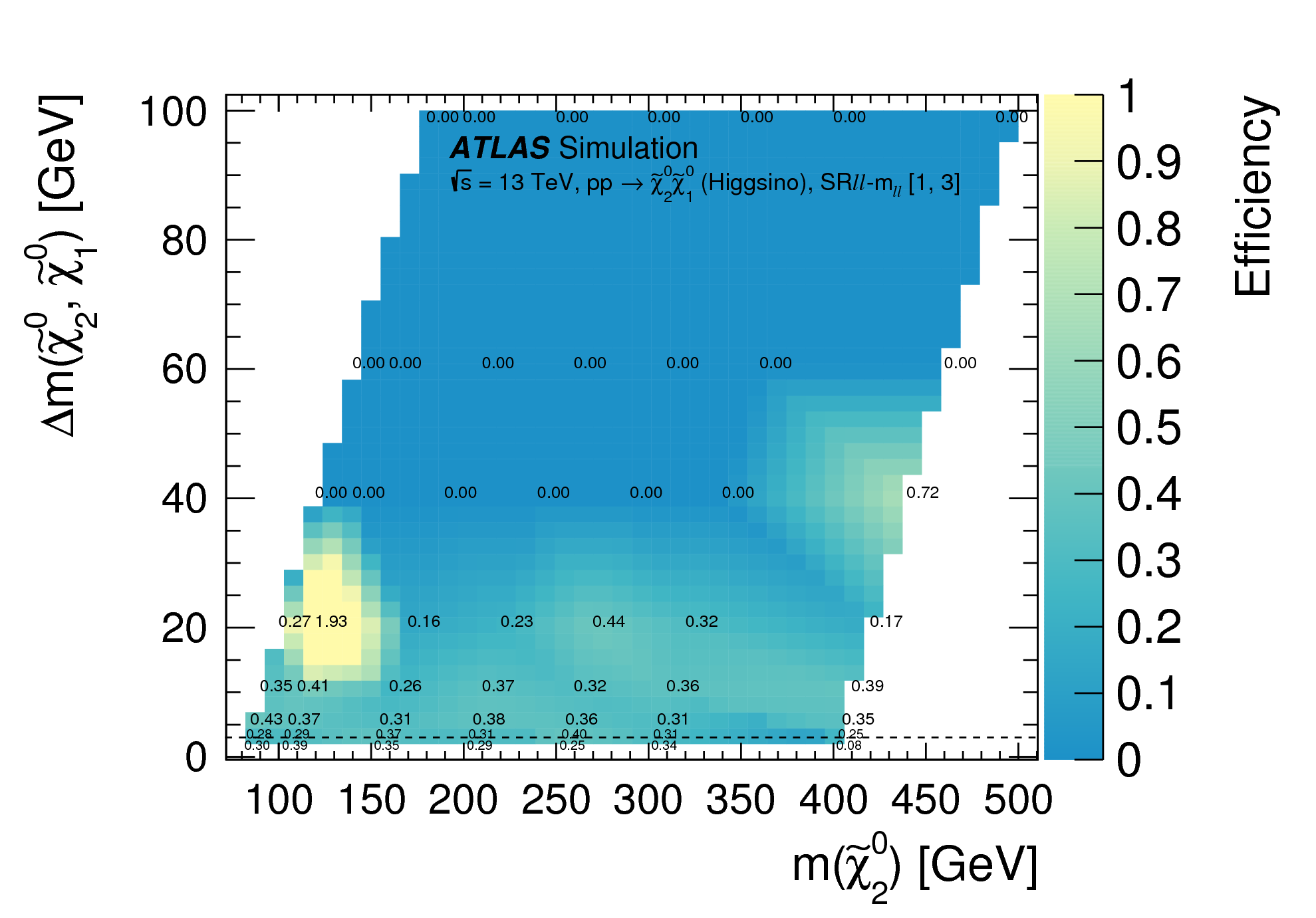
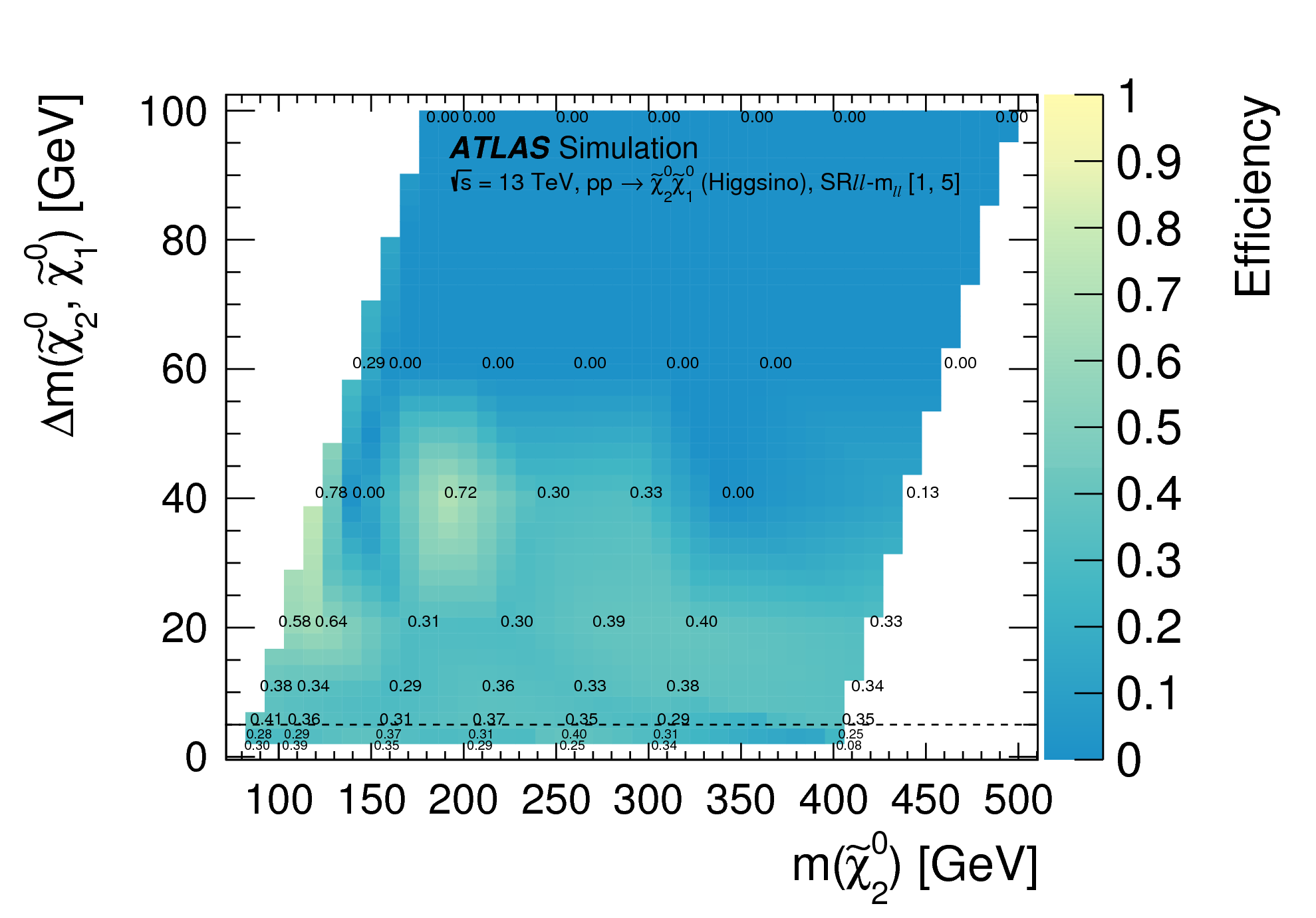
Figure 08a: Efficiencies for the Higgsino χ̃₂⁰χ̃₁⁰ production process in the inclusive SRℓℓ-m_ℓℓ regions. Efficiencies are computed as the ``acceptance times efficiency" divided by the acceptance. The black line indicates the maximum allowed value of Δ m or m_T2 for the inclusive signal region under study. png (121kB) pdf (34kB)
Figure 08b: Efficiencies for the Higgsino χ̃₂⁰χ̃₁⁰ production process in the inclusive SRℓℓ-m_ℓℓ regions. Efficiencies are computed as the ``acceptance times efficiency" divided by the acceptance. The black line indicates the maximum allowed value of Δ m or m_T2 for the inclusive signal region under study. png (128kB) pdf (35kB)
Figure 08c: Efficiencies for the Higgsino χ̃₂⁰χ̃₁⁰ production process in the inclusive SRℓℓ-m_ℓℓ regions. Efficiencies are computed as the ``acceptance times efficiency" divided by the acceptance. The black line indicates the maximum allowed value of Δ m or m_T2 for the inclusive signal region under study. png (138kB) pdf (36kB)
Figure 08d: Efficiencies for the Higgsino χ̃₂⁰χ̃₁⁰ production process in the inclusive SRℓℓ-m_ℓℓ regions. Efficiencies are computed as the ``acceptance times efficiency" divided by the acceptance. The black line indicates the maximum allowed value of Δ m or m_T2 for the inclusive signal region under study. png (139kB) pdf (35kB)
Figure 08e: Efficiencies for the Higgsino χ̃₂⁰χ̃₁⁰ production process in the inclusive SRℓℓ-m_ℓℓ regions. Efficiencies are computed as the ``acceptance times efficiency" divided by the acceptance. The black line indicates the maximum allowed value of Δ m or m_T2 for the inclusive signal region under study. png (138kB) pdf (35kB)
Figure 08f: Efficiencies for the Higgsino χ̃₂⁰χ̃₁⁰ production process in the inclusive SRℓℓ-m_ℓℓ regions. Efficiencies are computed as the ``acceptance times efficiency" divided by the acceptance. The black line indicates the maximum allowed value of Δ m or m_T2 for the inclusive signal region under study. png (138kB) pdf (35kB)
Figure 08g: Efficiencies for the Higgsino χ̃₂⁰χ̃₁⁰ production process in the inclusive SRℓℓ-m_ℓℓ regions. Efficiencies are computed as the ``acceptance times efficiency" divided by the acceptance. The black line indicates the maximum allowed value of Δ m or m_T2 for the inclusive signal region under study. png (141kB) pdf (35kB)
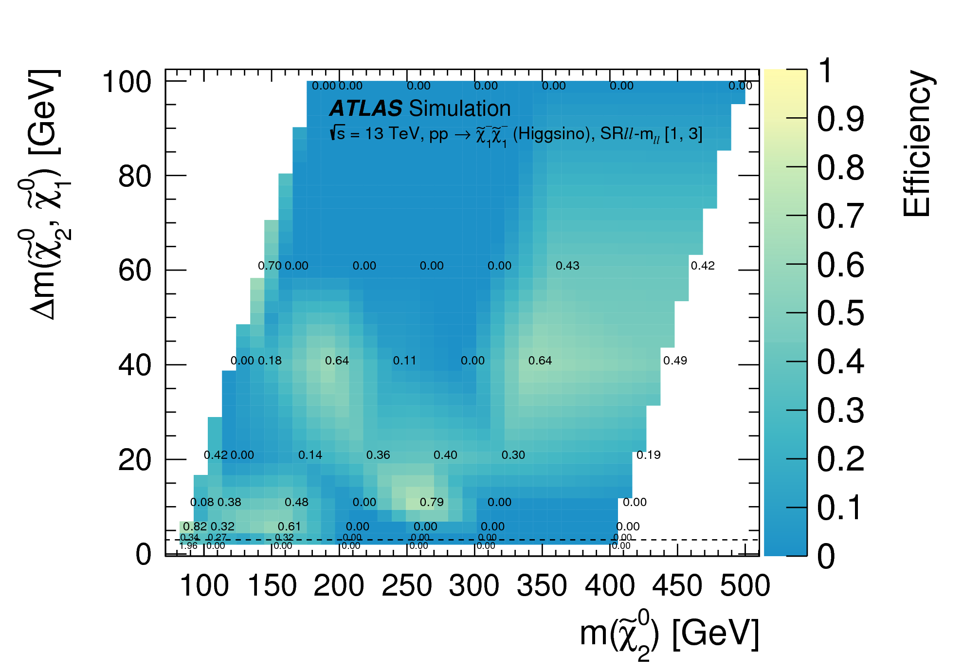
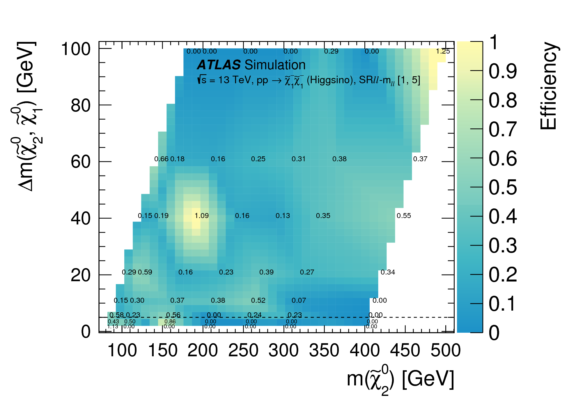
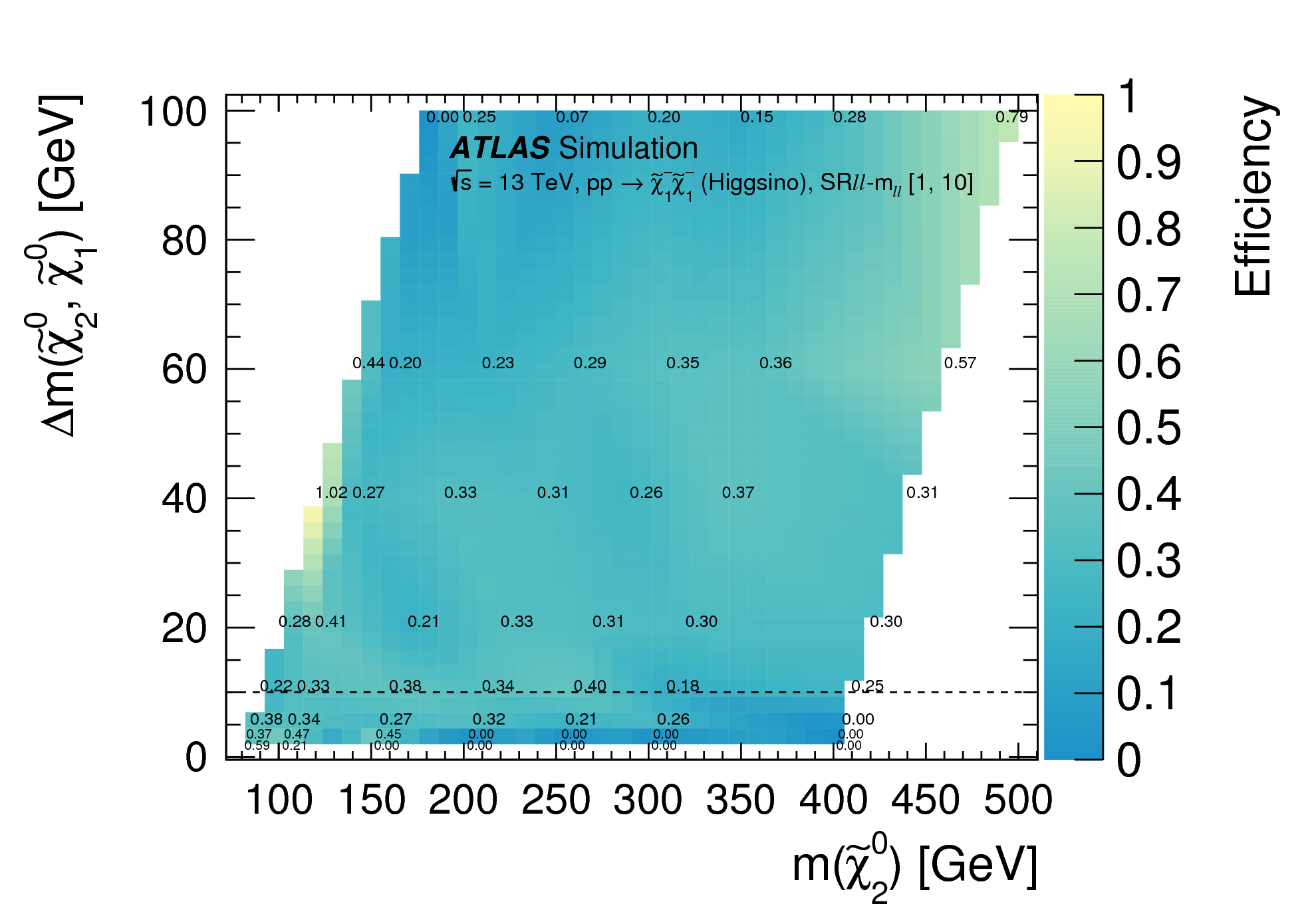
Figure 09a: Efficiencies for the Higgsino χ̃₁⁺χ̃₁^- production process in the inclusive SRℓℓ-m_ℓℓ regions. Efficiencies are computed as the ``acceptance times efficiency" divided by the acceptance. The black line indicates the maximum allowed value of Δ m or m_T2 for the inclusive signal region under study. png (128kB) pdf (36kB)
Figure 09b: Efficiencies for the Higgsino χ̃₁⁺χ̃₁^- production process in the inclusive SRℓℓ-m_ℓℓ regions. Efficiencies are computed as the ``acceptance times efficiency" divided by the acceptance. The black line indicates the maximum allowed value of Δ m or m_T2 for the inclusive signal region under study. png (142kB) pdf (38kB)
Figure 09c: Efficiencies for the Higgsino χ̃₁⁺χ̃₁^- production process in the inclusive SRℓℓ-m_ℓℓ regions. Efficiencies are computed as the ``acceptance times efficiency" divided by the acceptance. The black line indicates the maximum allowed value of Δ m or m_T2 for the inclusive signal region under study. png (141kB) pdf (36kB)
Figure 09d: Efficiencies for the Higgsino χ̃₁⁺χ̃₁^- production process in the inclusive SRℓℓ-m_ℓℓ regions. Efficiencies are computed as the ``acceptance times efficiency" divided by the acceptance. The black line indicates the maximum allowed value of Δ m or m_T2 for the inclusive signal region under study. png (141kB) pdf (35kB)
Figure 09e: Efficiencies for the Higgsino χ̃₁⁺χ̃₁^- production process in the inclusive SRℓℓ-m_ℓℓ regions. Efficiencies are computed as the ``acceptance times efficiency" divided by the acceptance. The black line indicates the maximum allowed value of Δ m or m_T2 for the inclusive signal region under study. png (142kB) pdf (35kB)
Figure 09f: Efficiencies for the Higgsino χ̃₁⁺χ̃₁^- production process in the inclusive SRℓℓ-m_ℓℓ regions. Efficiencies are computed as the ``acceptance times efficiency" divided by the acceptance. The black line indicates the maximum allowed value of Δ m or m_T2 for the inclusive signal region under study. png (141kB) pdf (35kB)
Figure 09g: Efficiencies for the Higgsino χ̃₁⁺χ̃₁^- production process in the inclusive SRℓℓ-m_ℓℓ regions. Efficiencies are computed as the ``acceptance times efficiency" divided by the acceptance. The black line indicates the maximum allowed value of Δ m or m_T2 for the inclusive signal region under study. png (142kB) pdf (35kB)
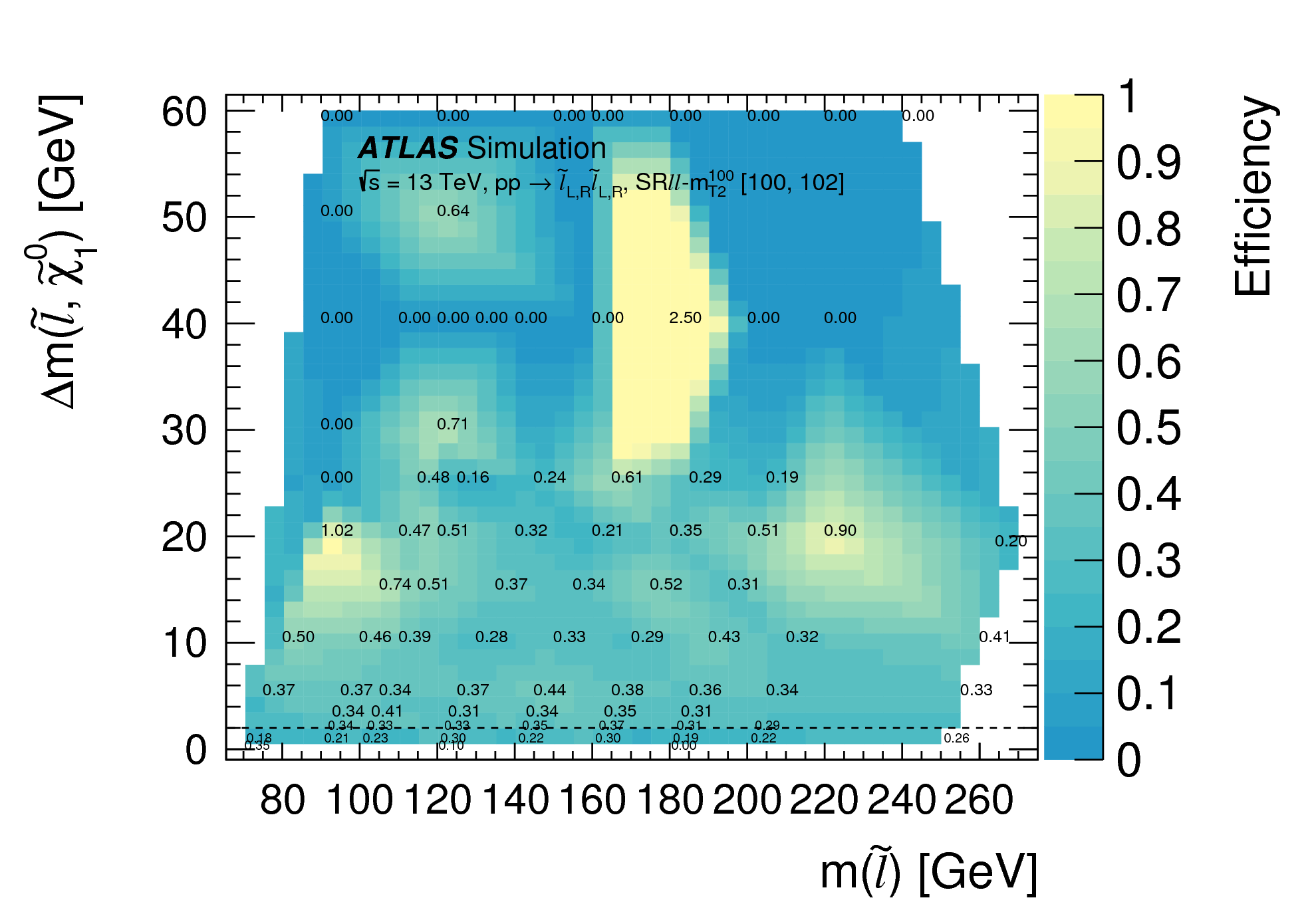
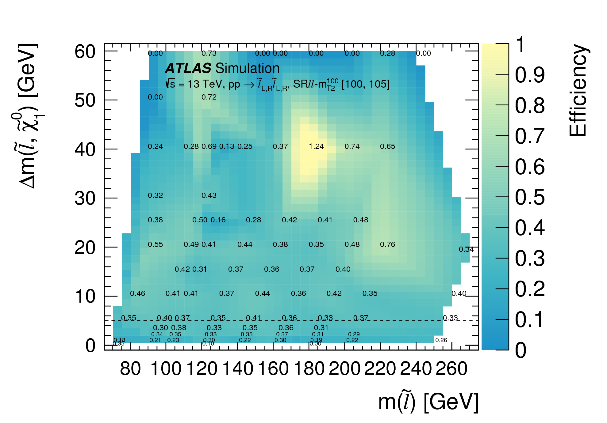
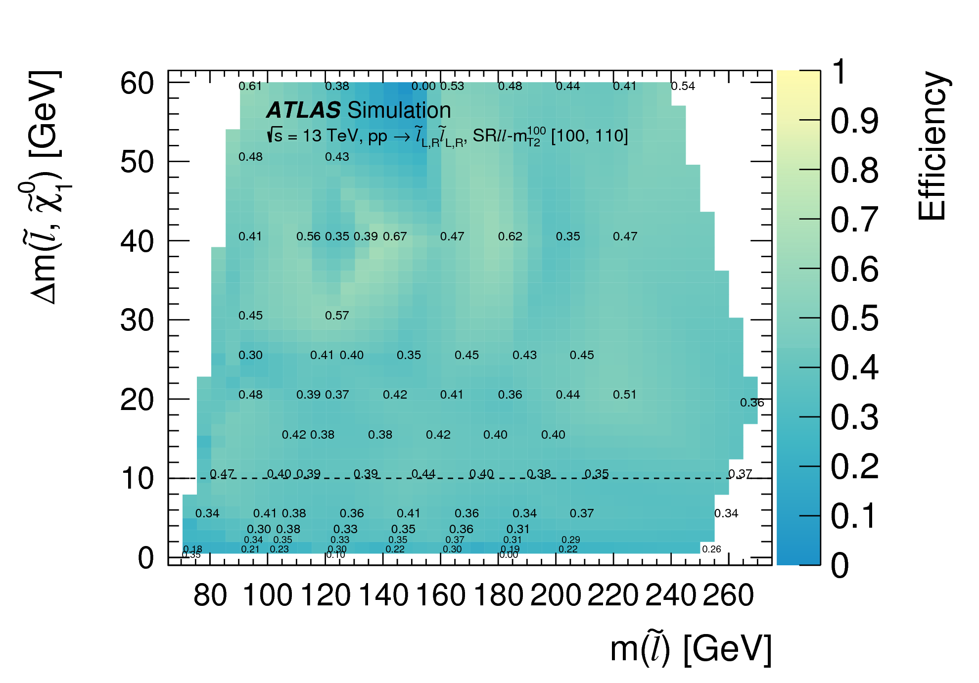
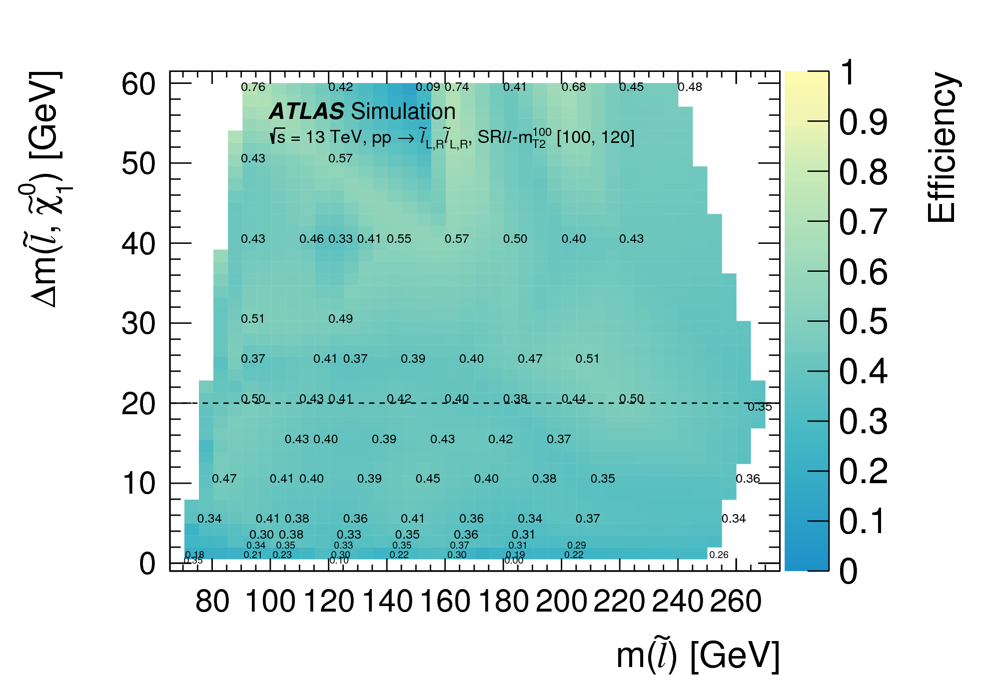
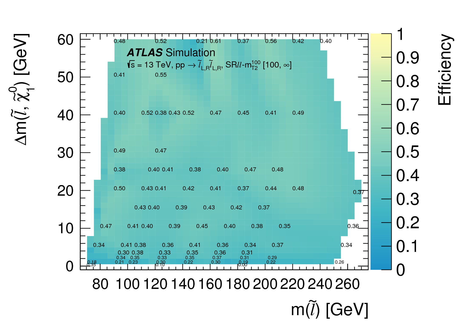
Figure 10a: Efficiencies for the ℓ̃ℓ̃ production in the inclusive SRℓℓ-m_T2¹⁰⁰ regions. Efficiencies are computed as the ``acceptance times efficiency" divided by the acceptance. The black line indicates the maximum allowed value of Δ m or m_T2 for the inclusive signal region under study. png (145kB) pdf (23kB)
Figure 10b: Efficiencies for the ℓ̃ℓ̃ production in the inclusive SRℓℓ-m_T2¹⁰⁰ regions. Efficiencies are computed as the ``acceptance times efficiency" divided by the acceptance. The black line indicates the maximum allowed value of Δ m or m_T2 for the inclusive signal region under study. png (172kB) pdf (40kB)
Figure 10c: Efficiencies for the ℓ̃ℓ̃ production in the inclusive SRℓℓ-m_T2¹⁰⁰ regions. Efficiencies are computed as the ``acceptance times efficiency" divided by the acceptance. The black line indicates the maximum allowed value of Δ m or m_T2 for the inclusive signal region under study. png (170kB) pdf (38kB)
Figure 10d: Efficiencies for the ℓ̃ℓ̃ production in the inclusive SRℓℓ-m_T2¹⁰⁰ regions. Efficiencies are computed as the ``acceptance times efficiency" divided by the acceptance. The black line indicates the maximum allowed value of Δ m or m_T2 for the inclusive signal region under study. png (169kB) pdf (37kB)
Figure 10e: Efficiencies for the ℓ̃ℓ̃ production in the inclusive SRℓℓ-m_T2¹⁰⁰ regions. Efficiencies are computed as the ``acceptance times efficiency" divided by the acceptance. The black line indicates the maximum allowed value of Δ m or m_T2 for the inclusive signal region under study. png (167kB) pdf (37kB)
Figure 10f: Efficiencies for the ℓ̃ℓ̃ production in the inclusive SRℓℓ-m_T2¹⁰⁰ regions. Efficiencies are computed as the ``acceptance times efficiency" divided by the acceptance. The black line indicates the maximum allowed value of Δ m or m_T2 for the inclusive signal region under study. png (164kB) pdf (37kB)
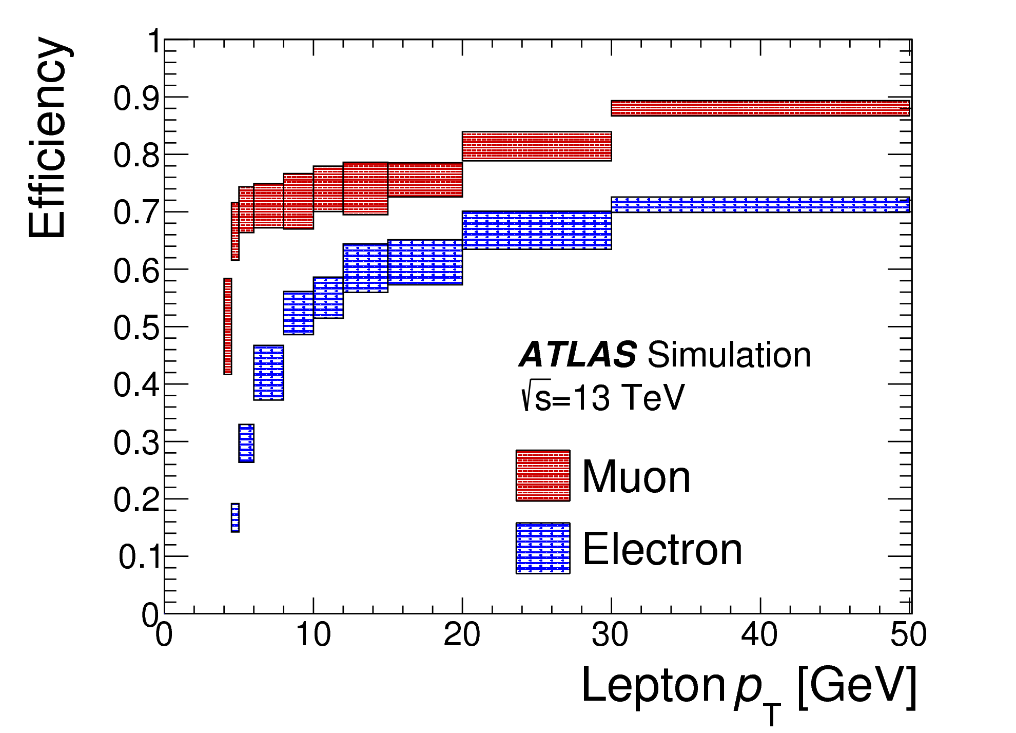
Figure 11: Signal lepton efficiencies for electrons and muons, averaged over all Higgsino and slepton samples. Efficiencies are shown for leptons within detector acceptance, and with lepton p_T within a factor of 3 of Δ m(ℓ,χ̃₁⁰) for slepton samples, or within a factor of 3 of Δ m(χ̃₂⁰,χ̃₁⁰)/2 for Higgsino samples. Uncertainty bands represent the range of efficiencies observed across all signal samples for the given p_T bin. The η-dependence is consistent with values reported in ATLAS combined performance papers. png (32kB) pdf (15kB)
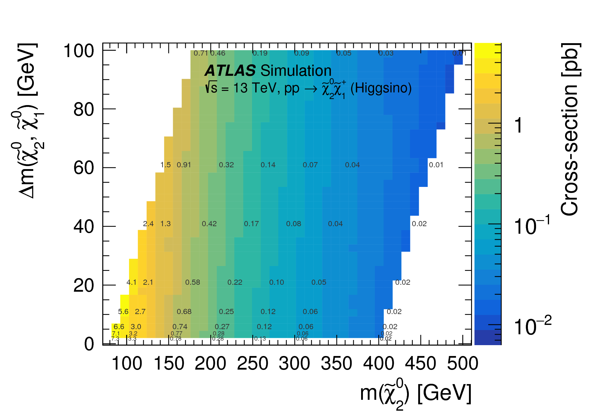
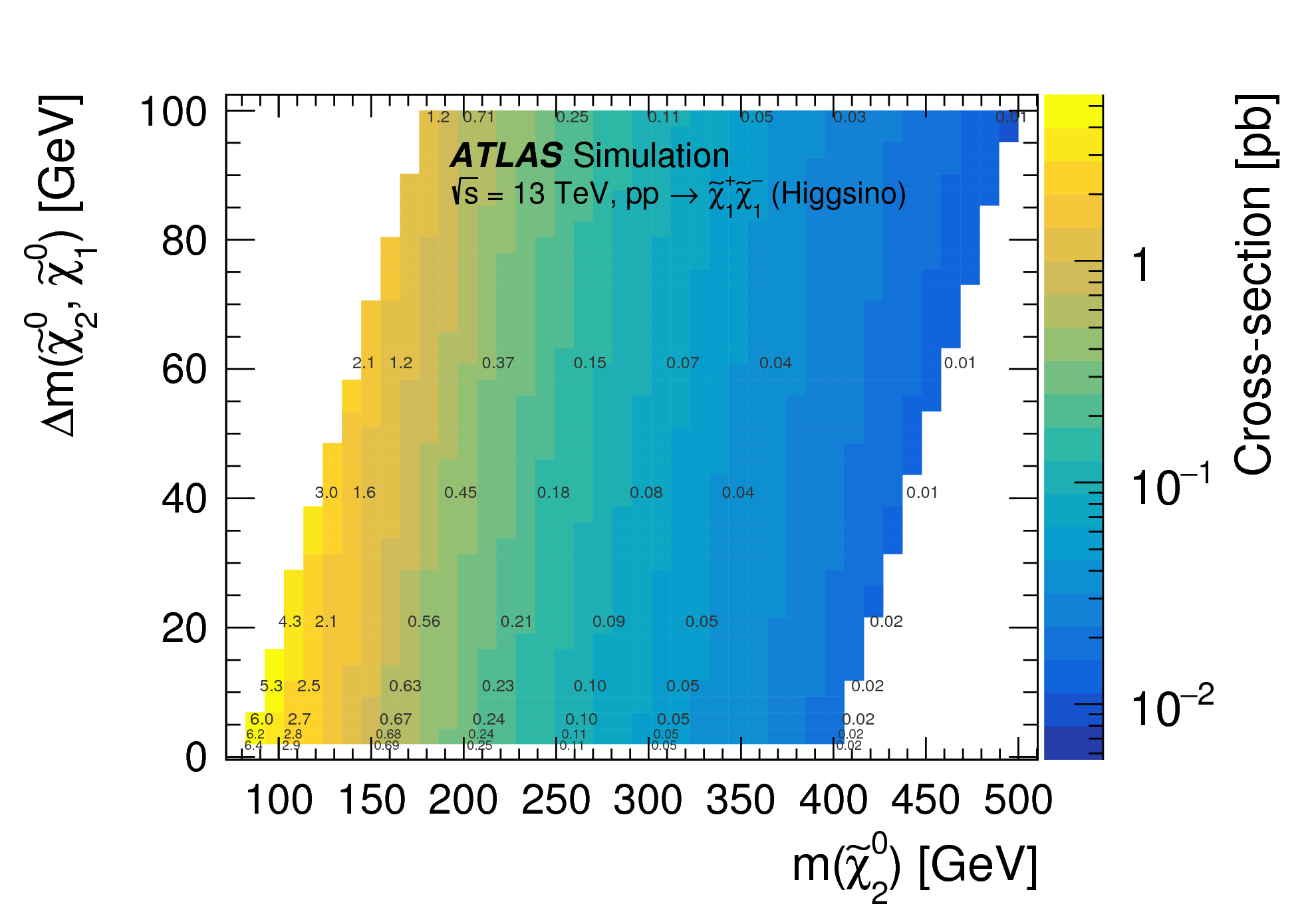
Figure 12a: Cross-sections of the Higgsino signal grid for each production process denoted in the caption. png (126kB) pdf (21kB)
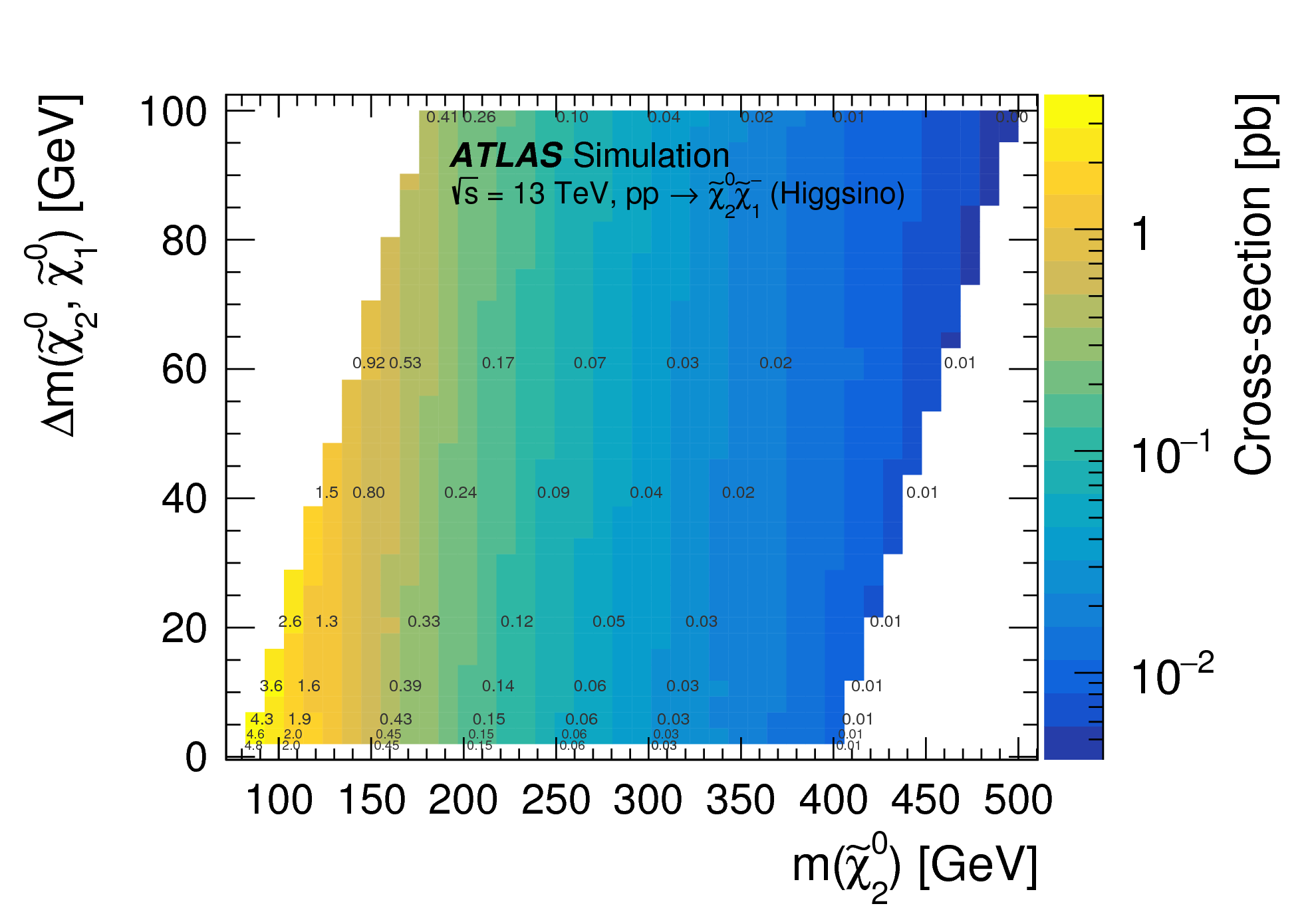
Figure 12b: Cross-sections of the Higgsino signal grid for each production process denoted in the caption. png (128kB) pdf (21kB)
Figure 12c: Cross-sections of the Higgsino signal grid for each production process denoted in the caption. png (127kB) pdf (21kB)
Figure 12d: Cross-sections of the Higgsino signal grid for each production process denoted in the caption. png (126kB) pdf (21kB)
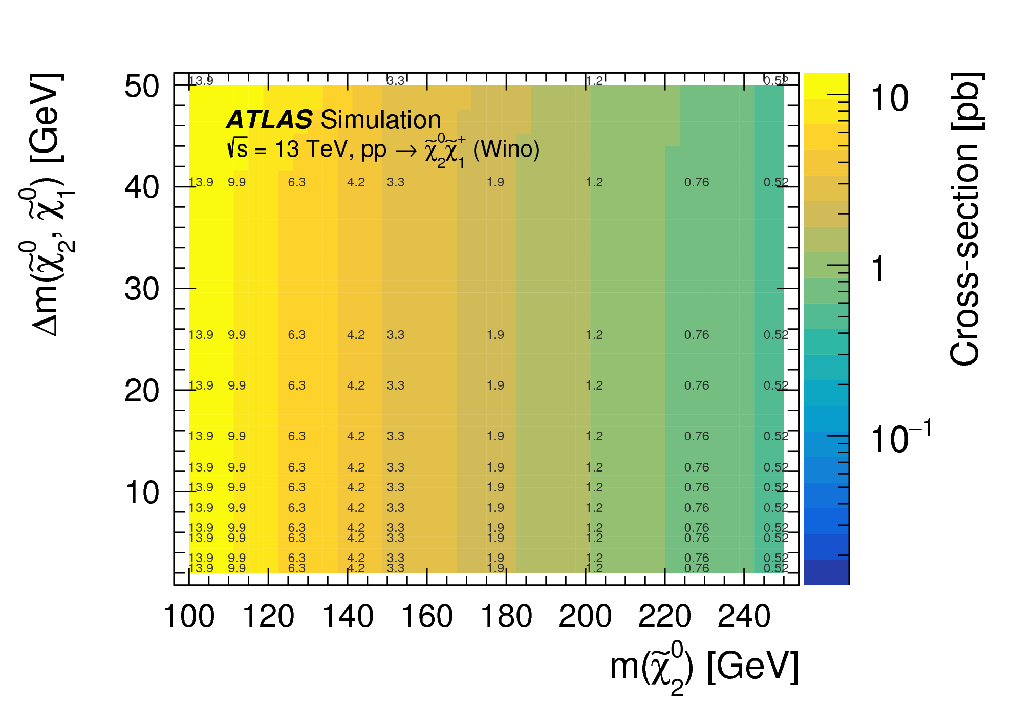
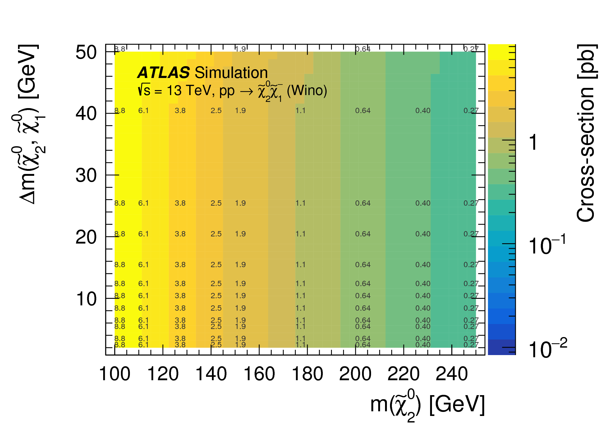
Figure 13a: Cross-sections of the wino--bino signal grid for each production process in the caption. png (158kB) pdf (22kB)
Figure 13b: Cross-sections of the wino--bino signal grid for each production process in the caption. png (150kB) pdf (22kB)
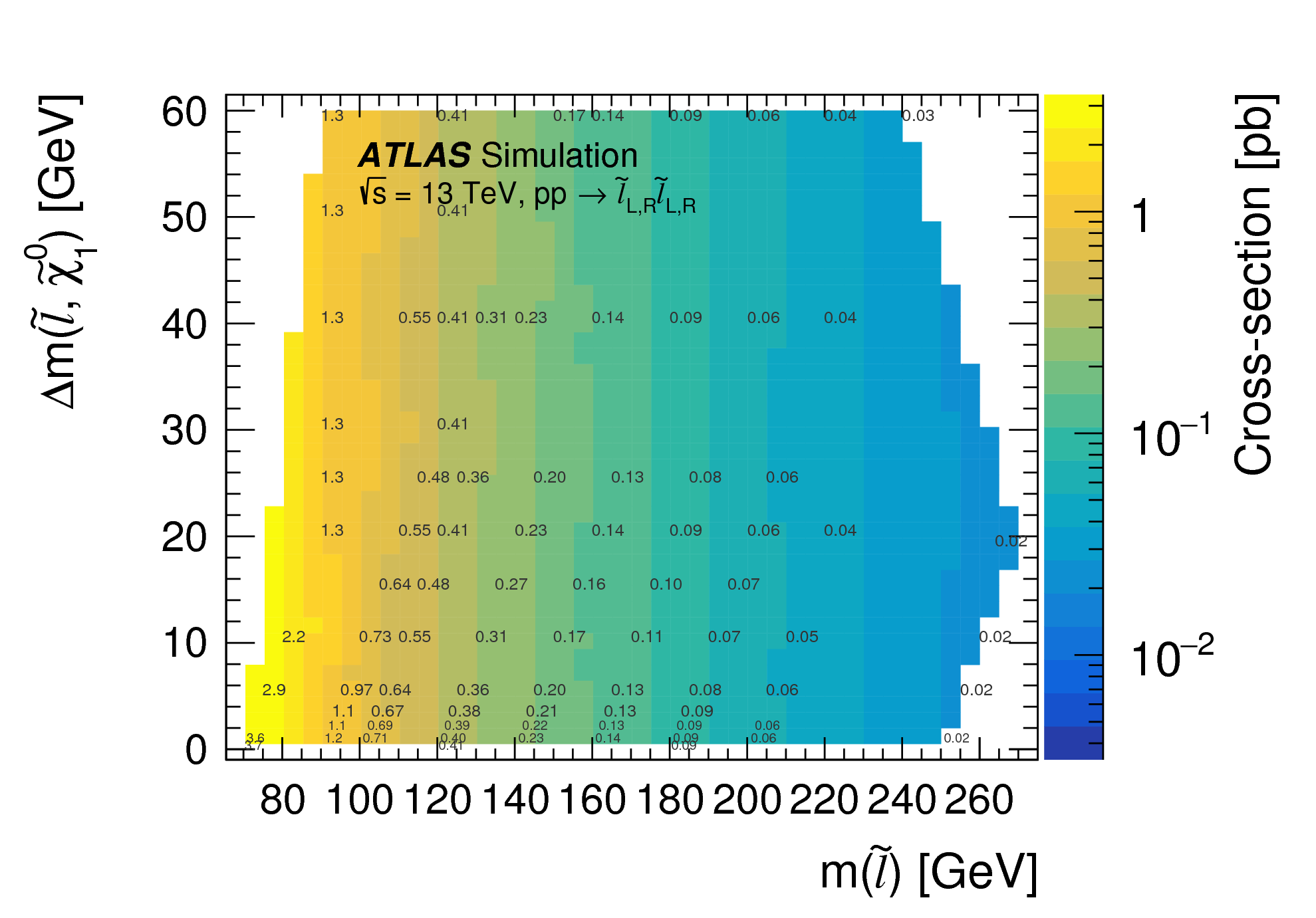
Figure 14: Total cross-sections of the slepton simplified model signal grid. Slepton refers to a the scalar partners of the left- and right-handed electrons and muons, which are assumed to be mass degenerate m(ẽ_L) = m(ẽ_R) = m(μ̃_L) = m(μ̃_R). png (145kB) pdf (22kB)
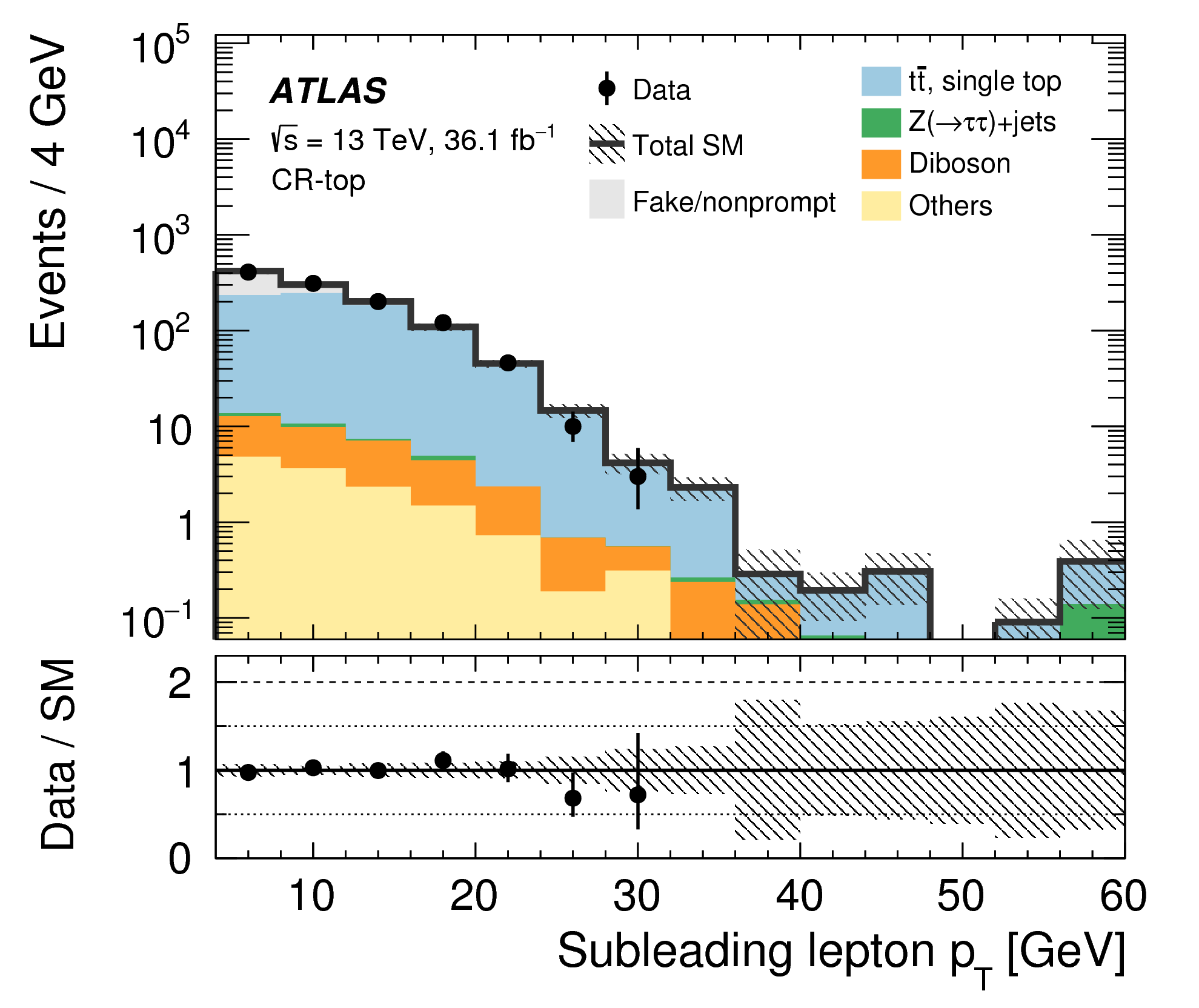
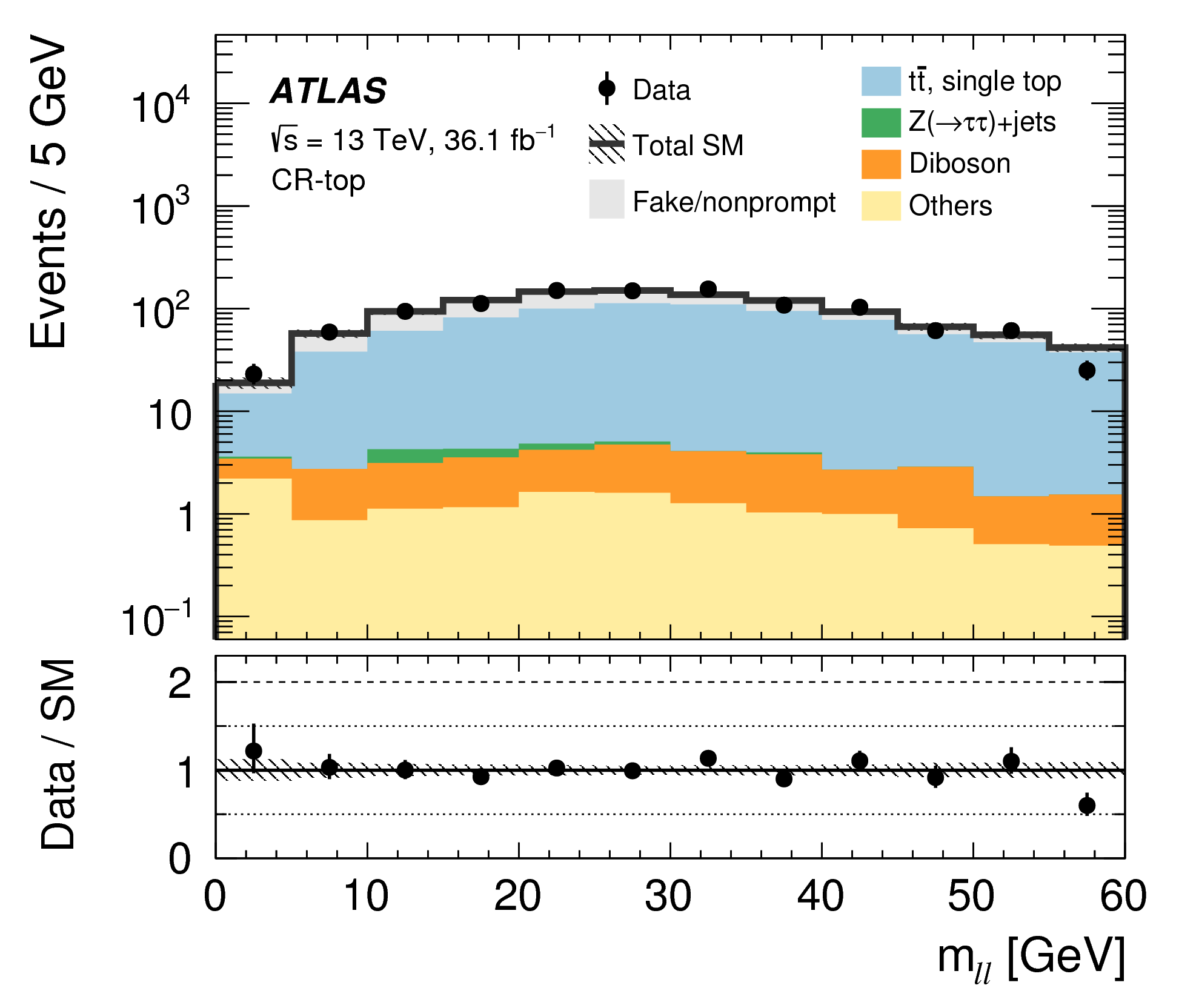
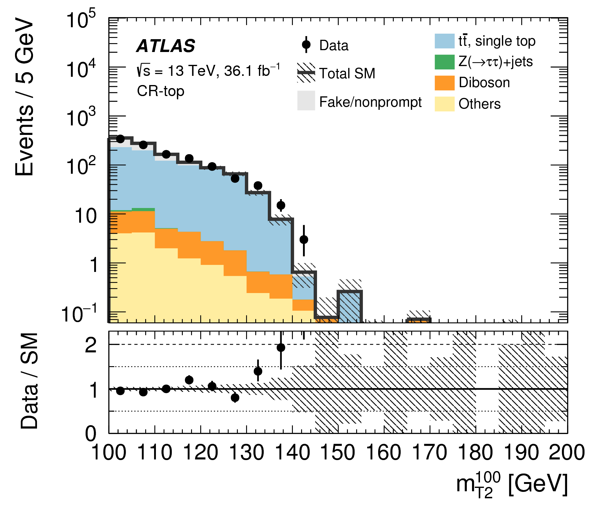
Figure 15a: Distributions after the background-only fit of the control regions. The category `Others' contains rare backgrounds from triboson, Higgs boson, and the remaining top-quark production processes listed in Table 1. The last bin includes overflow. The blue arrow indicates the final requirement used to define the selection. png (81kB) pdf (16kB)
Figure 15b: Distributions after the background-only fit of the control regions. The category `Others' contains rare backgrounds from triboson, Higgs boson, and the remaining top-quark production processes listed in Table 1. The last bin includes overflow. The blue arrow indicates the final requirement used to define the selection. png (50kB) pdf (17kB)
Figure 15c: Distributions after the background-only fit of the control regions. The category `Others' contains rare backgrounds from triboson, Higgs boson, and the remaining top-quark production processes listed in Table 1. The last bin includes overflow. The blue arrow indicates the final requirement used to define the selection. png (44kB) pdf (18kB)
Figure 15d: Distributions after the background-only fit of the control regions. The category `Others' contains rare backgrounds from triboson, Higgs boson, and the remaining top-quark production processes listed in Table 1. The last bin includes overflow. The blue arrow indicates the final requirement used to define the selection. png (52kB) pdf (18kB)
Figure 15e: Distributions after the background-only fit of the control regions. The category `Others' contains rare backgrounds from triboson, Higgs boson, and the remaining top-quark production processes listed in Table 1. The last bin includes overflow. The blue arrow indicates the final requirement used to define the selection. png (51kB) pdf (17kB)
Figure 15f: Distributions after the background-only fit of the control regions. The category `Others' contains rare backgrounds from triboson, Higgs boson, and the remaining top-quark production processes listed in Table 1. The last bin includes overflow. The blue arrow indicates the final requirement used to define the selection. png (50kB) pdf (17kB)
Figure 16a: Distributions after the background-only fit in validation regions. The category `Others' contains rare backgrounds from triboson, Higgs boson, and the remaining top-quark production processes listed in Table 1. The last bin includes overflow. The blue arrow in the E_T^miss / H_T^lep distributions indicates the minimum value of the final requirement used to define the selection. Orange arrows in the Data/SM panel indicate values that are beyond the y-axis range. png (85kB) pdf (18kB)
Figure 16b: Distributions after the background-only fit in validation regions. The category `Others' contains rare backgrounds from triboson, Higgs boson, and the remaining top-quark production processes listed in Table 1. The last bin includes overflow. The blue arrow in the E_T^miss / H_T^lep distributions indicates the minimum value of the final requirement used to define the selection. Orange arrows in the Data/SM panel indicate values that are beyond the y-axis range. png (49kB) pdf (17kB)
Figure 16c: Distributions after the background-only fit in validation regions. The category `Others' contains rare backgrounds from triboson, Higgs boson, and the remaining top-quark production processes listed in Table 1. The last bin includes overflow. The blue arrow in the E_T^miss / H_T^lep distributions indicates the minimum value of the final requirement used to define the selection. Orange arrows in the Data/SM panel indicate values that are beyond the y-axis range. png (84kB) pdf (17kB)
Figure 16d: Distributions after the background-only fit in validation regions. The category `Others' contains rare backgrounds from triboson, Higgs boson, and the remaining top-quark production processes listed in Table 1. The last bin includes overflow. The blue arrow in the E_T^miss / H_T^lep distributions indicates the minimum value of the final requirement used to define the selection. Orange arrows in the Data/SM panel indicate values that are beyond the y-axis range. png (52kB) pdf (18kB)
Figure 16e: Distributions after the background-only fit in validation regions. The category `Others' contains rare backgrounds from triboson, Higgs boson, and the remaining top-quark production processes listed in Table 1. The last bin includes overflow. The blue arrow in the E_T^miss / H_T^lep distributions indicates the minimum value of the final requirement used to define the selection. Orange arrows in the Data/SM panel indicate values that are beyond the y-axis range. png (101kB) pdf (19kB)
Figure 16f: Distributions after the background-only fit in validation regions. The category `Others' contains rare backgrounds from triboson, Higgs boson, and the remaining top-quark production processes listed in Table 1. The last bin includes overflow. The blue arrow in the E_T^miss / H_T^lep distributions indicates the minimum value of the final requirement used to define the selection. Orange arrows in the Data/SM panel indicate values that are beyond the y-axis range. png (109kB) pdf (21kB)
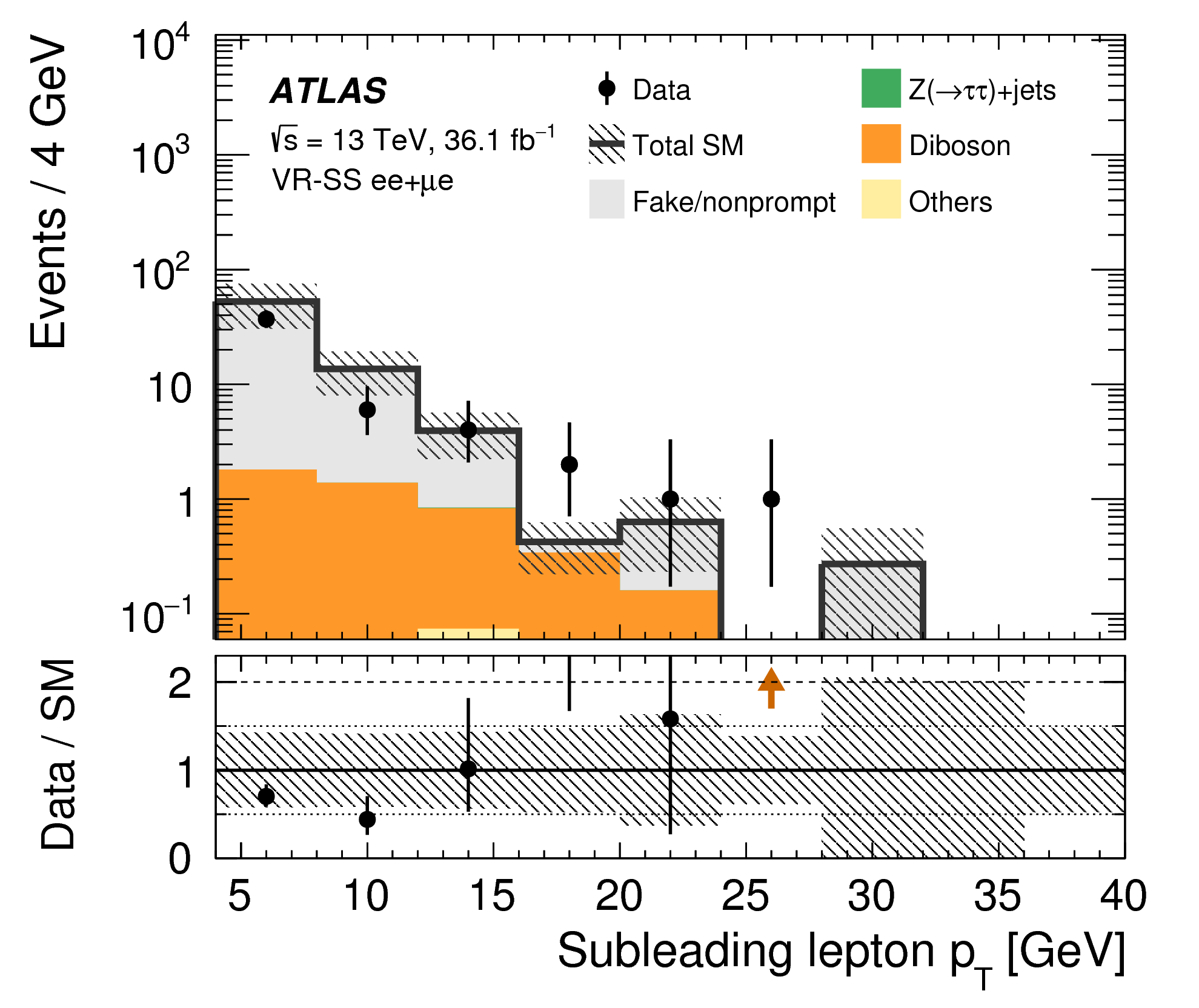
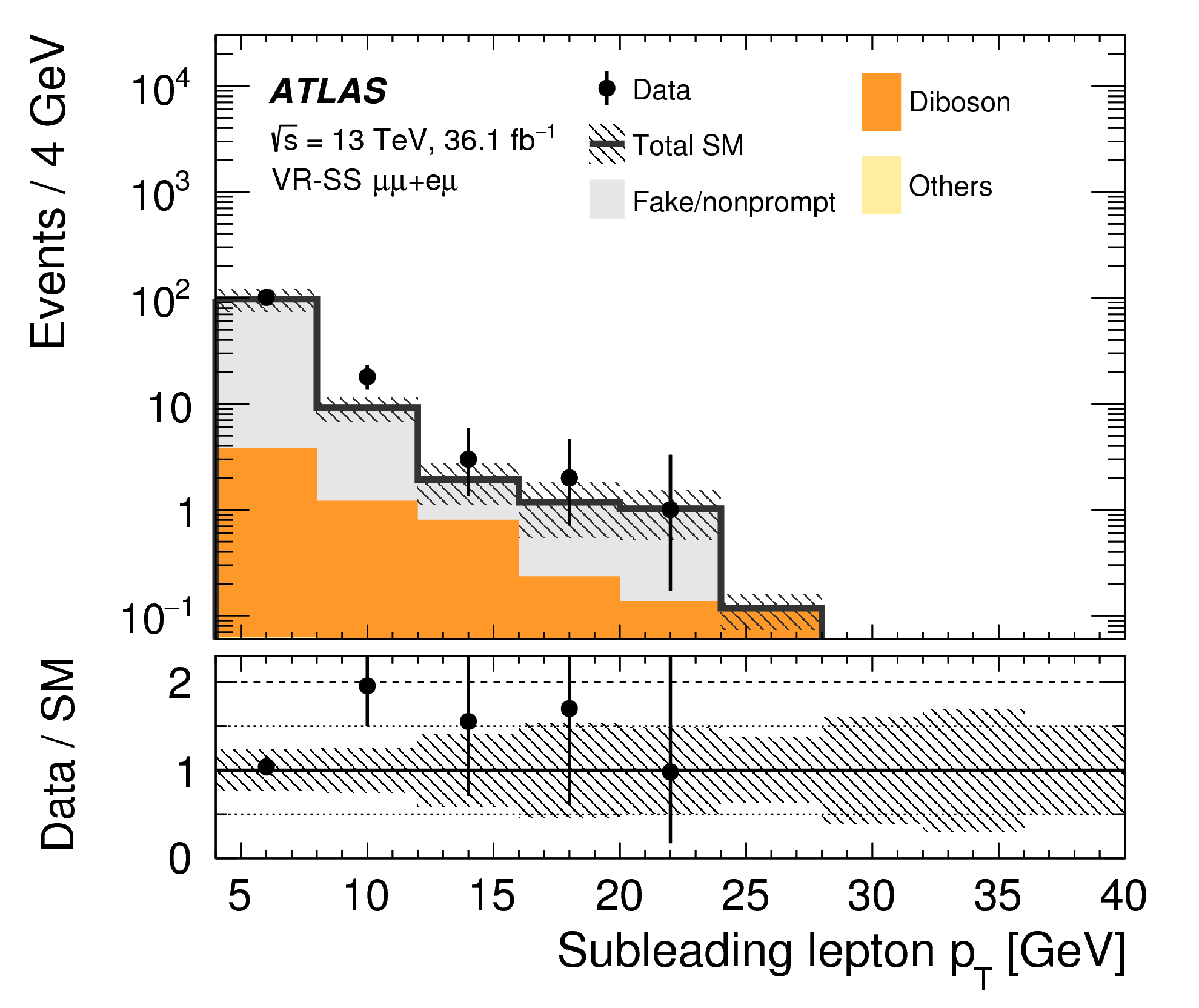
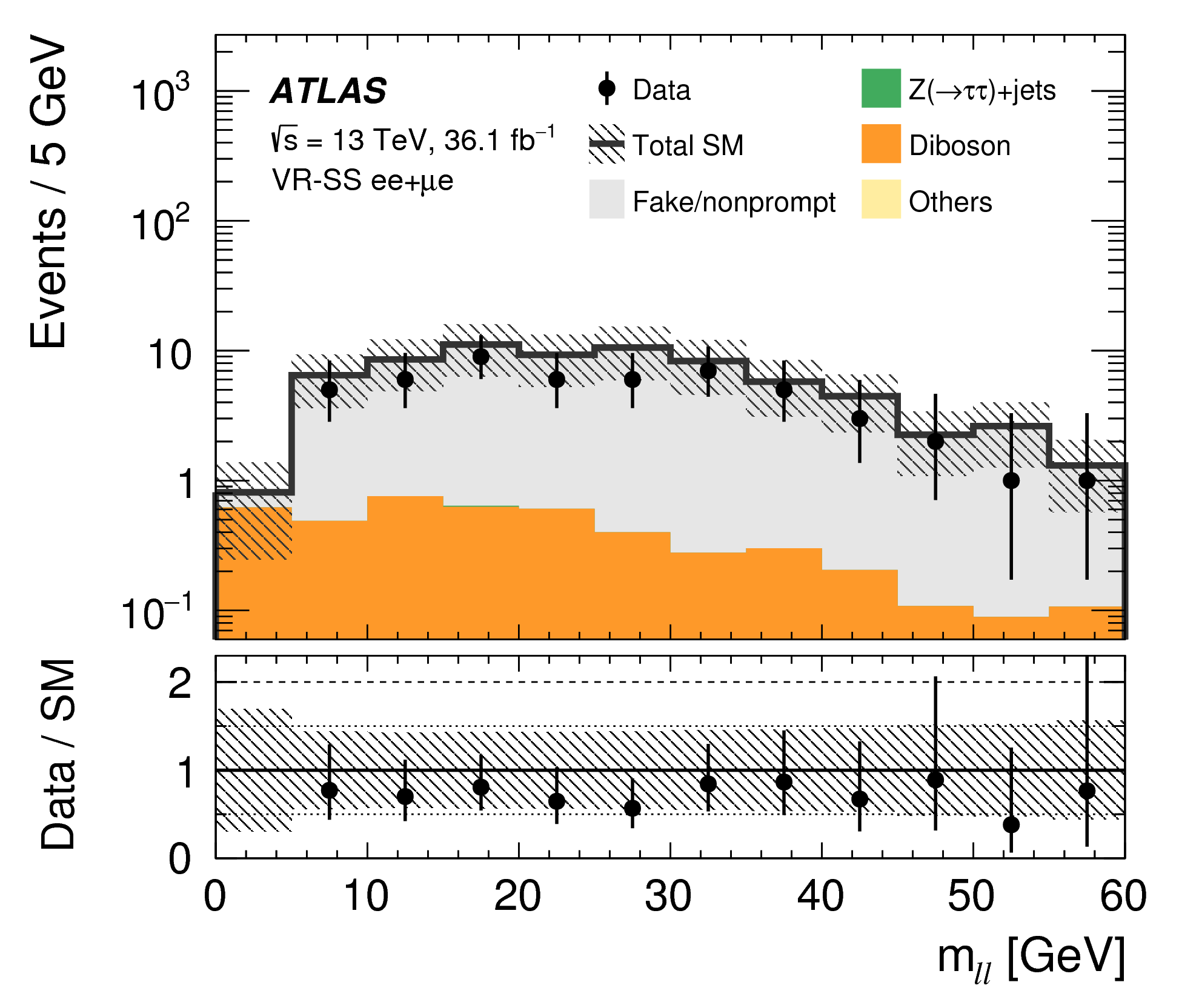
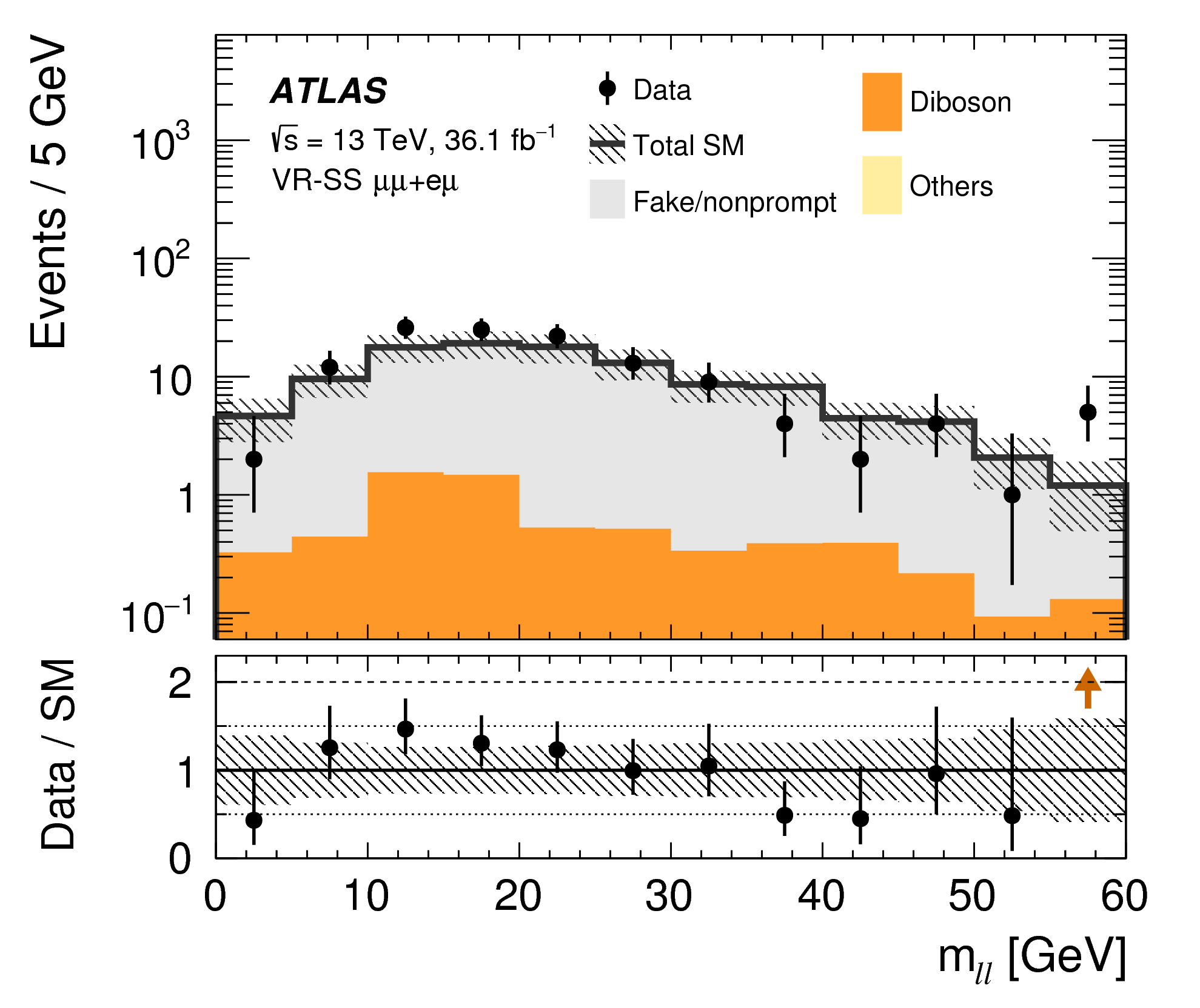
Figure 17a: Distributions after the background-only fit for the same-sign validation regions, where the subleading lepton is either the electron ee+μ e or muon μμ + eμ. The category `Others' contains rare backgrounds from triboson, Higgs boson, and the remaining top-quark production processes listed in Table 1. The last bin includes overflow. Orange arrows in the Data/SM panel indicate values that are beyond the y-axis range. png (50kB) pdf (17kB)
Figure 17b: Distributions after the background-only fit for the same-sign validation regions, where the subleading lepton is either the electron ee+μ e or muon μμ + eμ. The category `Others' contains rare backgrounds from triboson, Higgs boson, and the remaining top-quark production processes listed in Table 1. The last bin includes overflow. Orange arrows in the Data/SM panel indicate values that are beyond the y-axis range. png (47kB) pdf (17kB)
Figure 17c: Distributions after the background-only fit for the same-sign validation regions, where the subleading lepton is either the electron ee+μ e or muon μμ + eμ. The category `Others' contains rare backgrounds from triboson, Higgs boson, and the remaining top-quark production processes listed in Table 1. The last bin includes overflow. Orange arrows in the Data/SM panel indicate values that are beyond the y-axis range. png (50kB) pdf (17kB)
Figure 17d: Distributions after the background-only fit for the same-sign validation regions, where the subleading lepton is either the electron ee+μ e or muon μμ + eμ. The category `Others' contains rare backgrounds from triboson, Higgs boson, and the remaining top-quark production processes listed in Table 1. The last bin includes overflow. Orange arrows in the Data/SM panel indicate values that are beyond the y-axis range. png (47kB) pdf (18kB)
Figure 17e: Distributions after the background-only fit for the same-sign validation regions, where the subleading lepton is either the electron ee+μ e or muon μμ + eμ. The category `Others' contains rare backgrounds from triboson, Higgs boson, and the remaining top-quark production processes listed in Table 1. The last bin includes overflow. Orange arrows in the Data/SM panel indicate values that are beyond the y-axis range. png (46kB) pdf (17kB)
Figure 17f: Distributions after the background-only fit for the same-sign validation regions, where the subleading lepton is either the electron ee+μ e or muon μμ + eμ. The category `Others' contains rare backgrounds from triboson, Higgs boson, and the remaining top-quark production processes listed in Table 1. The last bin includes overflow. Orange arrows in the Data/SM panel indicate values that are beyond the y-axis range. png (50kB) pdf (17kB)
Figure 18: Distributions after the background-only fit for the same-sign validation region. The category `Others' contains rare backgrounds from triboson, Higgs boson, and the remaining top-quark production processes listed in Table 1. The last bin includes overflow. Orange arrows in the Data/SM panel indicate values that are beyond the y-axis range. png (52kB) pdf (18kB)
Figure 19a: Distributions after the exclusion fit to the SRℓℓ-m_ℓℓ signal regions with the signal strength parameter set to zero. The category `Others' contains rare backgrounds from triboson, Higgs boson, and the remaining top-quark production processes listed in Table 1. The last bin includes overflow. The blue arrow in the E_T^miss / H_T^lep distribution indicates the minimum value of the final requirement used to define the selection. Benchmark Higgsino H̃ signals are overlaid as dashed lines. png (113kB) pdf (18kB)
Figure 19b: Distributions after the exclusion fit to the SRℓℓ-m_ℓℓ signal regions with the signal strength parameter set to zero. The category `Others' contains rare backgrounds from triboson, Higgs boson, and the remaining top-quark production processes listed in Table 1. The last bin includes overflow. The blue arrow in the E_T^miss / H_T^lep distribution indicates the minimum value of the final requirement used to define the selection. Benchmark Higgsino H̃ signals are overlaid as dashed lines. png (110kB) pdf (18kB)
Figure 20a: Distributions after the exclusion fit to the SRℓℓ-m_T2¹⁰⁰ signal regions with the signal strength parameter set to zero. The category `Others' contains rare backgrounds from triboson, Higgs boson, and the remaining top-quark production processes listed in Table 1. The last bin includes overflow. The blue arrow in the E_T^miss / H_T^lep distribution indicates the minimum value of the final requirement used to define the selection. Benchmark slepton ℓ̃ signals are overlaid as dashed lines. Orange arrows in the Data/SM panel indicate values that are beyond the y-axis range. png (135kB) pdf (22kB)
Figure 20b: Distributions after the exclusion fit to the SRℓℓ-m_T2¹⁰⁰ signal regions with the signal strength parameter set to zero. The category `Others' contains rare backgrounds from triboson, Higgs boson, and the remaining top-quark production processes listed in Table 1. The last bin includes overflow. The blue arrow in the E_T^miss / H_T^lep distribution indicates the minimum value of the final requirement used to define the selection. Benchmark slepton ℓ̃ signals are overlaid as dashed lines. Orange arrows in the Data/SM panel indicate values that are beyond the y-axis range. png (115kB) pdf (19kB)
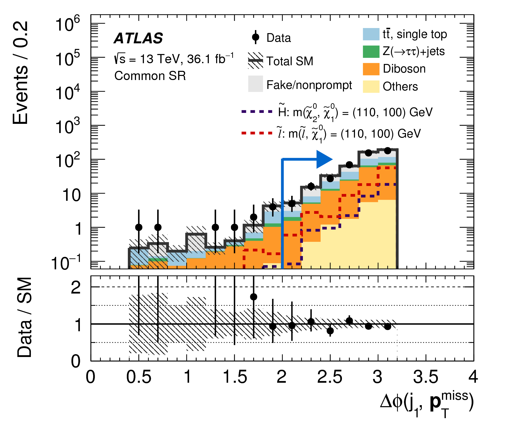
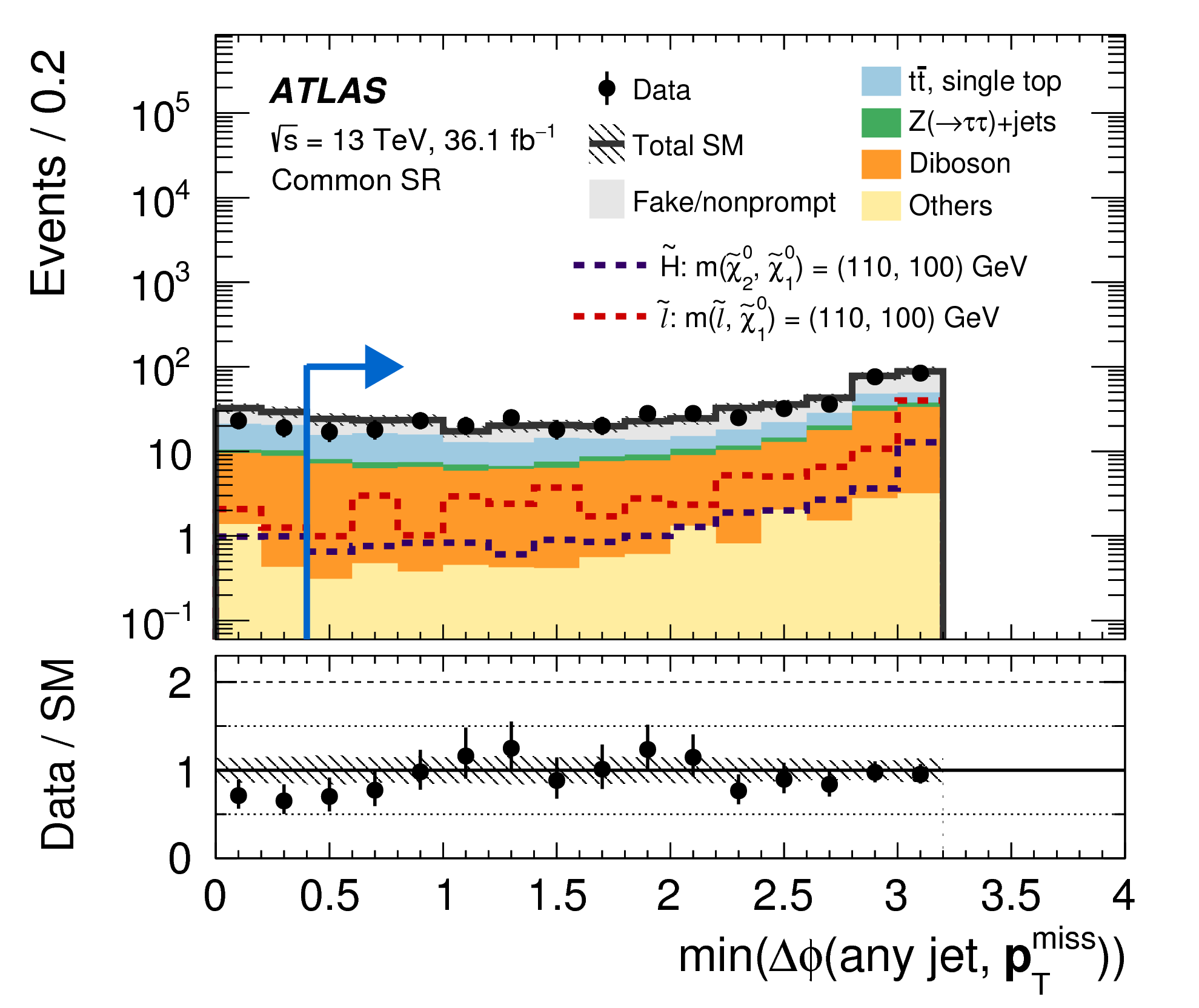
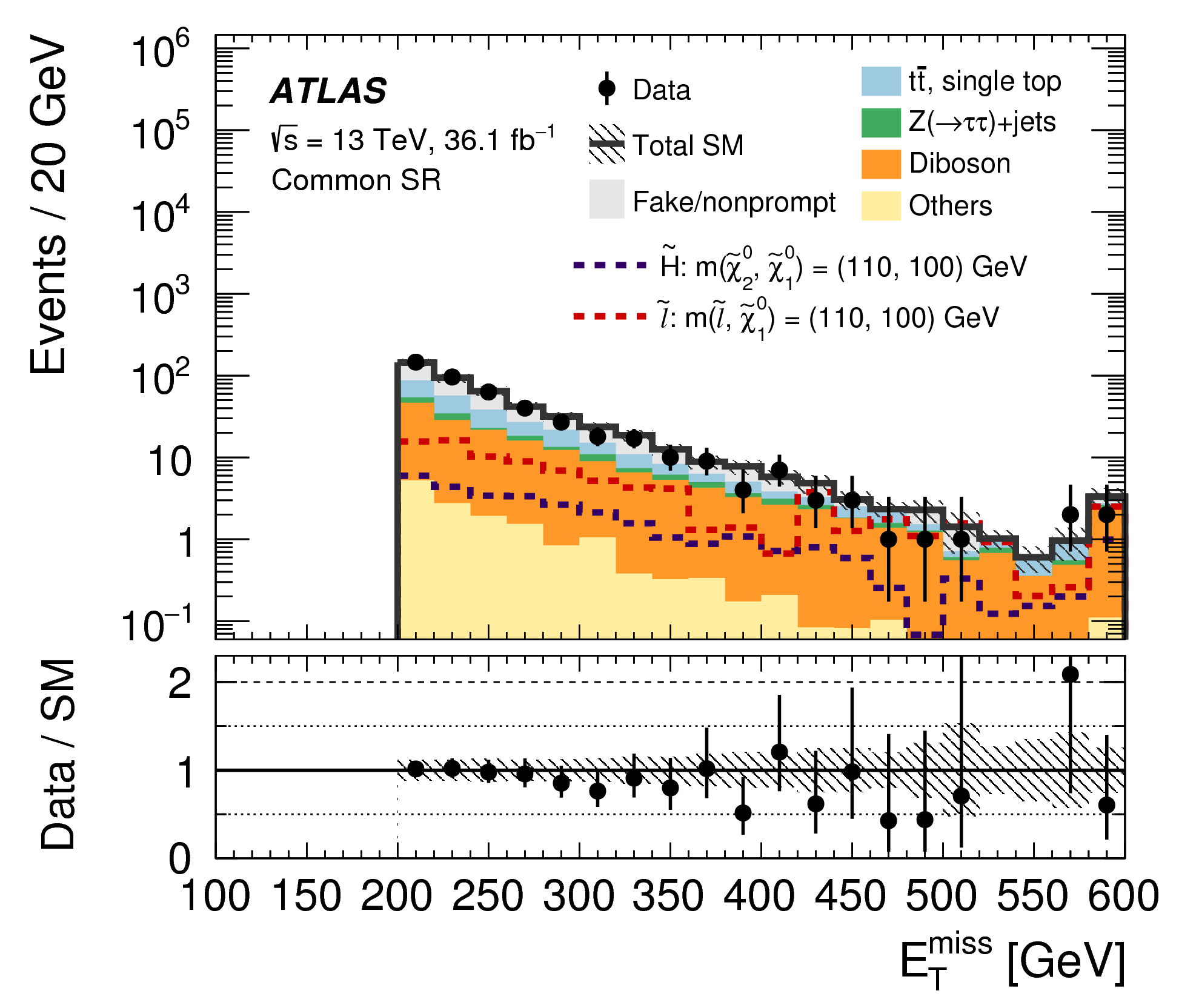
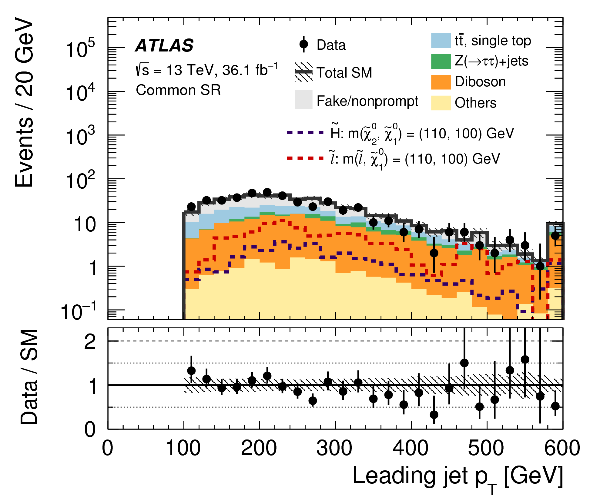
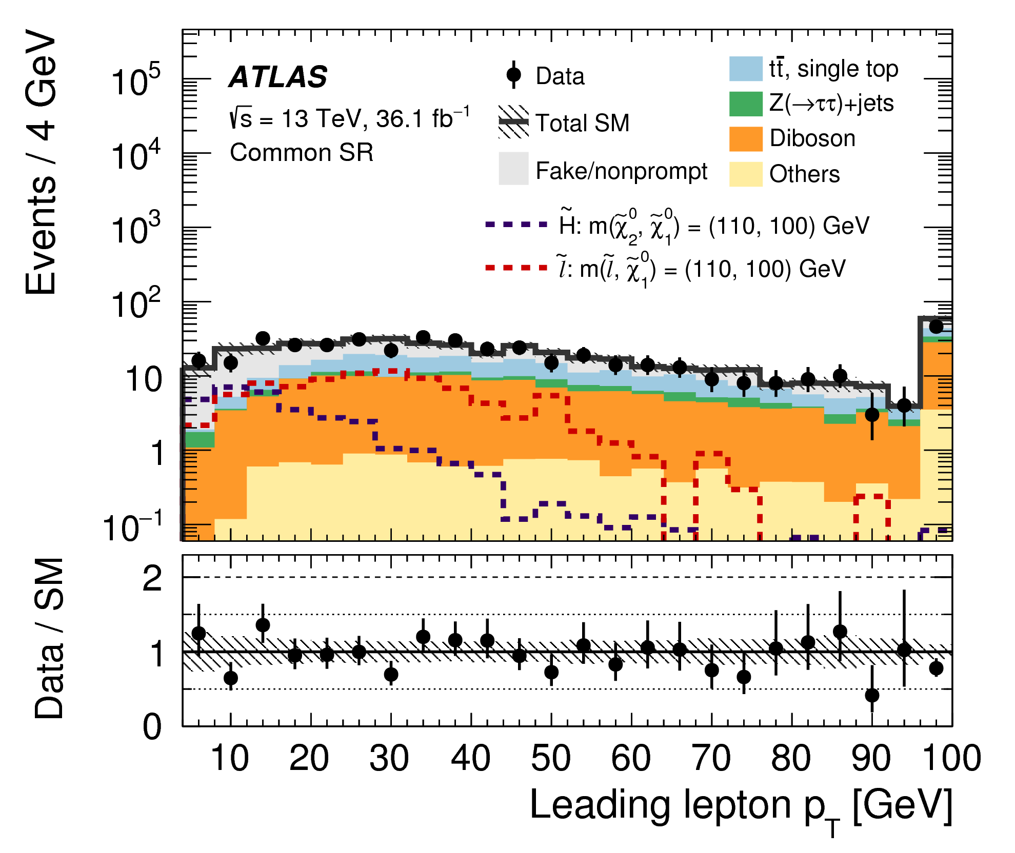
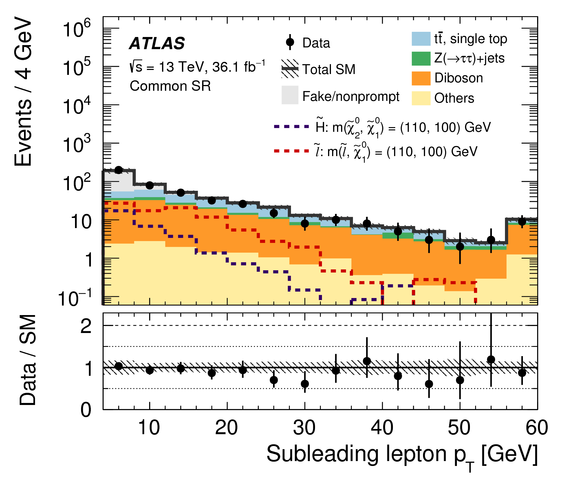
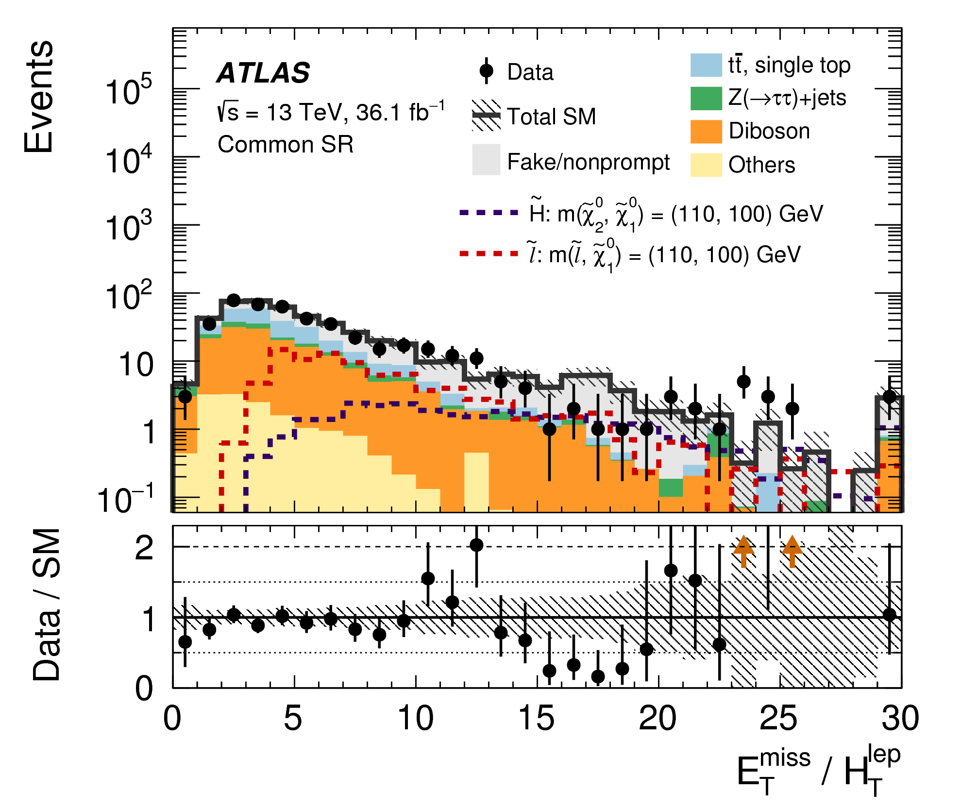
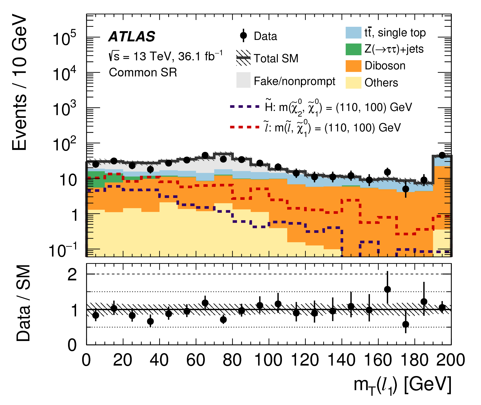
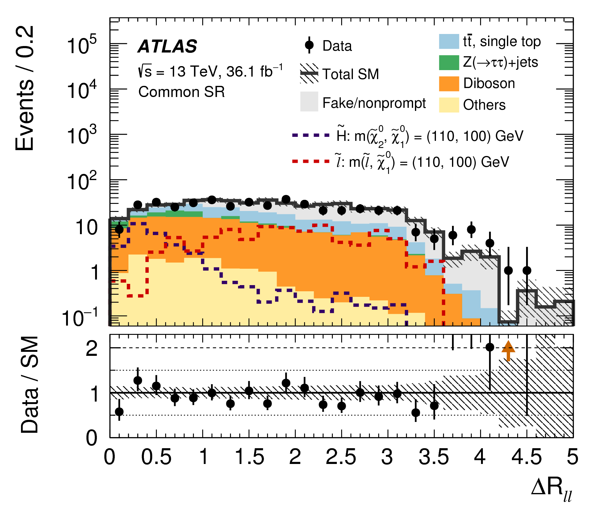
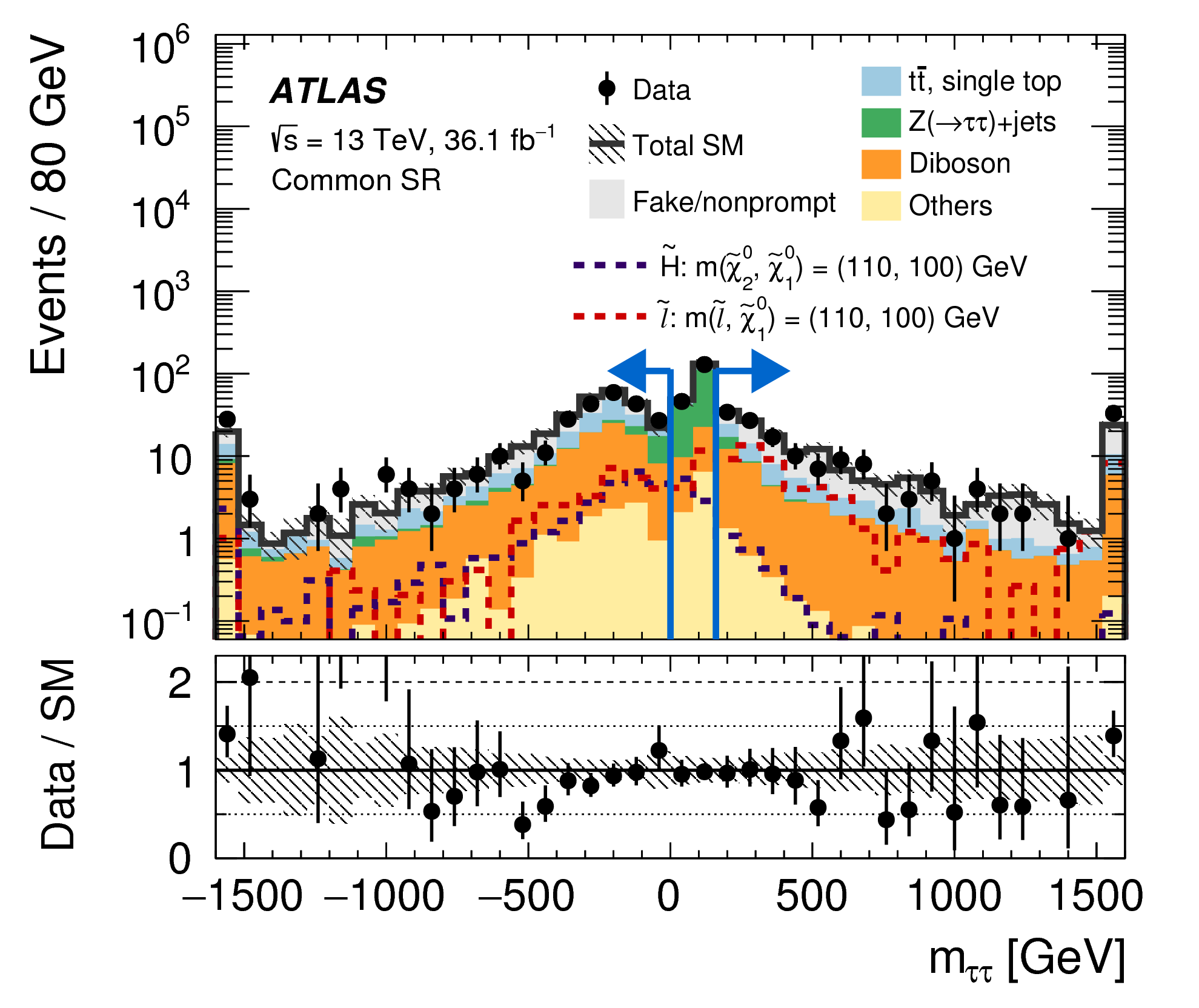
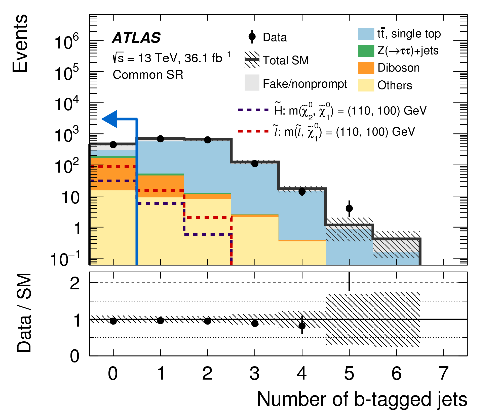
Figure 21a: Distributions after the background-only fit of kinematic variables used to define selections common to all signal regions, i.e. not including requirements specific to the electroweakino or slepton SR definitions. Blue arrows in the upper panel denote the final requirement used to define the common SR, otherwise all selections are applied. The category `Others' contains rare backgrounds from triboson, Higgs boson, and the remaining top-quark production processes listed in Table 1. The first (last) bin includes underflow (overflow). Benchmark Higgsino H̃ and slepton ℓ̃ signals are overlaid as dashed lines. Orange arrows in the Data/SM panel indicate values that are beyond the y-axis range. png (110kB) pdf (19kB)
Figure 21b: Distributions after the background-only fit of kinematic variables used to define selections common to all signal regions, i.e. not including requirements specific to the electroweakino or slepton SR definitions. Blue arrows in the upper panel denote the final requirement used to define the common SR, otherwise all selections are applied. The category `Others' contains rare backgrounds from triboson, Higgs boson, and the remaining top-quark production processes listed in Table 1. The first (last) bin includes underflow (overflow). Benchmark Higgsino H̃ and slepton ℓ̃ signals are overlaid as dashed lines. Orange arrows in the Data/SM panel indicate values that are beyond the y-axis range. png (111kB) pdf (20kB)
Figure 21c: Distributions after the background-only fit of kinematic variables used to define selections common to all signal regions, i.e. not including requirements specific to the electroweakino or slepton SR definitions. Blue arrows in the upper panel denote the final requirement used to define the common SR, otherwise all selections are applied. The category `Others' contains rare backgrounds from triboson, Higgs boson, and the remaining top-quark production processes listed in Table 1. The first (last) bin includes underflow (overflow). Benchmark Higgsino H̃ and slepton ℓ̃ signals are overlaid as dashed lines. Orange arrows in the Data/SM panel indicate values that are beyond the y-axis range. png (122kB) pdf (21kB)
Figure 21d: Distributions after the background-only fit of kinematic variables used to define selections common to all signal regions, i.e. not including requirements specific to the electroweakino or slepton SR definitions. Blue arrows in the upper panel denote the final requirement used to define the common SR, otherwise all selections are applied. The category `Others' contains rare backgrounds from triboson, Higgs boson, and the remaining top-quark production processes listed in Table 1. The first (last) bin includes underflow (overflow). Benchmark Higgsino H̃ and slepton ℓ̃ signals are overlaid as dashed lines. Orange arrows in the Data/SM panel indicate values that are beyond the y-axis range. png (125kB) pdf (21kB)
Figure 21e: Distributions after the background-only fit of kinematic variables used to define selections common to all signal regions, i.e. not including requirements specific to the electroweakino or slepton SR definitions. Blue arrows in the upper panel denote the final requirement used to define the common SR, otherwise all selections are applied. The category `Others' contains rare backgrounds from triboson, Higgs boson, and the remaining top-quark production processes listed in Table 1. The first (last) bin includes underflow (overflow). Benchmark Higgsino H̃ and slepton ℓ̃ signals are overlaid as dashed lines. Orange arrows in the Data/SM panel indicate values that are beyond the y-axis range. png (123kB) pdf (23kB)
Figure 21f: Distributions after the background-only fit of kinematic variables used to define selections common to all signal regions, i.e. not including requirements specific to the electroweakino or slepton SR definitions. Blue arrows in the upper panel denote the final requirement used to define the common SR, otherwise all selections are applied. The category `Others' contains rare backgrounds from triboson, Higgs boson, and the remaining top-quark production processes listed in Table 1. The first (last) bin includes underflow (overflow). Benchmark Higgsino H̃ and slepton ℓ̃ signals are overlaid as dashed lines. Orange arrows in the Data/SM panel indicate values that are beyond the y-axis range. png (112kB) pdf (19kB)
Figure 21g: Distributions after the background-only fit of kinematic variables used to define selections common to all signal regions, i.e. not including requirements specific to the electroweakino or slepton SR definitions. Blue arrows in the upper panel denote the final requirement used to define the common SR, otherwise all selections are applied. The category `Others' contains rare backgrounds from triboson, Higgs boson, and the remaining top-quark production processes listed in Table 1. The first (last) bin includes underflow (overflow). Benchmark Higgsino H̃ and slepton ℓ̃ signals are overlaid as dashed lines. Orange arrows in the Data/SM panel indicate values that are beyond the y-axis range. png (131kB) pdf (23kB)
Figure 21h: Distributions after the background-only fit of kinematic variables used to define selections common to all signal regions, i.e. not including requirements specific to the electroweakino or slepton SR definitions. Blue arrows in the upper panel denote the final requirement used to define the common SR, otherwise all selections are applied. The category `Others' contains rare backgrounds from triboson, Higgs boson, and the remaining top-quark production processes listed in Table 1. The first (last) bin includes underflow (overflow). Benchmark Higgsino H̃ and slepton ℓ̃ signals are overlaid as dashed lines. Orange arrows in the Data/SM panel indicate values that are beyond the y-axis range. png (117kB) pdf (21kB)
Figure 21i: Distributions after the background-only fit of kinematic variables used to define selections common to all signal regions, i.e. not including requirements specific to the electroweakino or slepton SR definitions. Blue arrows in the upper panel denote the final requirement used to define the common SR, otherwise all selections are applied. The category `Others' contains rare backgrounds from triboson, Higgs boson, and the remaining top-quark production processes listed in Table 1. The first (last) bin includes underflow (overflow). Benchmark Higgsino H̃ and slepton ℓ̃ signals are overlaid as dashed lines. Orange arrows in the Data/SM panel indicate values that are beyond the y-axis range. png (120kB) pdf (21kB)
Figure 21j: Distributions after the background-only fit of kinematic variables used to define selections common to all signal regions, i.e. not including requirements specific to the electroweakino or slepton SR definitions. Blue arrows in the upper panel denote the final requirement used to define the common SR, otherwise all selections are applied. The category `Others' contains rare backgrounds from triboson, Higgs boson, and the remaining top-quark production processes listed in Table 1. The first (last) bin includes underflow (overflow). Benchmark Higgsino H̃ and slepton ℓ̃ signals are overlaid as dashed lines. Orange arrows in the Data/SM panel indicate values that are beyond the y-axis range. png (146kB) pdf (25kB)
Figure 21k: Distributions after the background-only fit of kinematic variables used to define selections common to all signal regions, i.e. not including requirements specific to the electroweakino or slepton SR definitions. Blue arrows in the upper panel denote the final requirement used to define the common SR, otherwise all selections are applied. The category `Others' contains rare backgrounds from triboson, Higgs boson, and the remaining top-quark production processes listed in Table 1. The first (last) bin includes underflow (overflow). Benchmark Higgsino H̃ and slepton ℓ̃ signals are overlaid as dashed lines. Orange arrows in the Data/SM panel indicate values that are beyond the y-axis range. png (101kB) pdf (17kB)
Figure 22: Comparison of expected and observed event yields in the inclusive signal regions after the background-only fit. Background processes containing fewer than two prompt leptons are categorized as `Fake/nonprompt'. The category `Others' contains rare backgrounds from triboson, Higgs boson, and the remaining top-quark production processes listed in Table 1. Uncertainties in the background estimates include both the statistical and systematic uncertainties, where σ_tot denotes the total uncertainty. png (23kB) pdf (19kB)
Figure 23a: Numbers show the CLs values in the Higgsino simplified model. png (57kB) pdf (291kB)
Figure 23b: Numbers show the CLs values in the Higgsino simplified model. png (57kB) pdf (291kB)
Figure 24a: Numbers show the CLs values in the wino--bino simplified model. png (65kB) pdf (296kB)
Figure 24b: Numbers show the CLs values in the wino--bino simplified model. png (65kB) pdf (296kB)
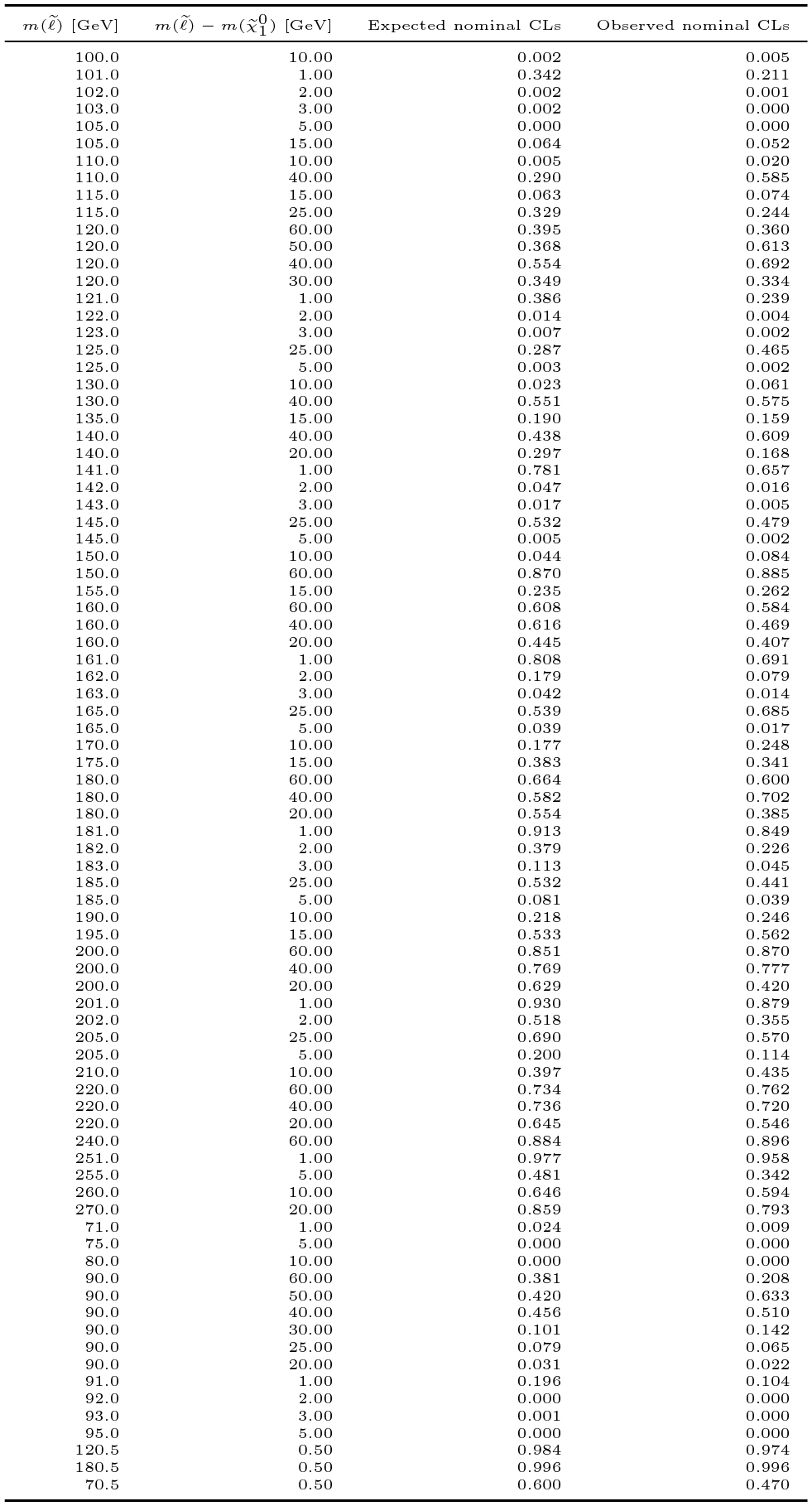
Figure 25a: Numbers show the CLs values in the slepton simplified model. png (63kB) pdf (262kB)
Figure 25b: Numbers show the CLs values in the slepton simplified model. png (63kB) pdf (262kB)
Figure 26a: Numbers show 95% CL model-dependent upper limits on the inclusive Higgsino signal cross-sections. png (56kB) pdf (292kB)
Figure 26b: Numbers show 95% CL model-dependent upper limits on the inclusive Higgsino signal cross-sections. png (56kB) pdf (292kB)
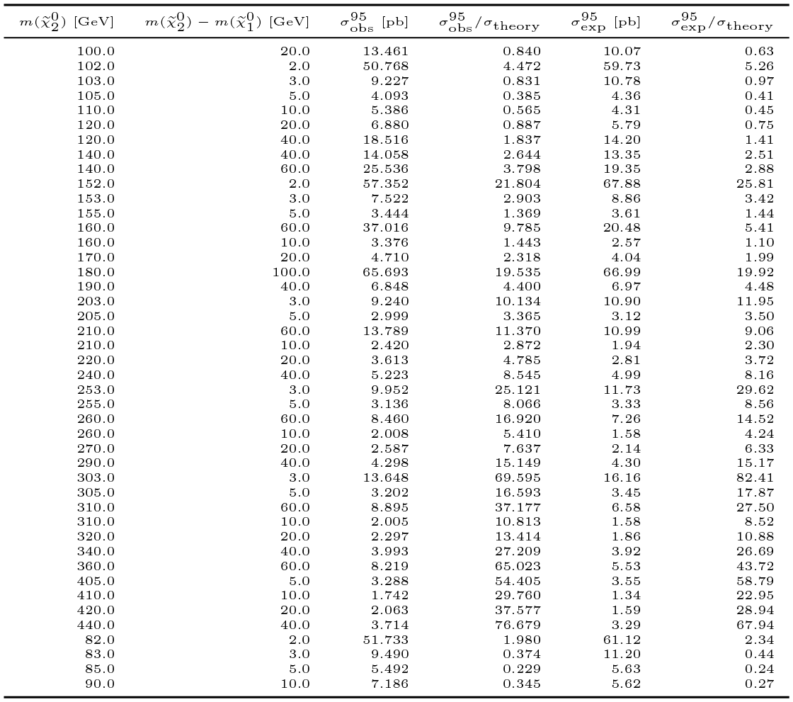
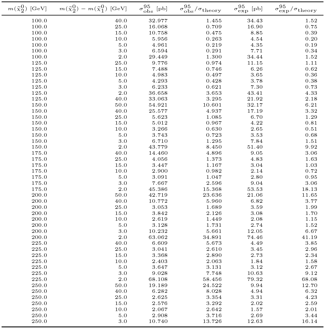
Figure 27a: Numbers show 95% CL model-dependent upper limits on the inclusive signal cross-sections of the wino--bino model. png (63kB) pdf (297kB)
Figure 27b: Numbers show 95% CL model-dependent upper limits on the inclusive signal cross-sections of the wino--bino model. png (63kB) pdf (297kB)
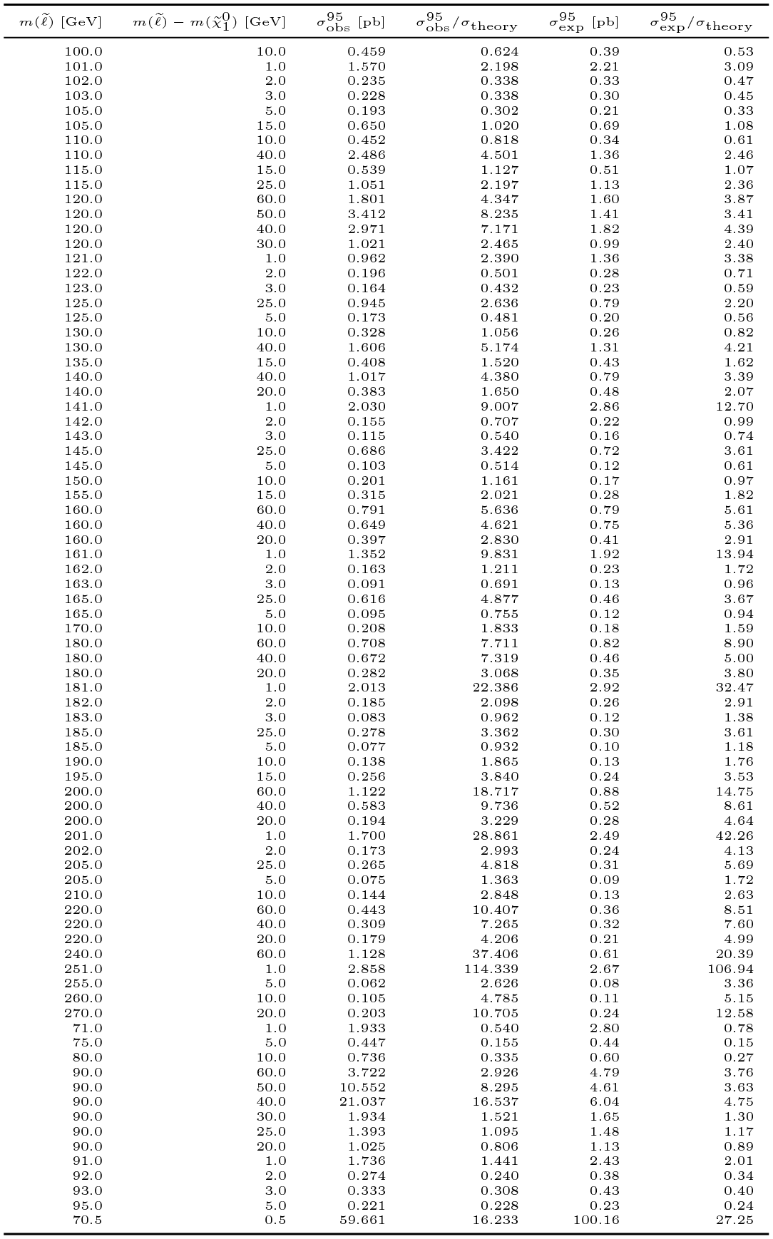
Figure 28a: Numbers show the 95% CL model-dependent upper limits on the slepton signal cross-sections, assuming a fourfold mass degeneracy m(ẽ_L,R) = m(μ̃_L,R). png (61kB) pdf (296kB)
Figure 28b: Numbers show the 95% CL model-dependent upper limits on the slepton signal cross-sections, assuming a fourfold mass degeneracy m(ẽ_L,R) = m(μ̃_L,R). png (61kB) pdf (296kB)
Figure 29: Expected and observed 95% CL cross-section upper limits as a function of the universal gaugino mass m_1/2 for the NUHM2 model. The gray numbers indicate the values of the observed limit. The green and yellow bands around the expected limit indicate the ± 1σ and ± 2σ uncertainties, respectively. The expected signal production cross-sections as well as the associated uncertainty are indicated with the blue solid and dashed lines. The lower x-axis indicates the difference between the χ̃₂⁰ and χ̃₁⁰ masses for different values of m_1/2. A fit of signals to the m_ℓℓ spectrum is used to derive this limit. png (151kB) eps (28kB) pdf (16kB)
Figure 30a: Model-dependent exclusion limits as presented in the main text, but with a logarithmic scale for the axis labeling the mass splitting. png (52kB) pdf (256kB)
Figure 30b: Model-dependent exclusion limits as presented in the main text, but with a logarithmic scale for the axis labeling the mass splitting. png (56kB) pdf (261kB)
Figure 30c: Model-dependent exclusion limits as presented in the main text, but with a logarithmic scale for the axis labeling the mass splitting. png (52kB) pdf (260kB)
Figure 31: Higgsino simplified model exclusion limits as presented in the main text, but projected into the m(χ̃₁^±) - m(χ̃₁⁰) vs m(χ̃₁^±) plane with a logarithmic scale for the axis labeling the mass splitting. png (49kB) pdf (256kB)
Table 01: Observed event yields and exclusion fit results with the signal strength parameter set to zero for the exclusive electroweakino and slepton signal regions. Background processes containing fewer than two prompt leptons are categorized as `Fake/nonprompt'. The category `Others' contains rare backgrounds from triboson, Higgs boson, and the remaining top-quark production processes listed in Table 1. Uncertainties in the fitted background estimates combine statistical and systematic uncertainties. png (87kB) pdf (58kB)
Table 02: Observed event yields and background-only fit results for the inclusive electroweakino and slepton signal regions. Background processes containing fewer than two prompt leptons are categorized as `Fake/nonprompt'. The category `Others' contains rare backgrounds from triboson, Higgs boson, and the remaining top-quark production processes listed in Table 1. Uncertainties in the fitted background estimates combine statistical and systematic uncertainties. png (42kB) pdf (56kB)
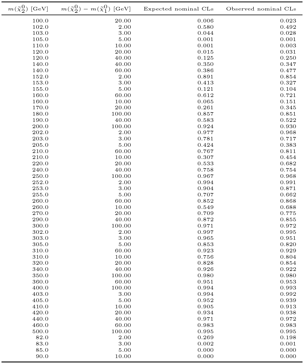
Table 03: Nominal observed and expected CLs values for Higgsino signals. png (26kB) pdf (37kB)
Table 04: Nominal observed and expected CLs values for wino--bino signals. png (22kB) pdf (37kB)
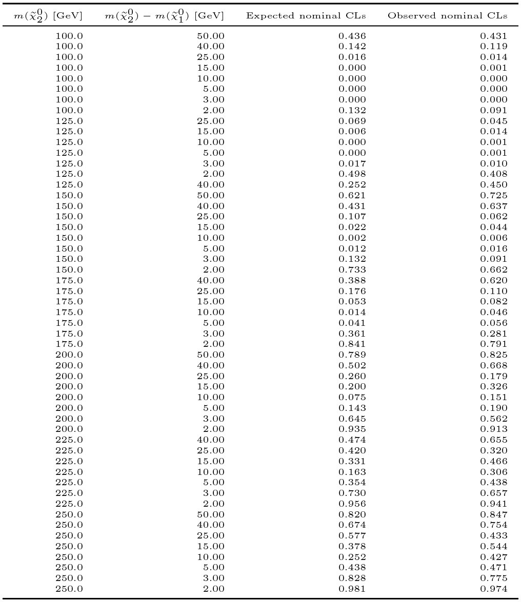
Table 05: Nominal observed and expected CLs values for slepton signals. png (35kB) pdf (37kB)
Table 06: Upper limits on observed (expected) Higgsino simplified model signal cross section σ_{obs (exp)}⁹⁵ and signal strength σ_{obs (exp)}⁹⁵ / σ_theory. png (38kB) pdf (36kB)
Table 07: Upper limits on observed (expected) wino--bino simplified model signal cross section σ_{obs (exp)}⁹⁵ and signal strength σ_{obs (exp)}⁹⁵ / σ_theory. png (40kB) pdf (36kB)
Table 08: Upper limits on observed (expected) slepton simplified model signal cross section σ_{obs (exp)}⁹⁵ and signal strength σ_{obs (exp)}⁹⁵ / σ_theory. png (57kB) pdf (37kB)
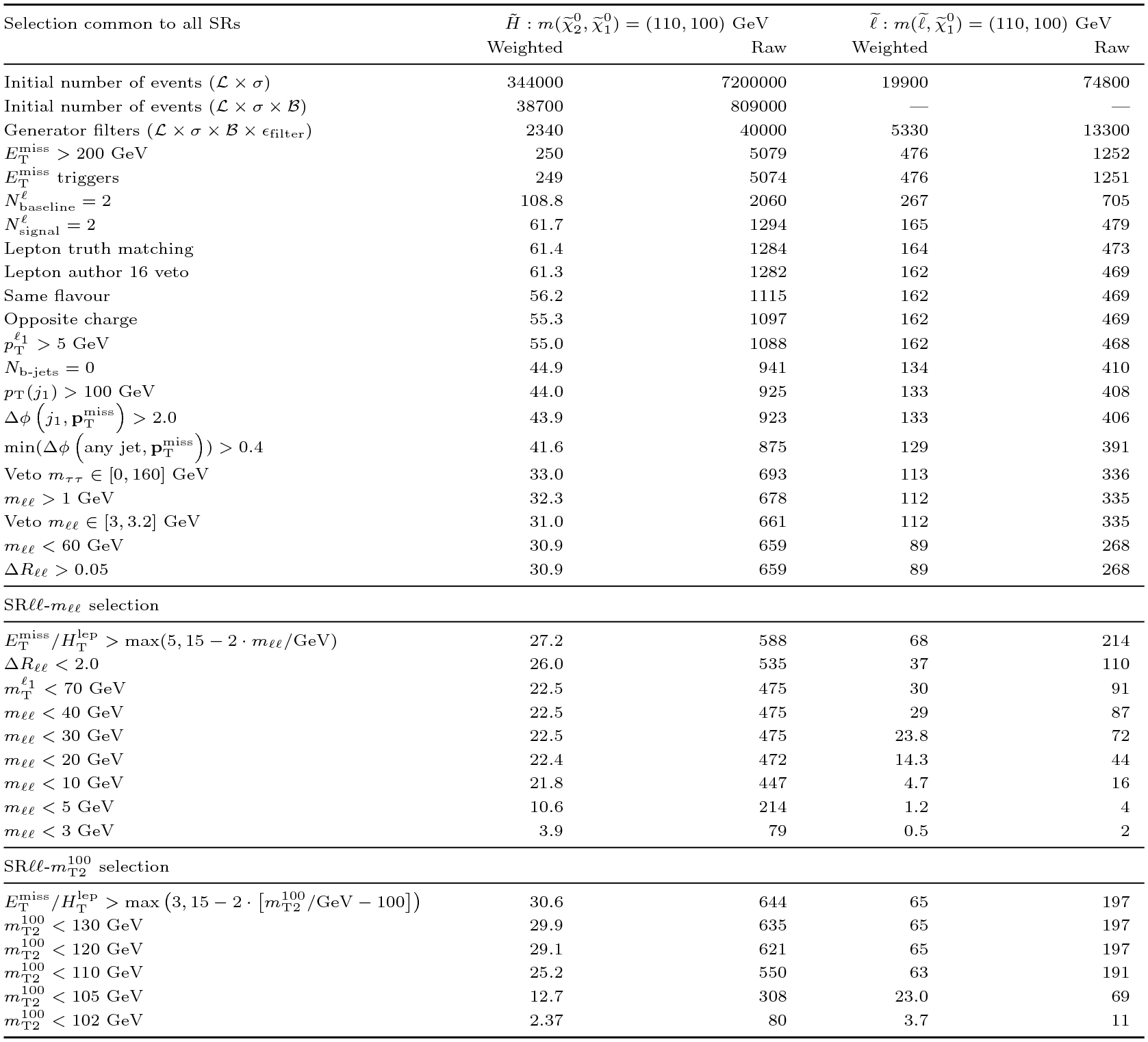
Table 09: Event counts for Higgsino H̃ and slepton ℓ̃ signals after sequential selections for the inclusive SRℓℓ-m_ℓℓ and SRℓℓ-m_T2¹⁰⁰ regions. Weighted events are normalised to mathcalL = 36.1 fb^-1 and the inclusive cross section σ, while raw MC events are also shown. The generator filter with efficiency ε_filt applied to the Higgsino signal requires truth E_T^miss > 50 GeV and at least 2 leptons with p_T > 3 GeV, while only the E_T^miss > 50 GeV requirement is applied to the slepton signal. The mathcalB refers to the branching ratio Z^(*) → ℓ⁺ℓ^- in the Higgsino processes. ``Lepton truth matching" requires that the selected leptons are consistent with being decay products of the SUSY process. ``Lepton author 16 veto" removes a class of electron candidates reconstructed with algorithms designed to identify photon conversions. png (60kB) pdf (71kB)
Table 10: Event counts for the χ̃₂⁰χ̃₁⁺ process of the Higgsino m(χ̃₂⁰, χ̃₁⁰) = (110, 100) GeV signal and sequentially with each addition requirement for selections common to all signal regions (SRs), followed by those optimised for Higgsinos and sleptons. ``Lepton truth matching" requires that the selected leptons are consistent with being decay products of the SUSY process. ``Lepton author 16 veto" removes a class of electron candidates reconstructed with algorithms designed to identify photon conversions. Weighted events are normalised to 36.1 fb^-1 and the raw Monte Carlo events are also displayed. png (45kB) pdf (71kB)
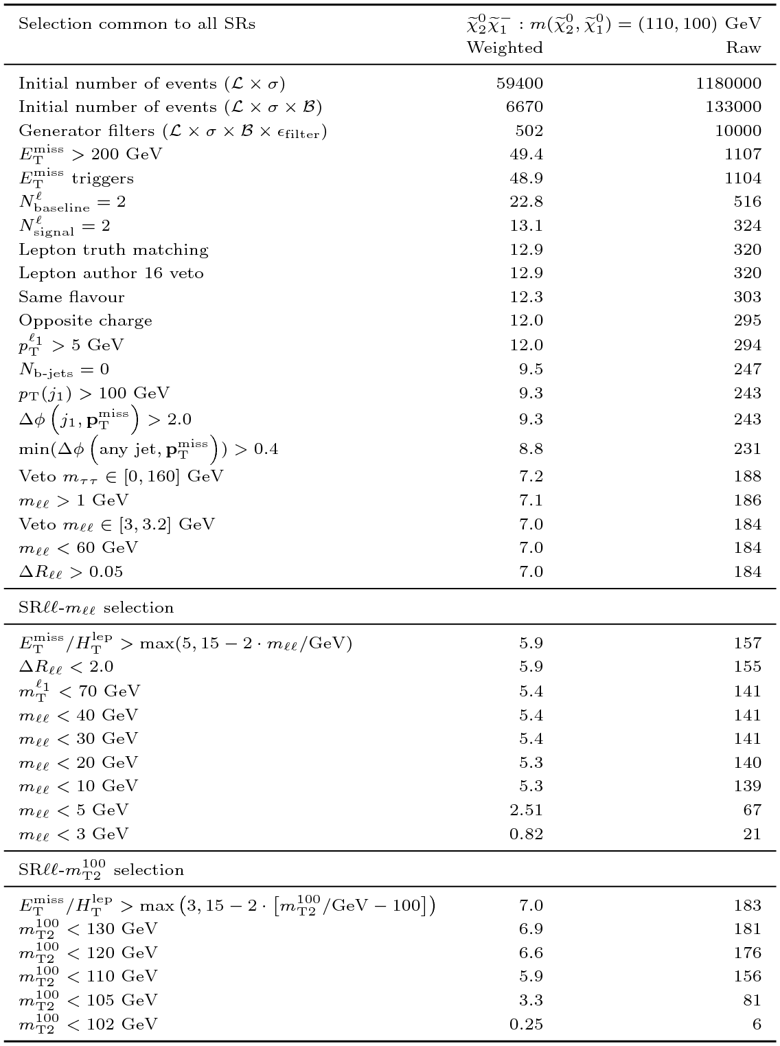
Table 11: Event counts for the χ̃₂⁰χ̃₁^- process of the Higgsino m(χ̃₂⁰, χ̃₁⁰) = (110, 100) GeV signal and sequentially with each addition requirement for selections common to all signal regions (SRs), followed by those optimised for Higgsinos and sleptons. ``Lepton truth matching" requires that the selected leptons are consistent with being decay products of the SUSY process. ``Lepton author 16 veto" removes a class of electron candidates reconstructed with algorithms designed to identify photon conversions. Weighted events are normalised to 36.1 fb^-1 and the raw Monte Carlo events are also displayed. png (44kB) pdf (78kB)
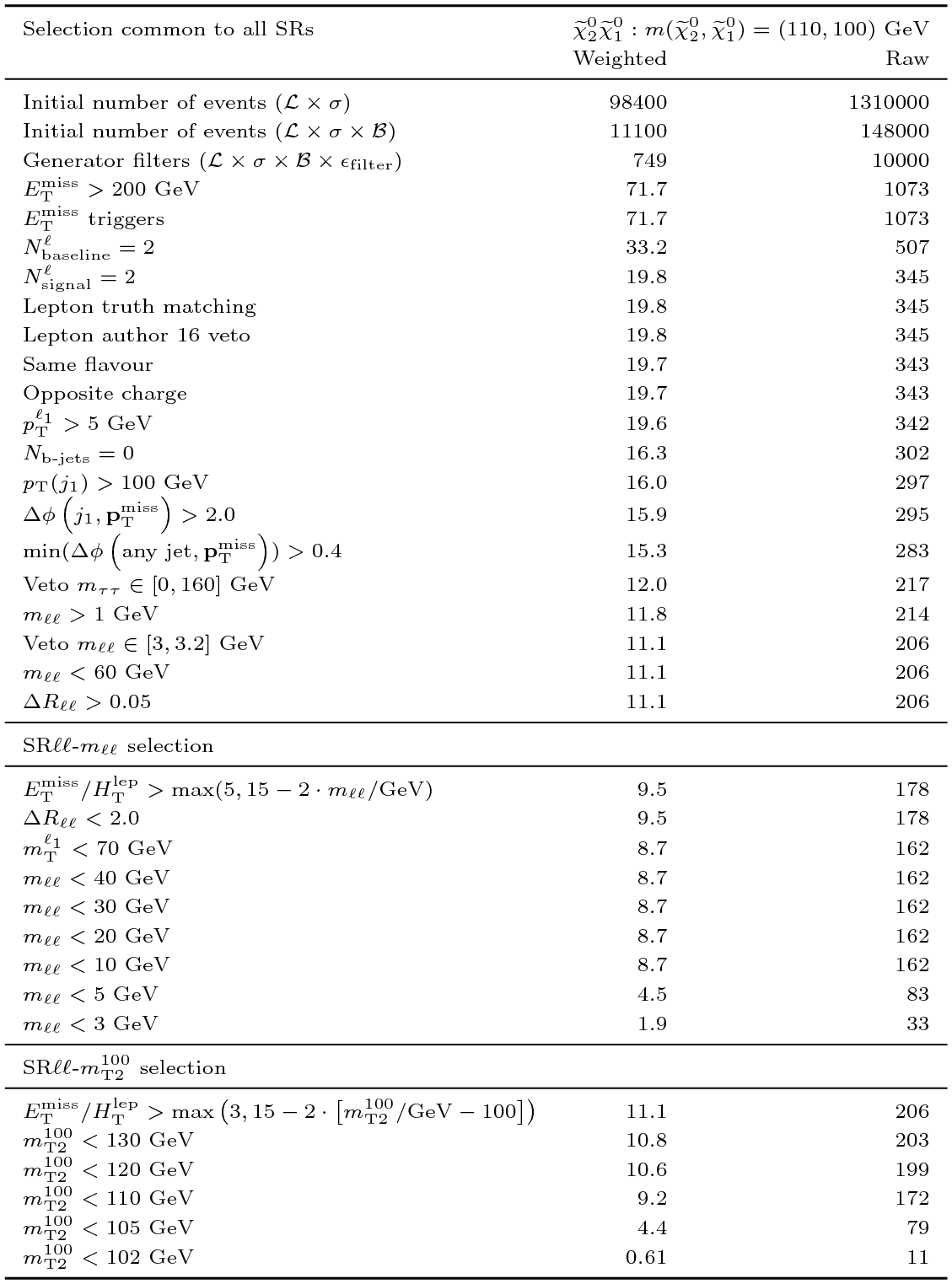
Table 12: Event counts for the χ̃₂⁰χ̃₁⁰ process of the Higgsino m(χ̃₂⁰, χ̃₁⁰) = (110, 100) GeV signal and sequentially with each addition requirement followed by those optimised for Higgsinos and sleptons. Weighted events are normalised to 36.1 fb^-1 and the raw Monte Carlo events are also displayed. png (44kB) pdf (71kB)
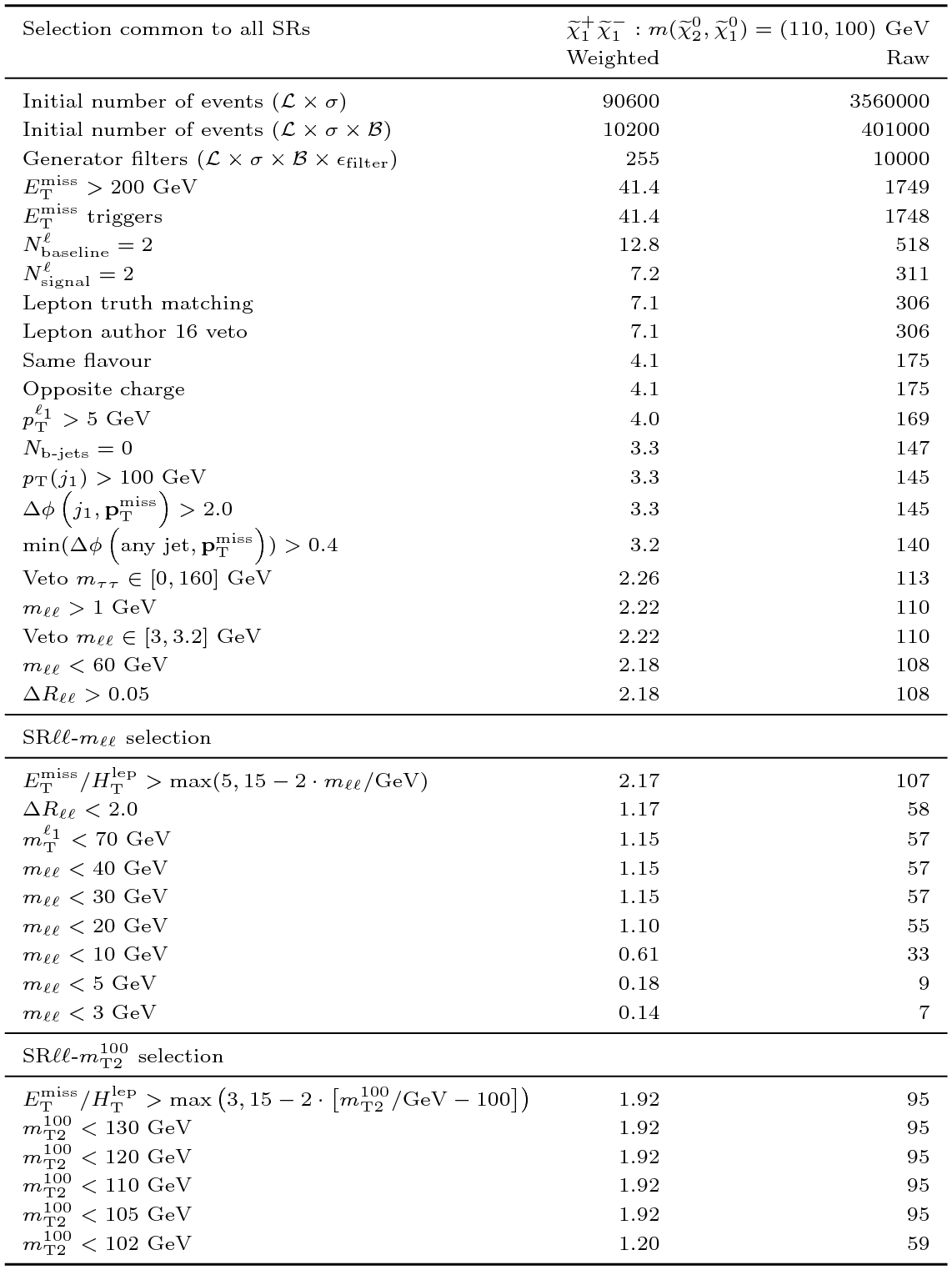
Table 13: Event counts for the χ̃₁⁺χ̃₁^- process of the Higgsino m(χ̃₂⁰, χ̃₁⁰) = (110, 100) GeV signal and sequentially with each addition requirement for selections common to all signal regions (SRs). ``Lepton truth matching" requires that the selected leptons are consistent with being decay products of the SUSY process. ``Lepton author 16 veto" removes a class of electron candidates reconstructed with algorithms designed to identify photon conversions. Weighted events are normalised to 36.1 fb^-1 and the raw Monte Carlo events are also displayed. png (42kB) pdf (78kB)

© 2017 CERN for the benefit of the ATLAS Collaboration. Reproduction of the article, figures and tables on this page is allowed as specified in the CC-BY-4.0 license.
2024-04-19 00:38:25