for
data presentation
February 15, 1996
Olivier Couet
CERN Geneva, Switzerland
Open Inventor is a high level graphics system build on top of OpenGL. It appears to be the next graphics standard for screen output.
Although, Open Inventor provides, a large number of high level graphics functionalities, some essential types of data representions, used in HEP, are not implemented in the basic standard.
This document describes in details all the various types of data represention used in HEP (mainly via the PAW system).
This document was initially written to provide the list of required features for the Open Inventor provider: TGS
The types of the objects presented graphically are: 1D histograms, 2D histograms, Ntuples, vectors and analytic functions.
For each type of representation and for each data type, a note is given according to the following rules:
![]()
![]()
![]() Essential, used very frequently.
Essential, used very frequently.
![]()
![]() Average usage
Average usage
![]() Seldom used.
Seldom used.
![]() Not used
Not used
Graphs are 2D representations of a set of points. The set of points can be defined by two vectors or by the content of an histogram: in that case the X coordinates are computed from the number of bins and the mininum and maximum X value.
The line graph is a simple polyline connecting the data set points. Axis and labels are computed from the data set itself and automatically drawn.
 |
1D histograms 2D histograms Ntuples Vectors Analytic functions |
|---|
Like the line graph the smooth curve connects the data set points. A B-spline interpolation is used to give a "smooth" representation of the curve. This type of represention is often used to display the result of a fit on a 1D histogram. Axis and labels are computed from the data set itself and automatically drawn.
 |
1D histograms 2D histograms Ntuples Vectors Analytic functions |
|---|
A marker is drawn at each point of the data set. The marker shape can be changed. This kind of representation is often used together with a line plot. Very often several data sets are drawn on the same plot. In this case, the marker type is used to identify the various data sets.
 |
1D histograms 2D histograms Ntuples Vectors Analytic functions |
|---|
This representation is the most frequently used for 1D histograms. For each bin, a vertical bar is drawn. The height of the bar is equal to the content of the bin. The width of the bar is less or equal to the width of the bin.
 |
1D histograms 2D histograms Ntuples Vectors Analytic functions |
|---|
Most of the physics results are presented with the error bars. The theoritical curve is drawn first and the experimental results are drawn on top with error bars. A data set may have up to 6 components when presented with error bars:
Very often, for each bin, the error on the X axis is equal to the bin width and the bottom and top error on the Y axis are equal.
This is the most common representation of error bars. Very often a marker is also drawn at each crossing point of the error bars.
 |
1D histograms 2D histograms Ntuples Vectors Analytic functions |
|---|
The addition of tick mark at the end of each bar gives a better idea where the bar stops. It may be useful when the curve hides partially the error bars.
 |
1D histograms 2D histograms Ntuples Vectors Analytic functions |
|---|
 |
1D histograms 2D histograms Ntuples Vectors Analytic functions |
|---|
 |
1D histograms 2D histograms Ntuples Vectors Analytic functions |
|---|
 |
1D histograms 2D histograms Ntuples Vectors Analytic functions |
|---|
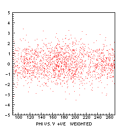
Each cell of the 2D data set is filled with a number of points proportional to the content of the cell.
 |
1D histograms 2D histograms Ntuples Vectors Analytic functions |
|---|
For each X,Y value of the Ntuple, a marker is drawn.
 |
1D histograms 2D histograms Ntuples Vectors Analytic functions |
|---|
Each cell of the 2D data set is filled with a box, of a surface proportional to the content of the cell.
 |
1D histograms 2D histograms Ntuples Vectors Analytic functions |
|---|
An arrow is drawn in each cell. The arrow size is proportional to the local slope an the arrow direction indicate the direction of the slope.
 |
1D histograms 2D histograms Ntuples Vectors Analytic functions |
|---|
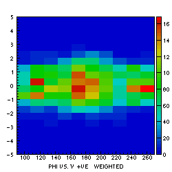
Each cell of the 2D data set is coloured according to a predefined colour map.
 |
1D histograms 2D histograms Ntuples Vectors Analytic functions |
|---|
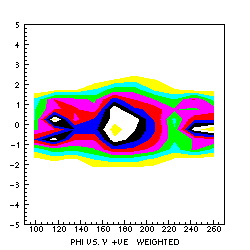
All the isovalues are connected with a line.
 |
1D histograms 2D histograms Ntuples Vectors Analytic functions |
|---|
Same as before, but the space between two isovalues is coloured.
 |
1D histograms 2D histograms Ntuples Vectors Analytic functions |
|---|
The contents of the each cell is simply printed.
 |
1D histograms 2D histograms Ntuples Vectors Analytic functions |
|---|
A character taken from a "character palette" is drawn in each cell.
 |
1D histograms 2D histograms Ntuples Vectors Analytic functions |
|---|
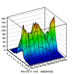
In this section are describe the 3D representation of 2D data set. In fact the kind of data sets are more 2D and a half because we have the two X and Y dimensions plus one and only one Z value for each (X,Y) pair. In case of histograms, the Z value is called ``bin content''.
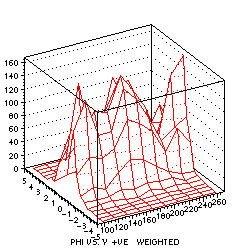
Each bin content is represented by a vertical 3D box. The hidden line removal technique allows to produce paper output on black and white printers (a hidden surface removal technique will produce a black picture on such printers).
 |
1D histograms 2D histograms Ntuples Vectors Analytic functions |
|---|
Each bin content is represented by a vertical 3D box. The hidden surface removal technique allows to produce coloured output.
 |
1D histograms 2D histograms Ntuples Vectors Analytic functions |
|---|
Each bin content is represented by a vertical 3D box. The hidden surface removal technique allows to produce coloured output. In this kind of representation, the bin content is also mapped on a colour map.
 |
1D histograms 2D histograms Ntuples Vectors Analytic functions |
|---|
 |
1D histograms 2D histograms Ntuples Vectors Analytic functions |
|---|
 |
1D histograms 2D histograms Ntuples Vectors Analytic functions |
|---|
 |
1D histograms 2D histograms Ntuples Vectors Analytic functions |
|---|
 |
1D histograms 2D histograms Ntuples Vectors Analytic functions |
|---|
 |
1D histograms 2D histograms Ntuples Vectors Analytic functions |
|---|
 |
1D histograms 2D histograms Ntuples Vectors Analytic functions |
|---|
 |
1D histograms 2D histograms Ntuples Vectors Analytic functions |
|---|
 |
1D histograms 2D histograms Ntuples Vectors Analytic functions |
|---|
 |
1D histograms 2D histograms Ntuples Vectors Analytic functions |
|---|
Various coordinate systems can be combined with the representation previously described:
Note that this kind of coordinate systems are available only on lego and surface in HIGZ. The polar coordinate system is also required in simple 2D plots.
 |
 |
 |
 |
|---|
Axis drawing is a very important feature for HEP. An axis drawing procedure should at least provide the following features:

