

Compact Muon Solenoid
LHC, CERN
| CMS-B2G-13-006 ; CERN-PH-EP-2015-170 | ||
| Search for pair-produced vectorlike B quarks in proton-proton collisions at $\sqrt{s} = $ 8 TeV | ||
| CMS Collaboration | ||
| 25 July 2015 | ||
| Phys. Rev. D 93 (2016) 112009 | ||
| Abstract: A search for the production of a heavy B quark, having electric charge -1/3 and vector couplings to W, Z, and H bosons, is carried out using proton-proton collision data recorded at the CERN LHC by the CMS experiment, corresponding to an integrated luminosity of 19.7 fb$^{-1}$. The B quark is assumed to be pair produced and to decay in one of three ways: to $\mathrm{ t }\mathrm{ W }$, $\mathrm{ b }\mathrm{ Z }$, or $\mathrm{ b }\mathrm{ H }$. The search is carried out in final states with one, two, and more than two charged leptons, as well as in fully hadronic final states. Each of the channels in the exclusive final-state topologies is designed to be sensitive to specific combinations of the B quark-antiquark pair decays. The observed event yields are found to be consistent with the standard model expectations in all the final states studied. A statistical combination of these results is performed, and upper limits are set on the cross section of the strongly produced B quark-antiquark pairs as a function of the B quark mass. Lower limits on the B quark mass between 740 and 900 GeV are set at a 95% confidence level, depending on the values of the branching fractions of the B quark to $\mathrm{ t }\mathrm{ W }$, $\mathrm{ b }\mathrm{ Z }$, and $\mathrm{ b }\mathrm{ H }$. Overall, these limits are the most stringent to date. | ||
| Links: e-print arXiv:1507.07129 [hep-ex] (PDF) ; CDS record ; inSPIRE record ; HepData record ; CADI line (restricted) ; | ||
| Figures | |
png pdf |
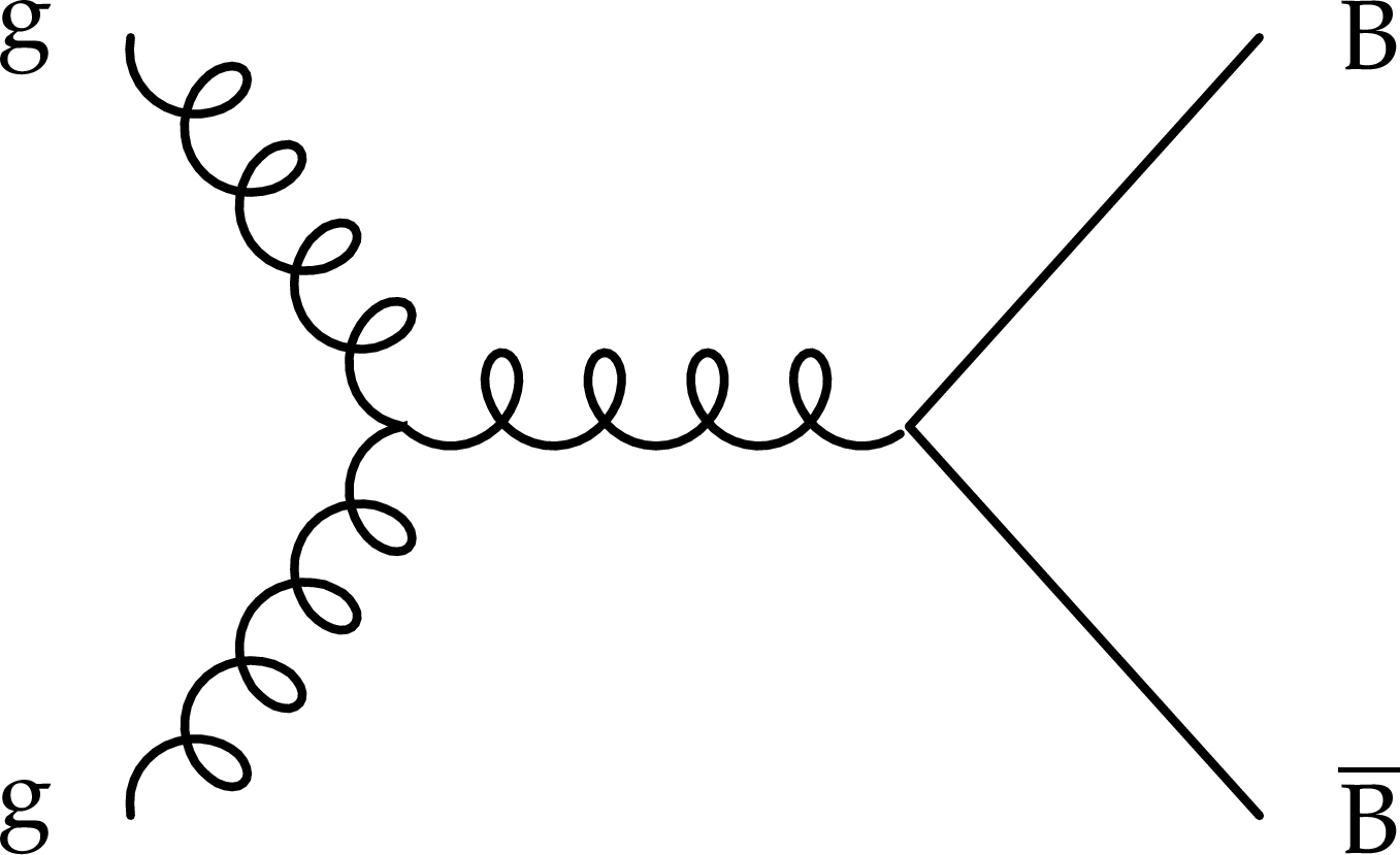
Figure 1-a:
Feynman diagrams for the dominant B quark pair-production process (top) and for the B quark decay modes (bottom). |
png pdf |
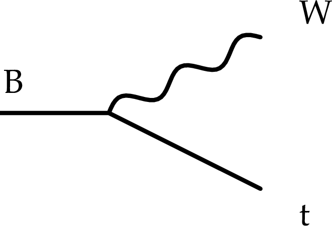
Figure 1-b:
Feynman diagrams for the dominant B quark pair-production process (top) and for the B quark decay modes (bottom). |
png pdf |
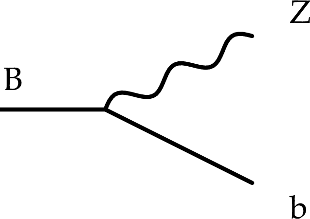
Figure 1-c:
Feynman diagrams for the dominant B quark pair-production process (top) and for the B quark decay modes (bottom). |
png pdf |
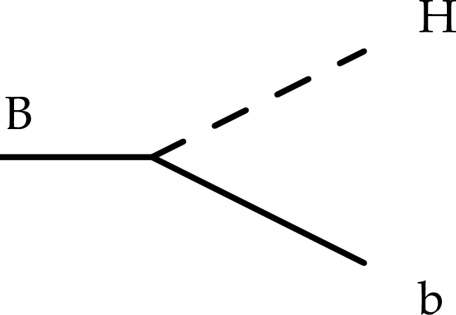
Figure 1-d:
Feynman diagrams for the dominant B quark pair-production process (top) and for the B quark decay modes (bottom). |
png pdf |
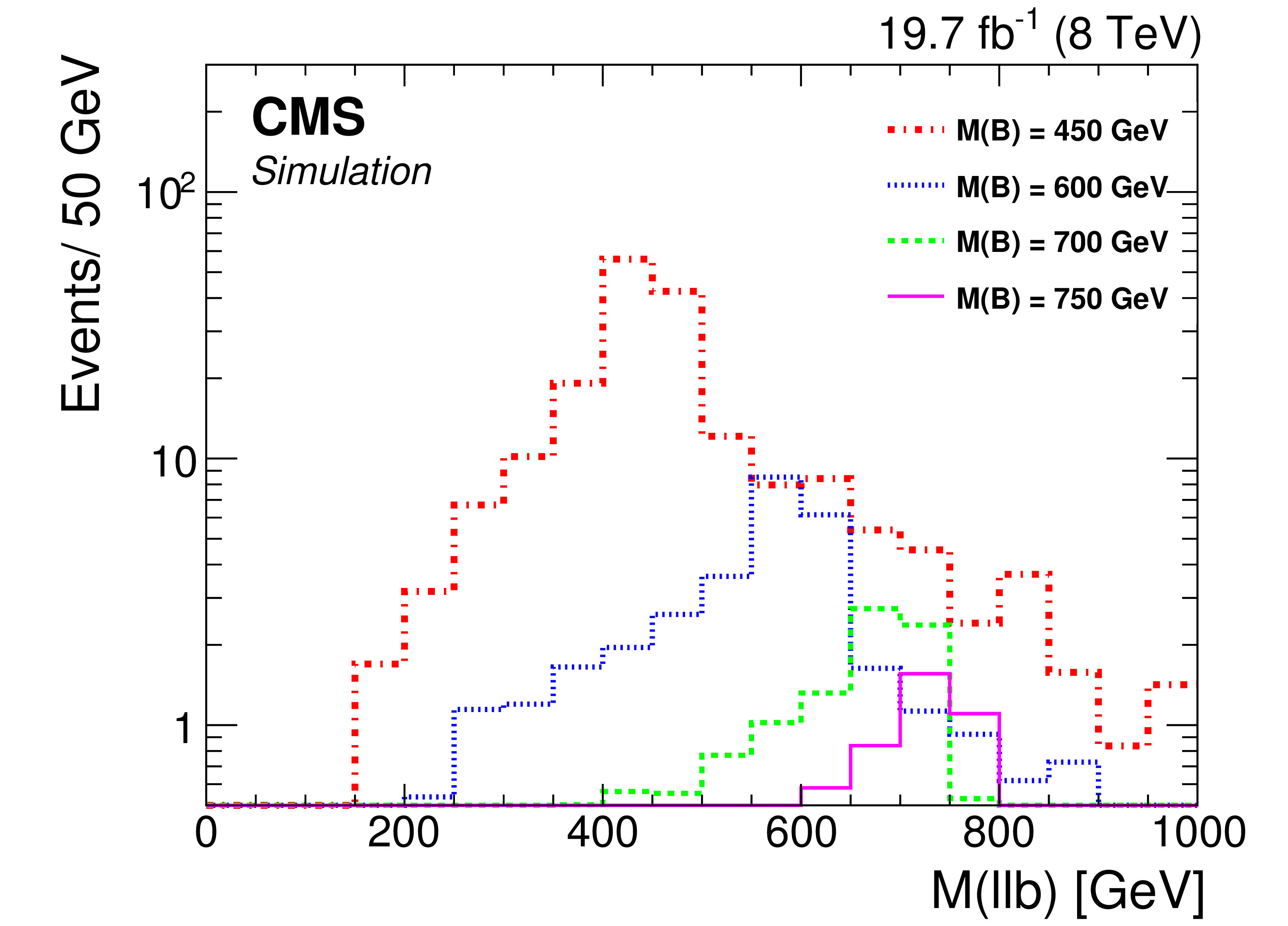
Figure 2:
The reconstructed mass of the B quark candidate in the opposite-sign lepton pair channel, using the invariant mass of the dilepton and b-jet in simulated events. |
png pdf |
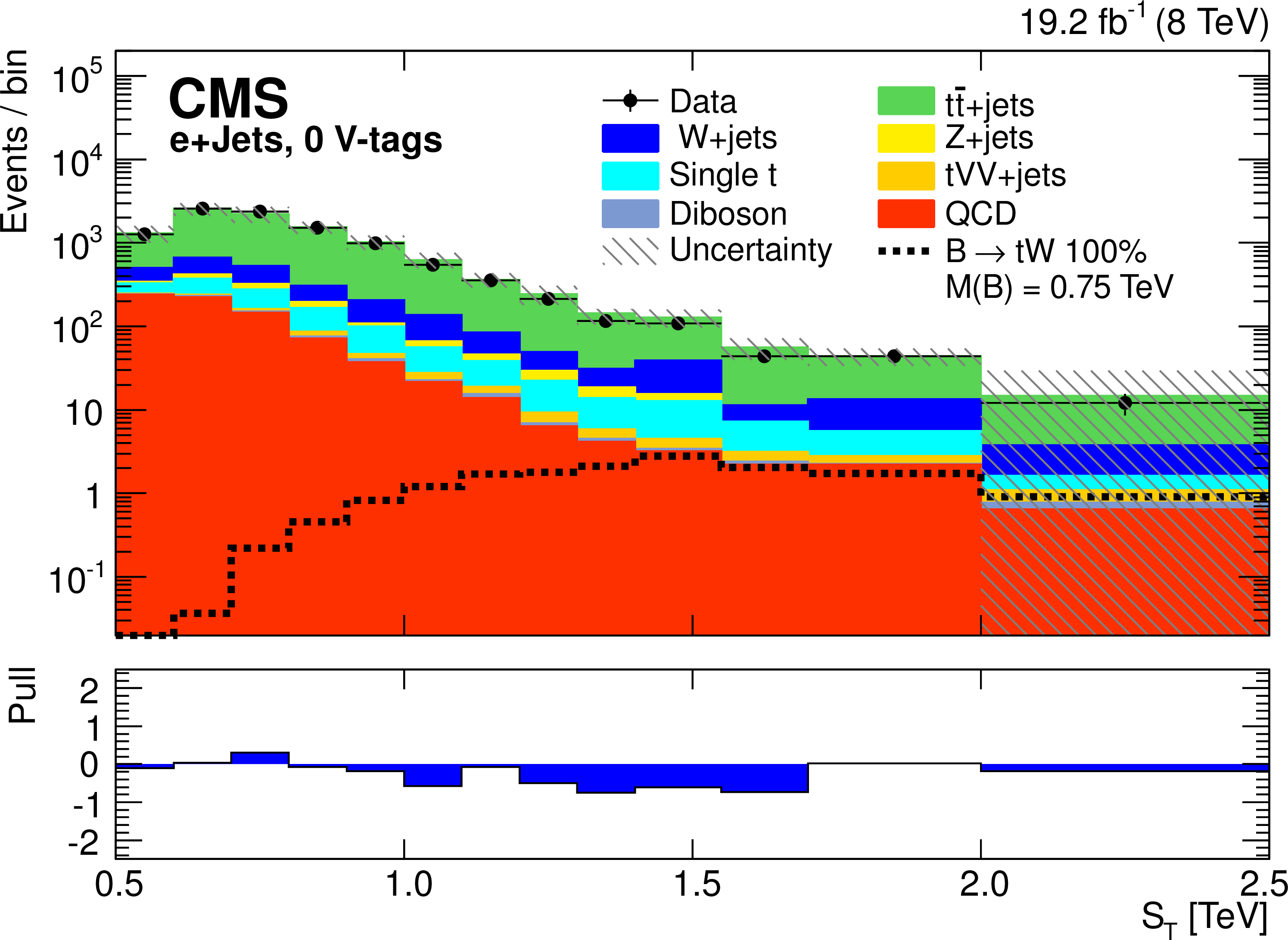
Figure 3-a:
The $ {S_{\mathrm {T}}} $ distributions in the 0, 1, and ${\geq} $2 V-tag categories in the electron+jets channel (a,c,e) and muon+jets channel (b,d,f). The uncertainty bands shown include statistical and all systematic uncertainties, added in quadrature for each single bin. The horizontal bars on the data points indicate the bin width. The difference between the observed and expected events divided by the total statistical and systematic uncertainty of the background prediction (pull) is shown for each bin in the lower panels. |
png pdf |
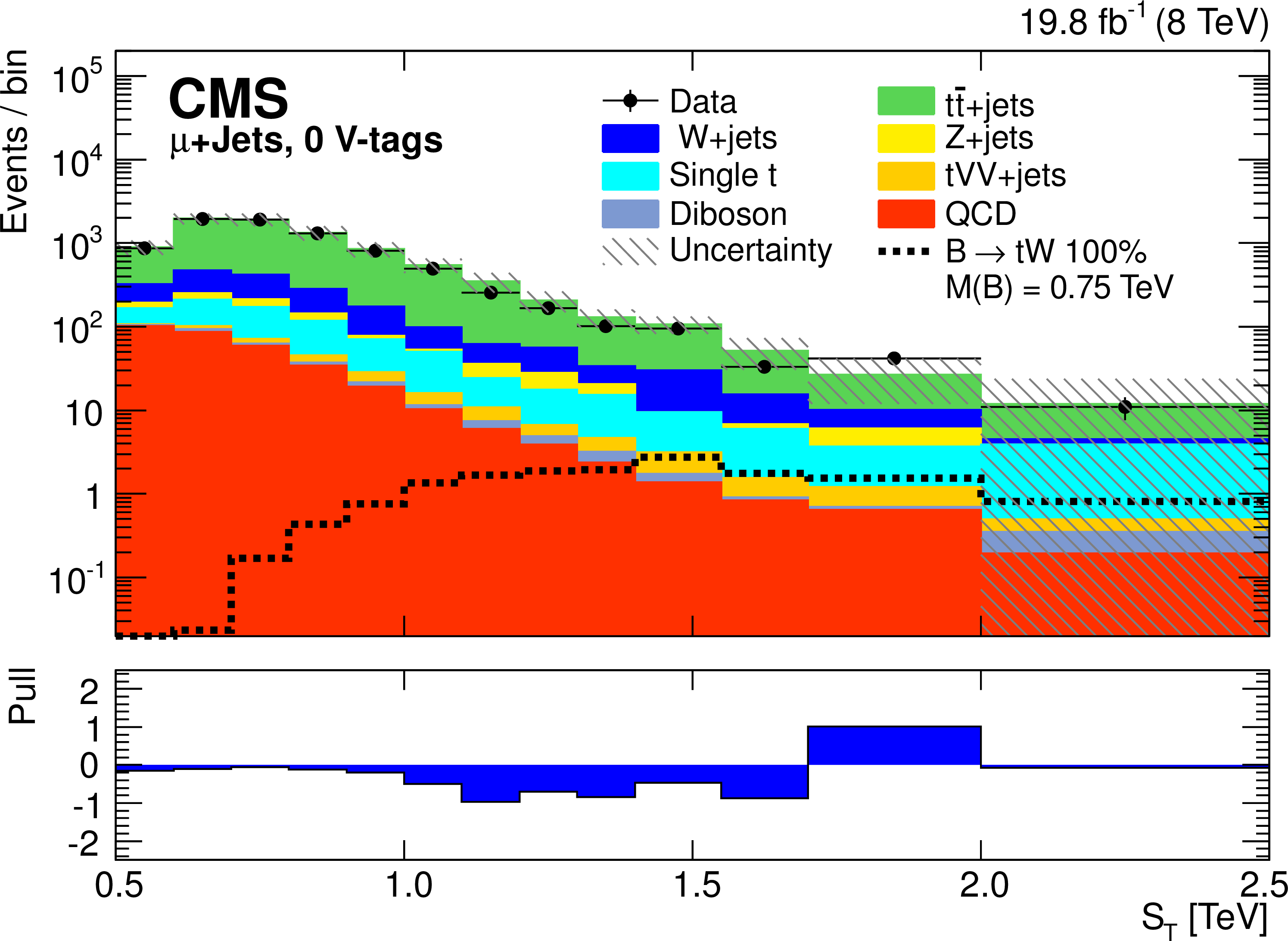
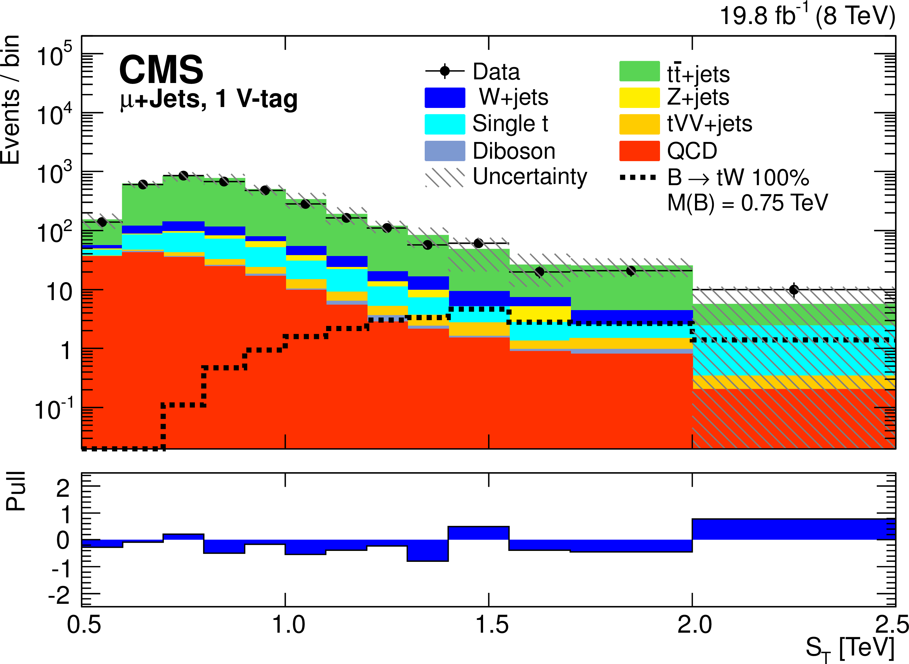
Figure 3-b:
The $ {S_{\mathrm {T}}} $ distributions in the 0, 1, and ${\geq} $2 V-tag categories in the electron+jets channel (a,c,e) and muon+jets channel (b,d,f). The uncertainty bands shown include statistical and all systematic uncertainties, added in quadrature for each single bin. The horizontal bars on the data points indicate the bin width. The difference between the observed and expected events divided by the total statistical and systematic uncertainty of the background prediction (pull) is shown for each bin in the lower panels. |
png pdf |
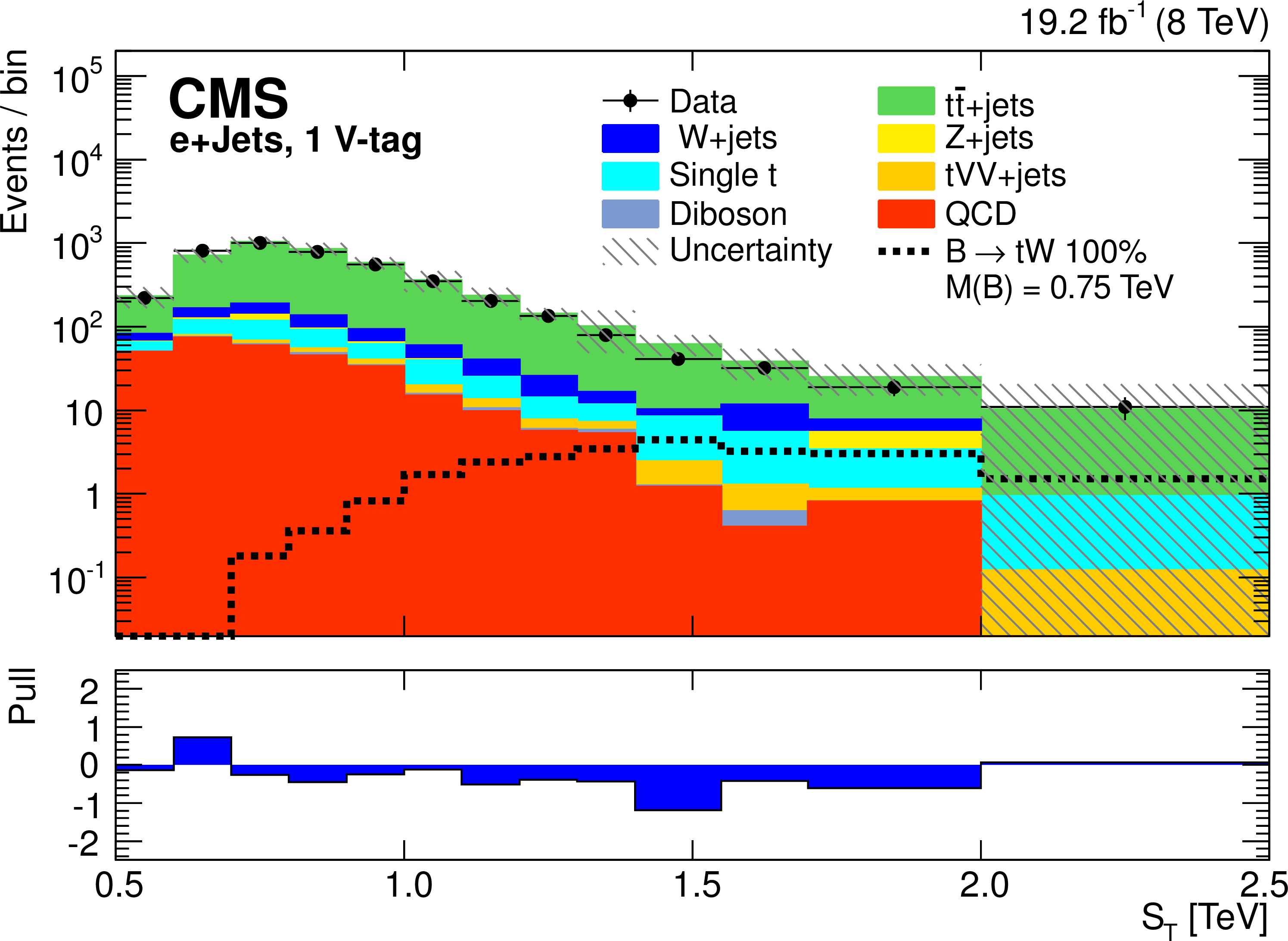
Figure 3-c:
The $ {S_{\mathrm {T}}} $ distributions in the 0, 1, and ${\geq} $2 V-tag categories in the electron+jets channel (a,c,e) and muon+jets channel (b,d,f). The uncertainty bands shown include statistical and all systematic uncertainties, added in quadrature for each single bin. The horizontal bars on the data points indicate the bin width. The difference between the observed and expected events divided by the total statistical and systematic uncertainty of the background prediction (pull) is shown for each bin in the lower panels. |
png pdf |
Figure 3-d:
The $ {S_{\mathrm {T}}} $ distributions in the 0, 1, and ${\geq} $2 V-tag categories in the electron+jets channel (a,c,e) and muon+jets channel (b,d,f). The uncertainty bands shown include statistical and all systematic uncertainties, added in quadrature for each single bin. The horizontal bars on the data points indicate the bin width. The difference between the observed and expected events divided by the total statistical and systematic uncertainty of the background prediction (pull) is shown for each bin in the lower panels. |
png pdf |
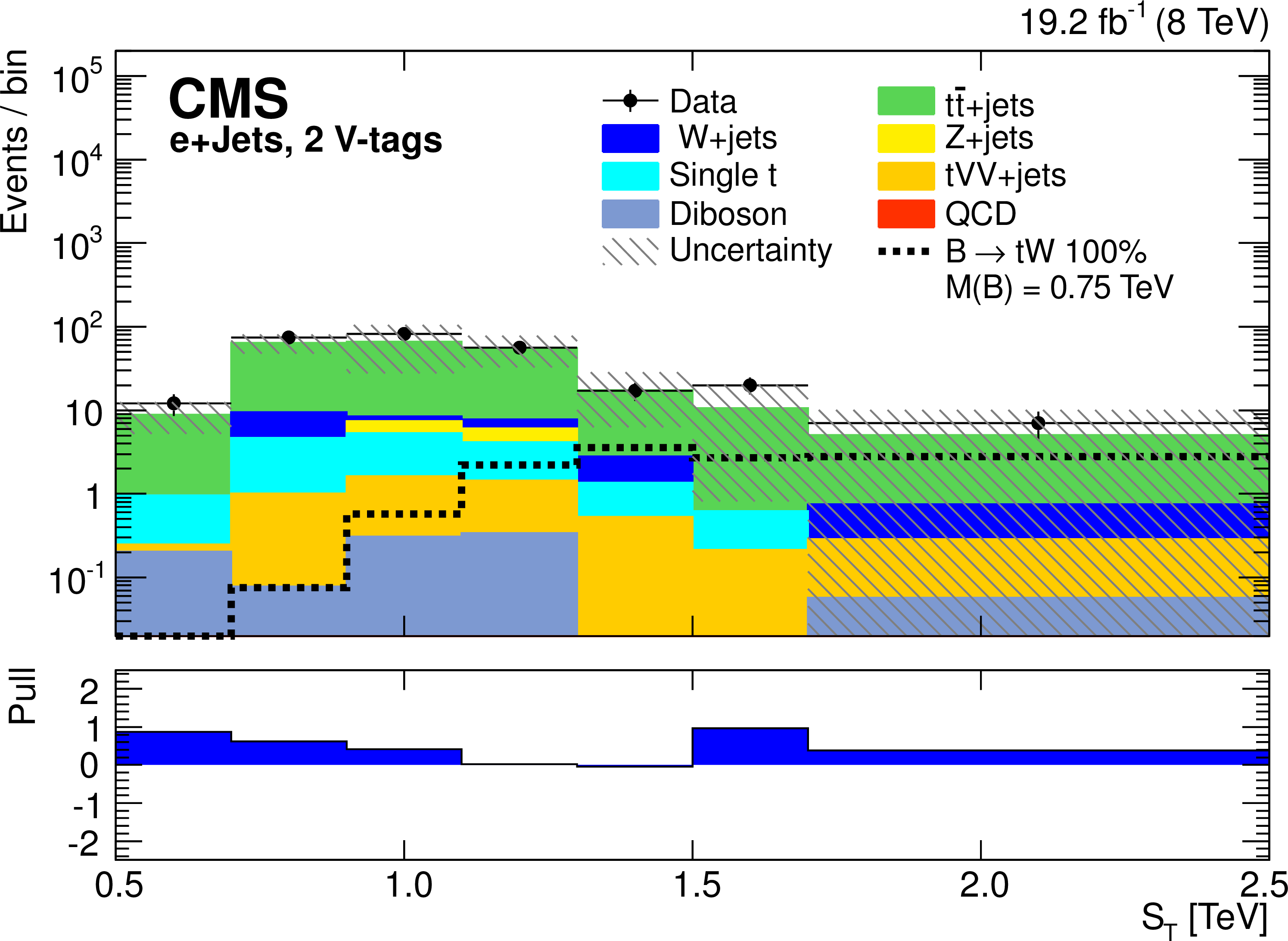
Figure 3-e:
The $ {S_{\mathrm {T}}} $ distributions in the 0, 1, and ${\geq} $2 V-tag categories in the electron+jets channel (a,c,e) and muon+jets channel (b,d,f). The uncertainty bands shown include statistical and all systematic uncertainties, added in quadrature for each single bin. The horizontal bars on the data points indicate the bin width. The difference between the observed and expected events divided by the total statistical and systematic uncertainty of the background prediction (pull) is shown for each bin in the lower panels. |
png pdf |
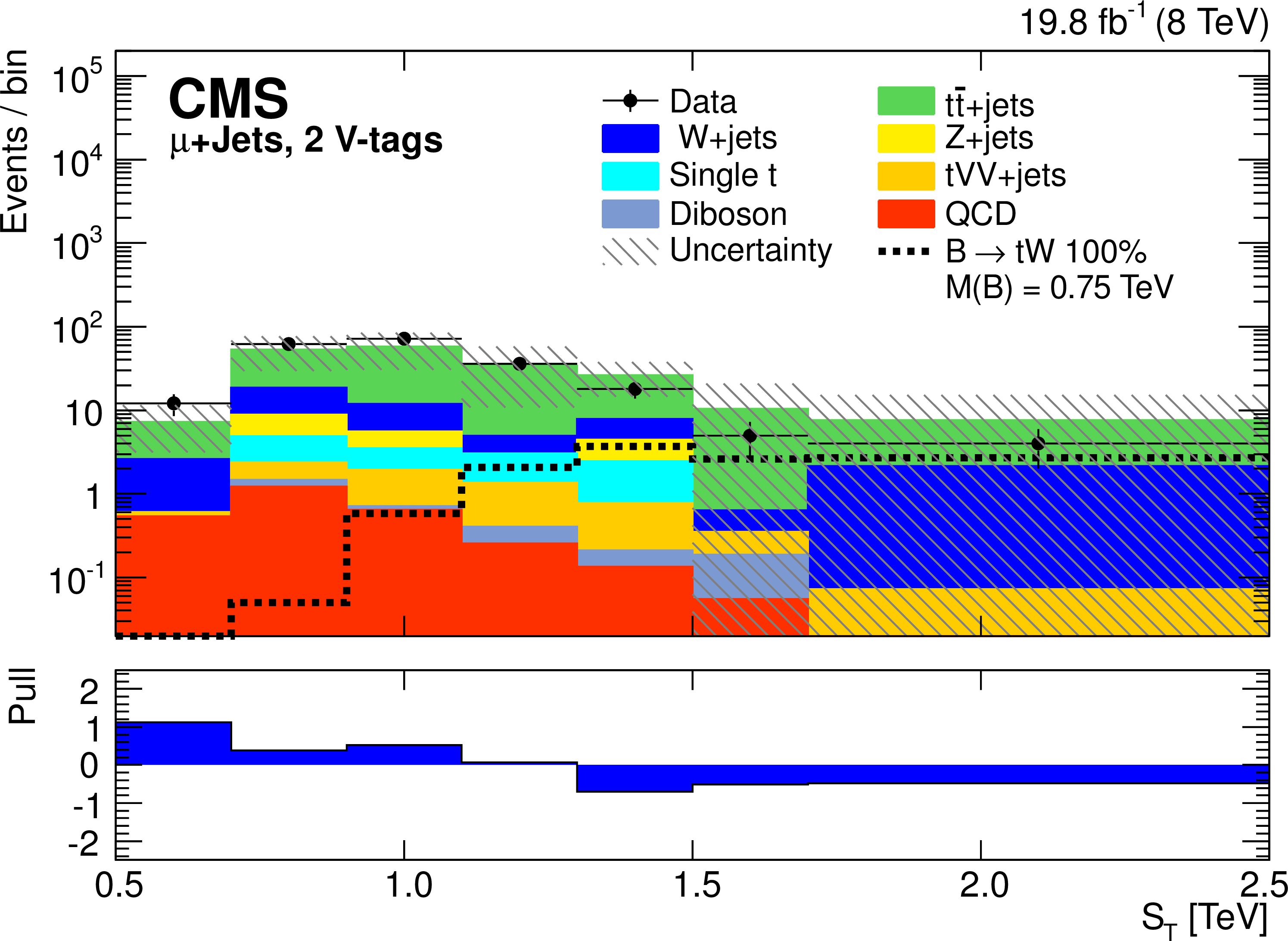
Figure 3-f:
The $ {S_{\mathrm {T}}} $ distributions in the 0, 1, and ${\geq} $2 V-tag categories in the electron+jets channel (a,c,e) and muon+jets channel (b,d,f). The uncertainty bands shown include statistical and all systematic uncertainties, added in quadrature for each single bin. The horizontal bars on the data points indicate the bin width. The difference between the observed and expected events divided by the total statistical and systematic uncertainty of the background prediction (pull) is shown for each bin in the lower panels. |
png pdf |
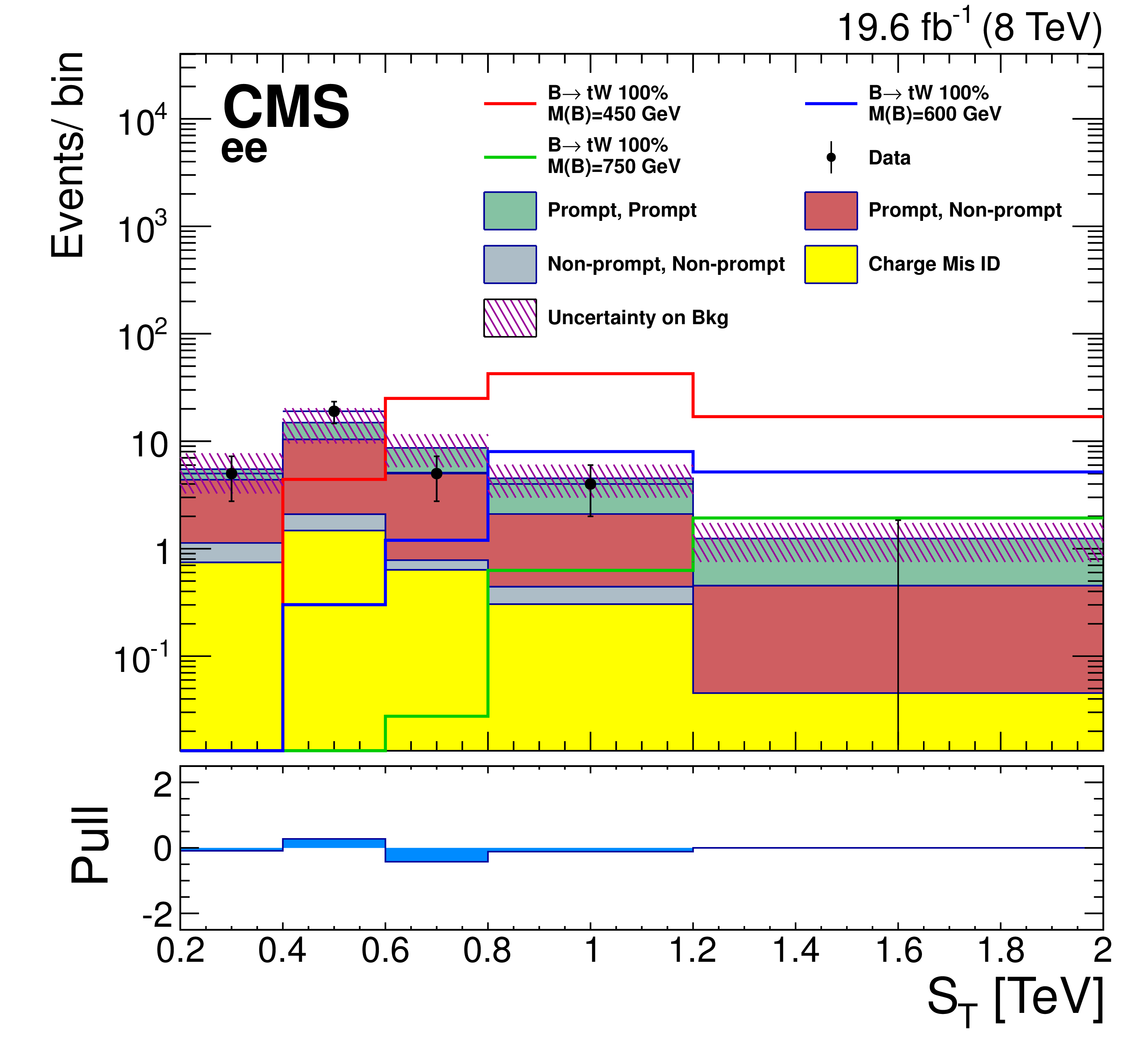
Figure 4-a:
The ${S_{\mathrm {T}}}$ distributions used for signal discrimination in the same-sign dilepton channel. The distribution is shown for the three dilepton categories used: dielectron (a), dimuon (b), and electron-muon (c). The horizontal bars on the data points indicate the bin width. The difference between the observed and expected events divided by the total statistical and systematic uncertainty of the background prediction (pull) is shown for each bin in the lower panels. |
png pdf |
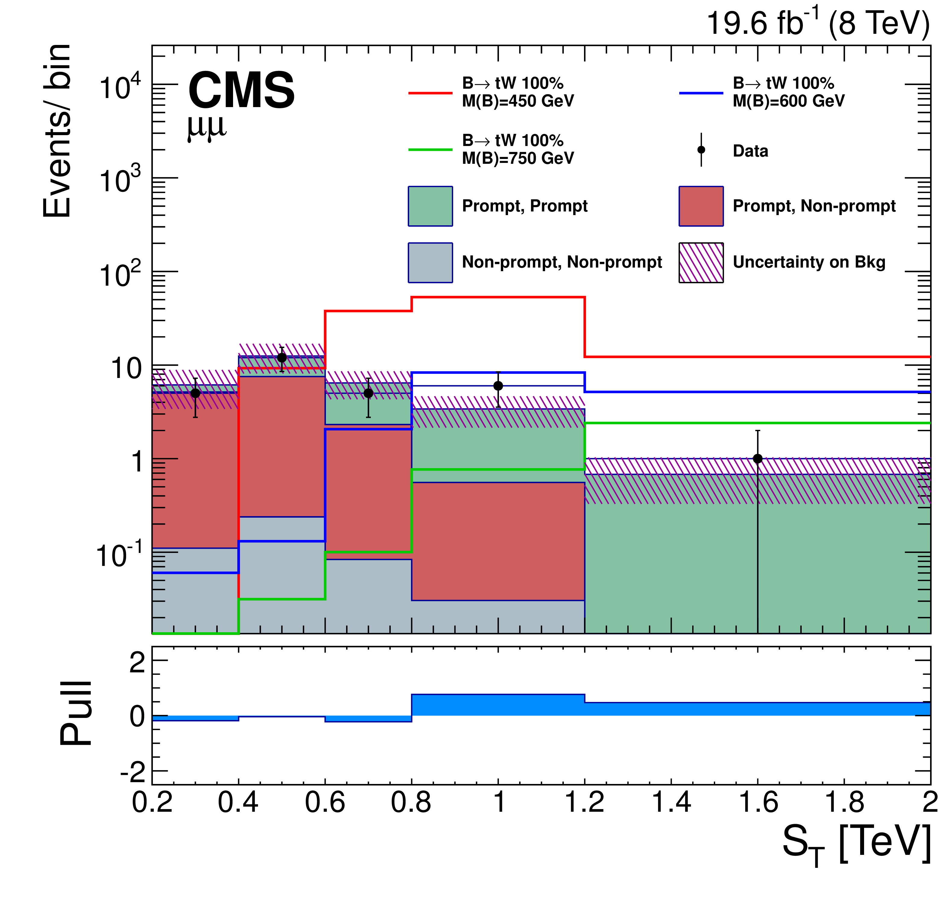
Figure 4-b:
The ${S_{\mathrm {T}}}$ distributions used for signal discrimination in the same-sign dilepton channel. The distribution is shown for the three dilepton categories used: dielectron (a), dimuon (b), and electron-muon (c). The horizontal bars on the data points indicate the bin width. The difference between the observed and expected events divided by the total statistical and systematic uncertainty of the background prediction (pull) is shown for each bin in the lower panels. |

png pdf |
Figure 4-c:
The ${S_{\mathrm {T}}}$ distributions used for signal discrimination in the same-sign dilepton channel. The distribution is shown for the three dilepton categories used: dielectron (a), dimuon (b), and electron-muon (c). The horizontal bars on the data points indicate the bin width. The difference between the observed and expected events divided by the total statistical and systematic uncertainty of the background prediction (pull) is shown for each bin in the lower panels. |

png pdf |
Figure 5-a:
The event distribution in the plane of $N_\text {jets}$ vs the b-tagging discriminator value, used to define the regions $A$, $B$, $C$, and $D$ for the opposite-sign dilepton ${{\mathrm{ Z } } \to \mathrm{ e }^- \mathrm{ e }^+ }$ (a) and ${{\mathrm{ Z } } \to \mu^+ \mu^- }$ (b) channels. The region $B$ is the signal region while the others constitute the control regions. The regions $I$, $J$, $K$, and $L$ are used for estimation of systematic uncertainties. All other selection criteria used to select the B quark candidates have been applied. The area of each bar is proportional to the number of events in a given bin of the distribution of $N_\text {jets}$ vs b-tagging discriminator. |
png pdf |
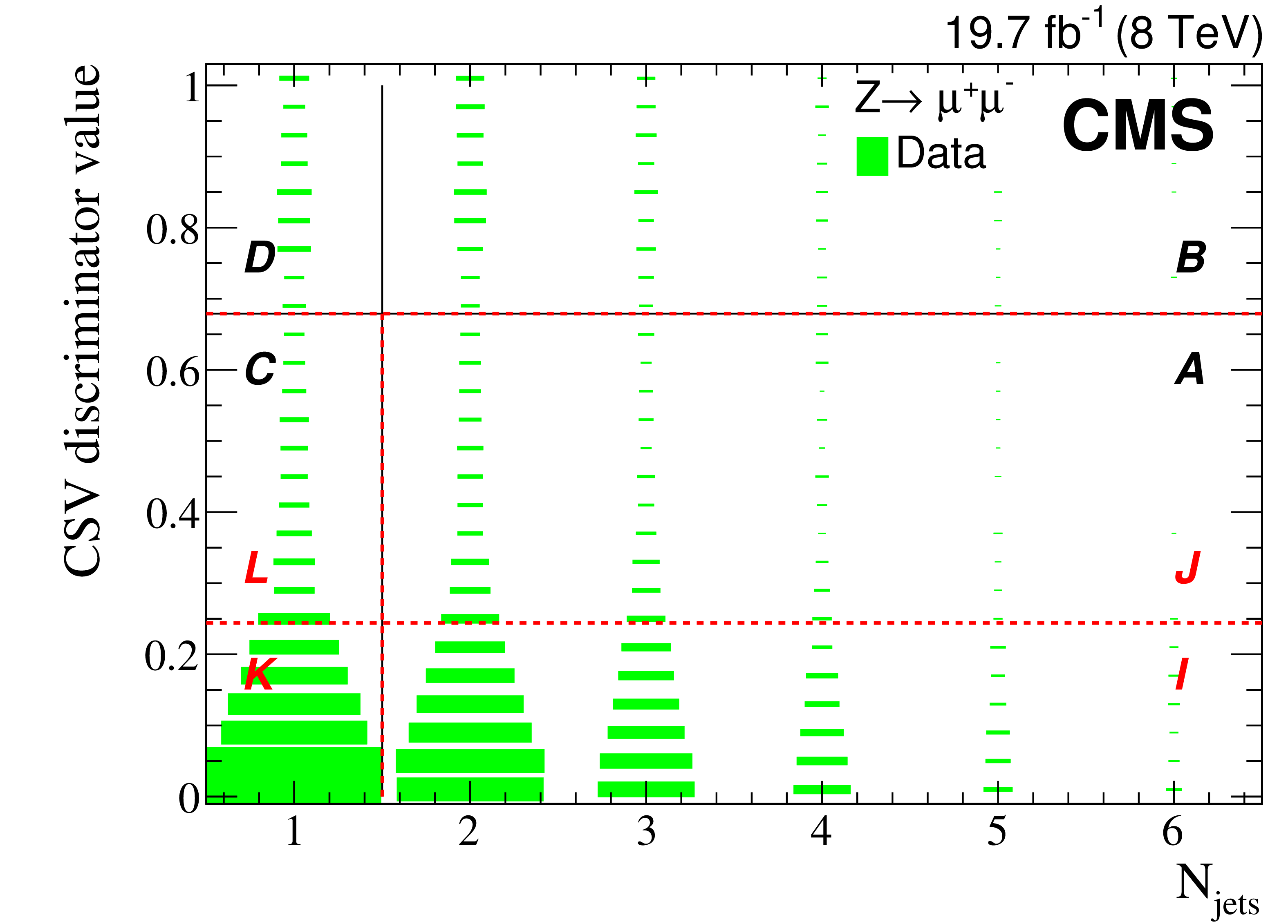
Figure 5-b:
The event distribution in the plane of $N_\text {jets}$ vs the b-tagging discriminator value, used to define the regions $A$, $B$, $C$, and $D$ for the opposite-sign dilepton ${{\mathrm{ Z } } \to \mathrm{ e }^- \mathrm{ e }^+ }$ (a) and ${{\mathrm{ Z } } \to \mu^+ \mu^- }$ (b) channels. The region $B$ is the signal region while the others constitute the control regions. The regions $I$, $J$, $K$, and $L$ are used for estimation of systematic uncertainties. All other selection criteria used to select the B quark candidates have been applied. The area of each bar is proportional to the number of events in a given bin of the distribution of $N_\text {jets}$ vs b-tagging discriminator. |
png pdf |
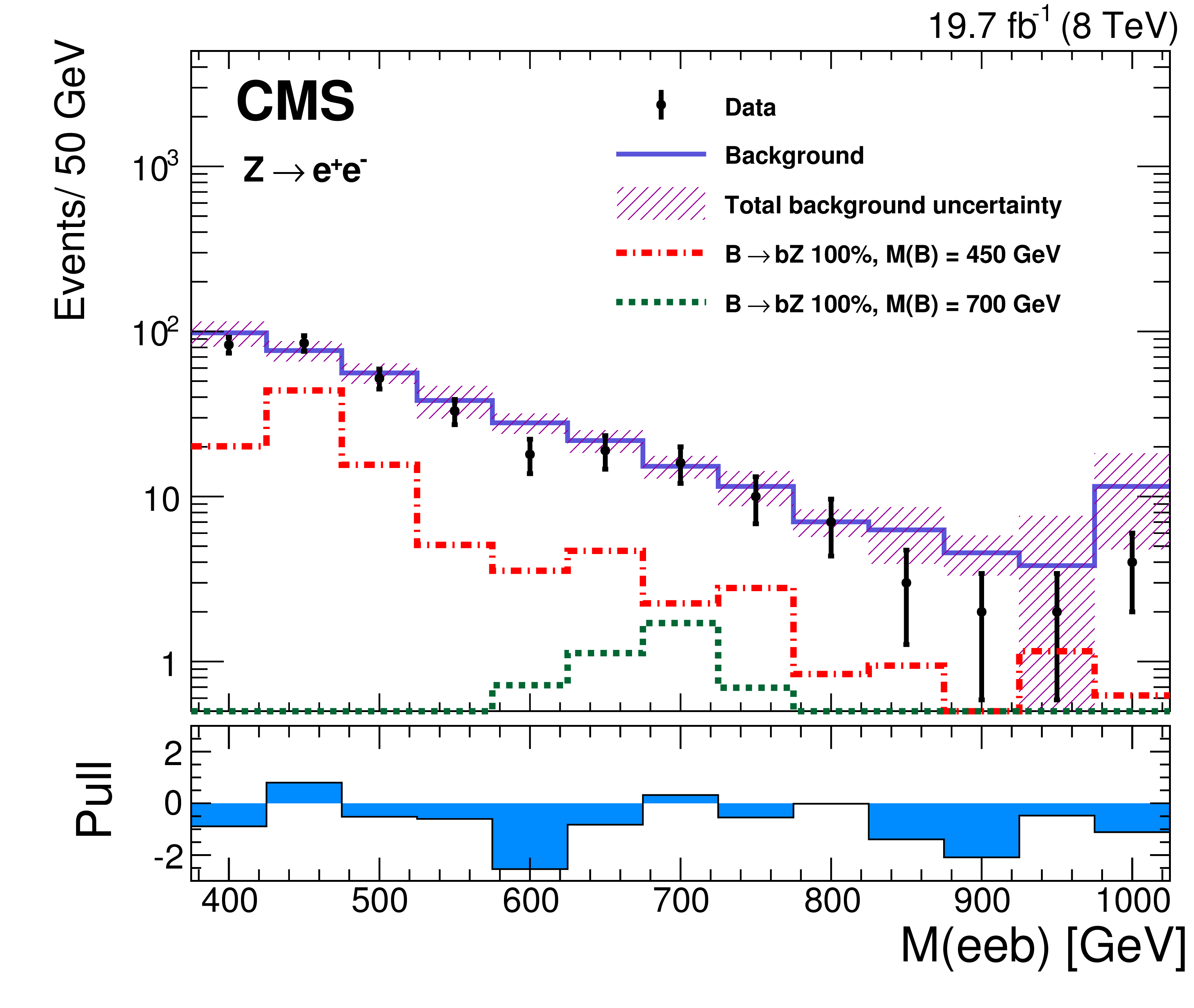
Figure 6-a:
The invariant mass of reconstructed B quark candidates in the opposite-sign dilepton ${{\mathrm{ Z } } \to \mathrm{ e }^- \mathrm{ e }^+ }$ (a) and ${{\mathrm{ Z } } \to \mu^+ \mu^- } $ (b) channels. The estimated background is shown by the solid line, along with the total uncertainty (hatched area). The last bin of the histograms contains all events with $ {M(\ell \ell \mathrm{ b } )} > $ 1000 GeV. The signal contribution is shown for two B quark masses. The difference between the observed and expected events divided by the total statistical and systematic uncertainty of the background prediction (pull) is shown for each bin in the lower panels. |
png pdf |
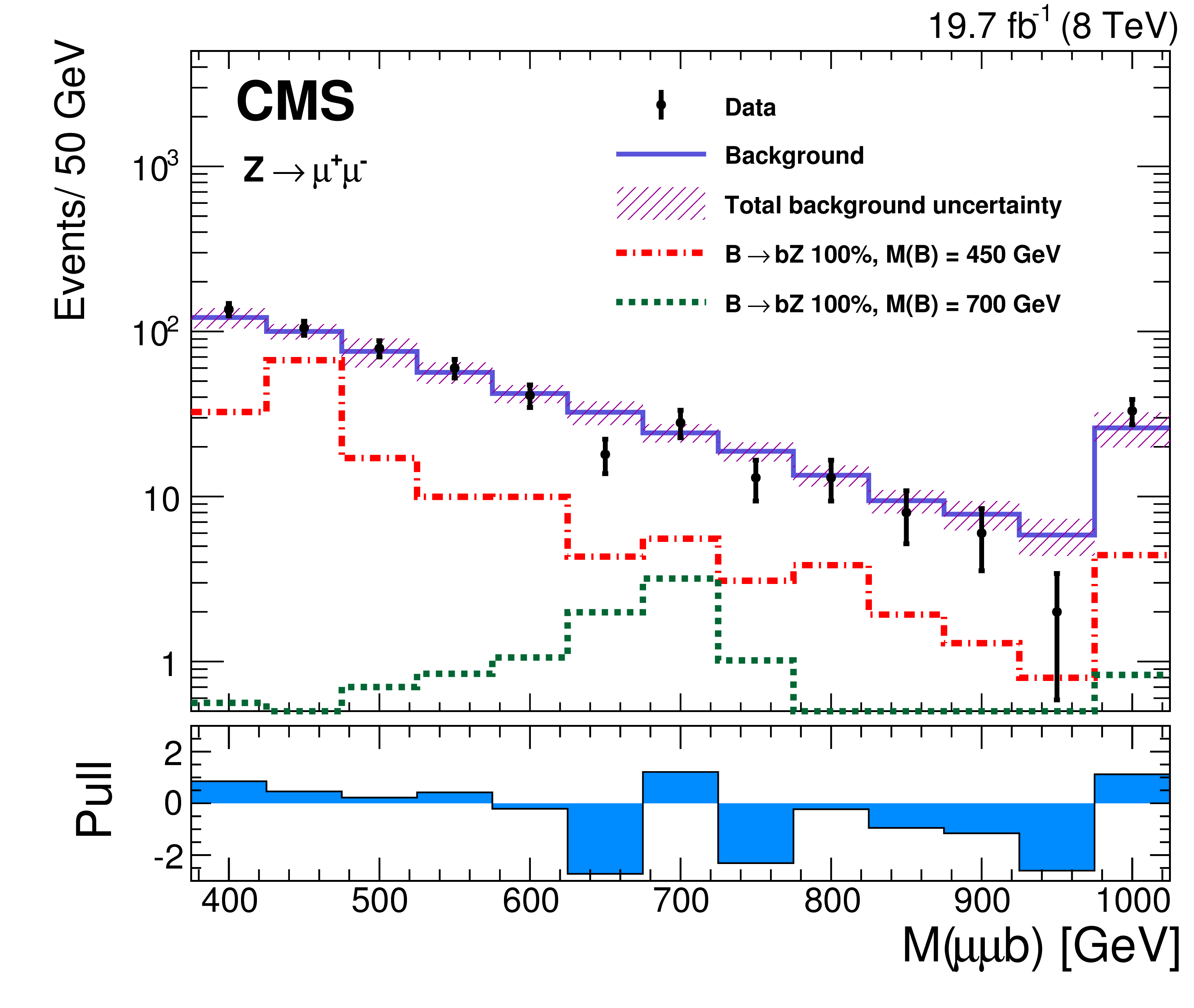
Figure 6-b:
The invariant mass of reconstructed B quark candidates in the opposite-sign dilepton ${{\mathrm{ Z } } \to \mathrm{ e }^- \mathrm{ e }^+ }$ (a) and ${{\mathrm{ Z } } \to \mu^+ \mu^- } $ (b) channels. The estimated background is shown by the solid line, along with the total uncertainty (hatched area). The last bin of the histograms contains all events with $ {M(\ell \ell \mathrm{ b } )} > $ 1000 GeV. The signal contribution is shown for two B quark masses. The difference between the observed and expected events divided by the total statistical and systematic uncertainty of the background prediction (pull) is shown for each bin in the lower panels. |
png pdf |
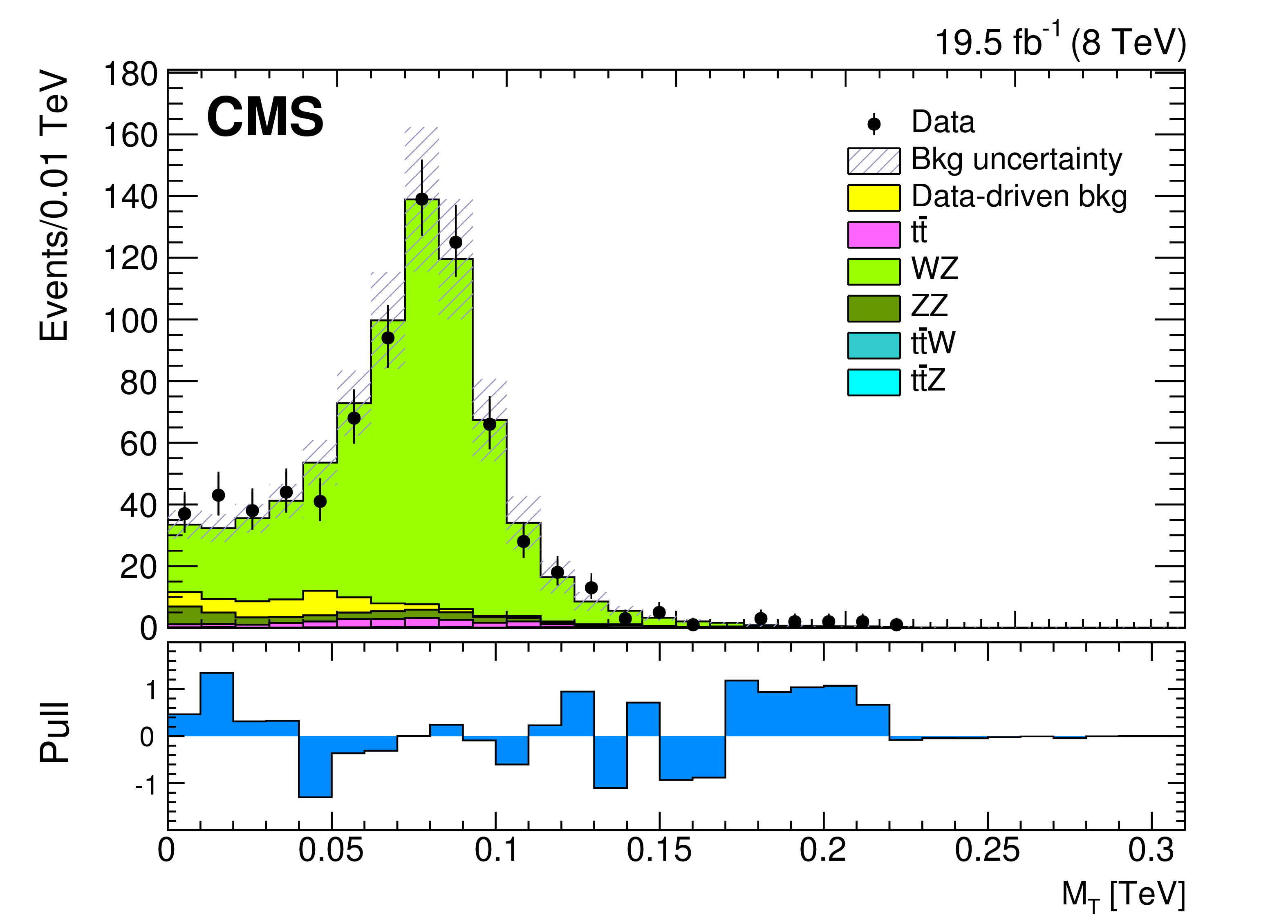
Figure 7-a:
The transverse mass $M_{\mathrm{T}}$ distribution of events in a control sample of the multilepton analysis, enriched in $\mathrm{ W } {\mathrm{ Z } } $ by requiring an OSSF pair with $M(\ell \ell )$ in the Z boson mass window and 50 $ < {E_{\mathrm {T}}} < $ 100 GeV (a). The ${S_{\mathrm {T}}}$ distribution for events containing an opposite-sign $\mathrm{ e } \mu $ pair in the ${\mathrm{ t \bar{t} } }$ control region of the multilepton analysis (b). Uncertainties include both statistical and systematic contributions. The difference between the observed and expected events divided by the total statistical and systematic uncertainty of the background prediction (pull) is shown for each bin in the lower panels. |
png pdf |
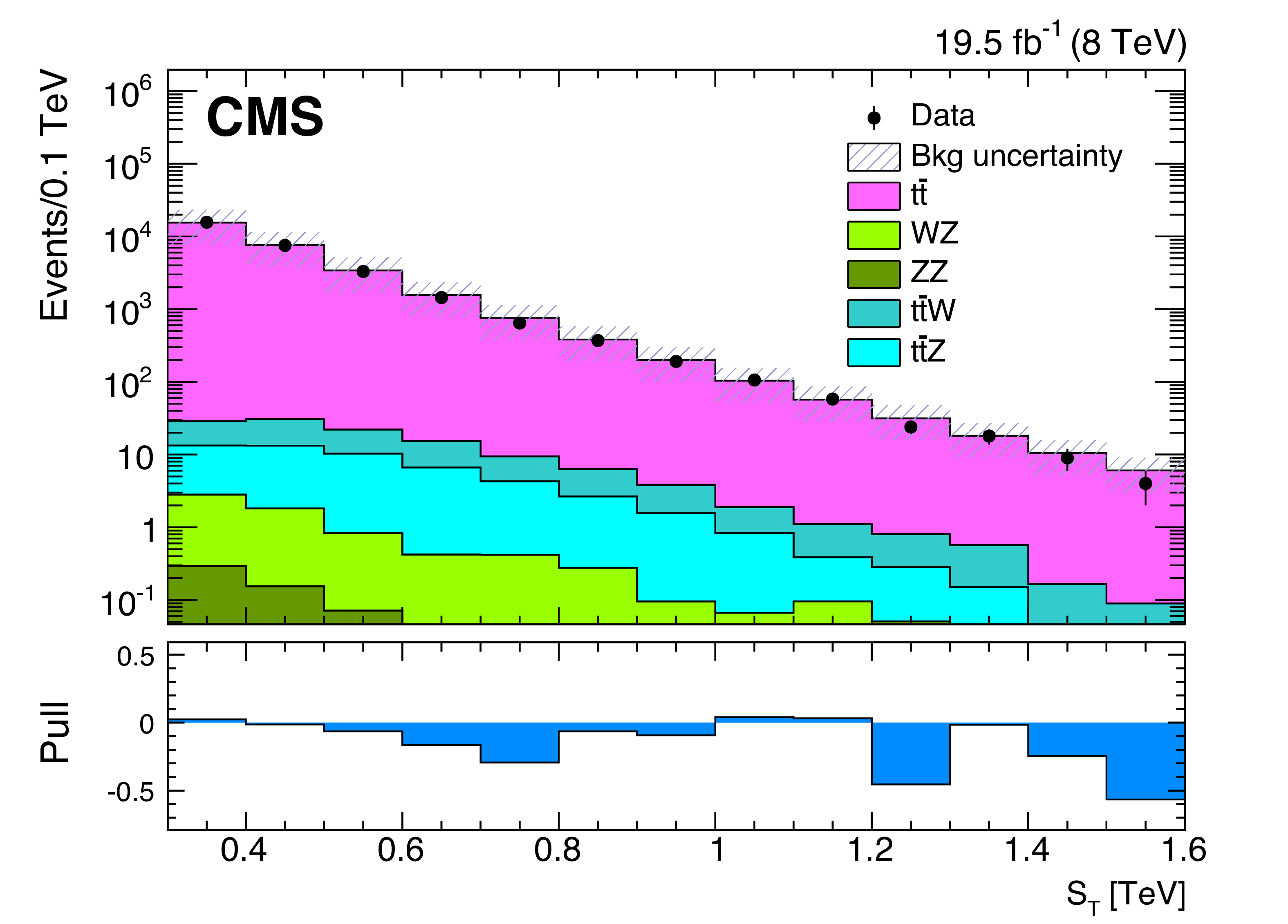
Figure 7-b:
The transverse mass $M_{\mathrm{T}}$ distribution of events in a control sample of the multilepton analysis, enriched in $\mathrm{ W } {\mathrm{ Z } } $ by requiring an OSSF pair with $M(\ell \ell )$ in the Z boson mass window and 50 $ < {E_{\mathrm {T}}} < $ 100 GeV (a). The ${S_{\mathrm {T}}}$ distribution for events containing an opposite-sign $\mathrm{ e } \mu $ pair in the ${\mathrm{ t \bar{t} } }$ control region of the multilepton analysis (b). Uncertainties include both statistical and systematic contributions. The difference between the observed and expected events divided by the total statistical and systematic uncertainty of the background prediction (pull) is shown for each bin in the lower panels. |
png pdf |
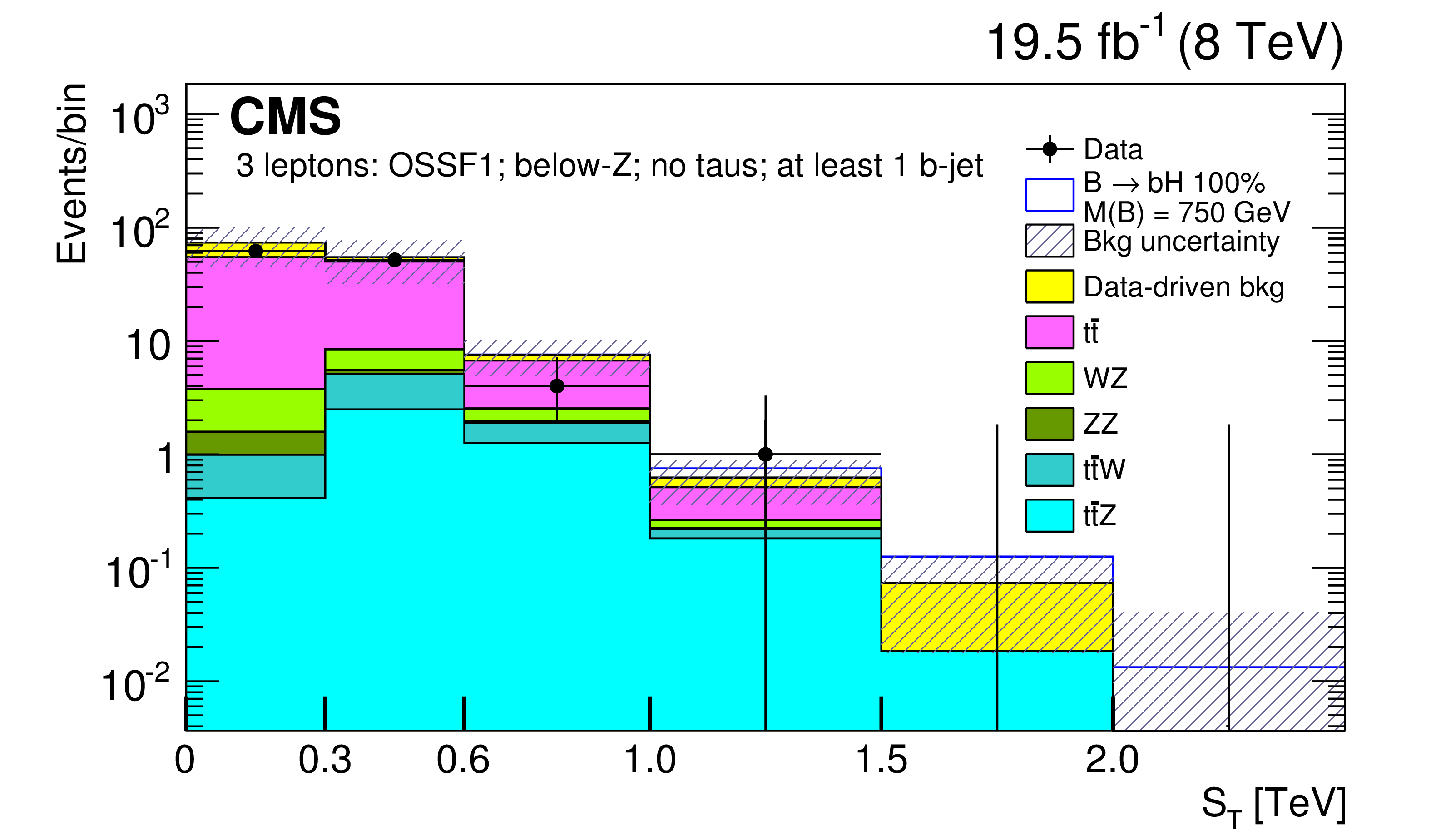
Figure 8-a:
Distributions of ${S_{\mathrm {T}}}$ for two event categorizations in the multilepton channel: (a) three leptons, no tau leptons, at least one b-tagged jet, and no reconstructed Z boson candidate; (b) four leptons, one tau lepton, no b-tagged jets, and one reconstructed Z boson candidate. Uncertainties include both statistical and systematic contributions. The data-driven contribution includes contributions from two genuine leptons and one or more misidentified leptons. The horizontal bars on the data points indicate the bin width. |
png pdf |
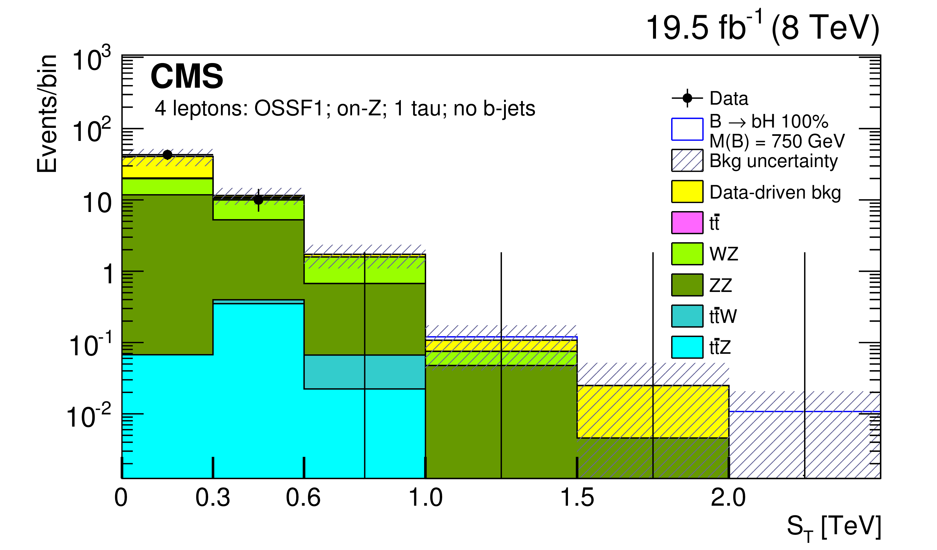
Figure 8-b:
Distributions of ${S_{\mathrm {T}}}$ for two event categorizations in the multilepton channel: (a) three leptons, no tau leptons, at least one b-tagged jet, and no reconstructed Z boson candidate; (b) four leptons, one tau lepton, no b-tagged jets, and one reconstructed Z boson candidate. Uncertainties include both statistical and systematic contributions. The data-driven contribution includes contributions from two genuine leptons and one or more misidentified leptons. The horizontal bars on the data points indicate the bin width. |
png pdf |
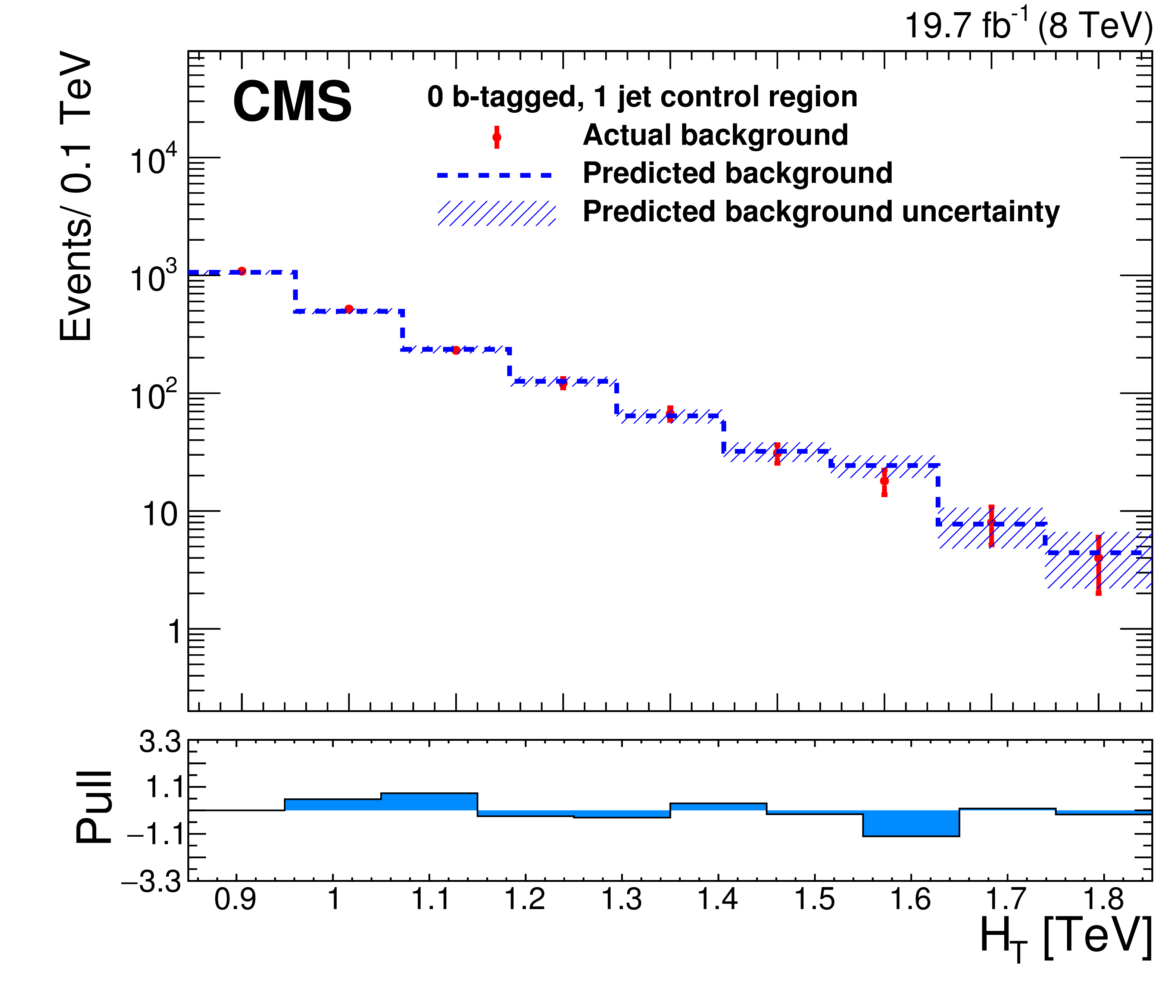
Figure 9-a:
Background closure test in the data control samples of the all-hadronic analysis with no b jets and exactly one AK5 jet with $ {p_{\mathrm {T}}} > $ 80 GeV (a) and with $\ge $2 AK5 jets with $ {p_{\mathrm {T}}} > $ 80 GeV (b). The red data points represent the actual background as derived from data. The blue dashed line represents the predicted background, with the hatched area depicting the corresponding uncertainty. The difference between the observed and predicted background divided by the total uncertainty in the background prediction (pull) is shown for each bin in the lower panels. |
png pdf |
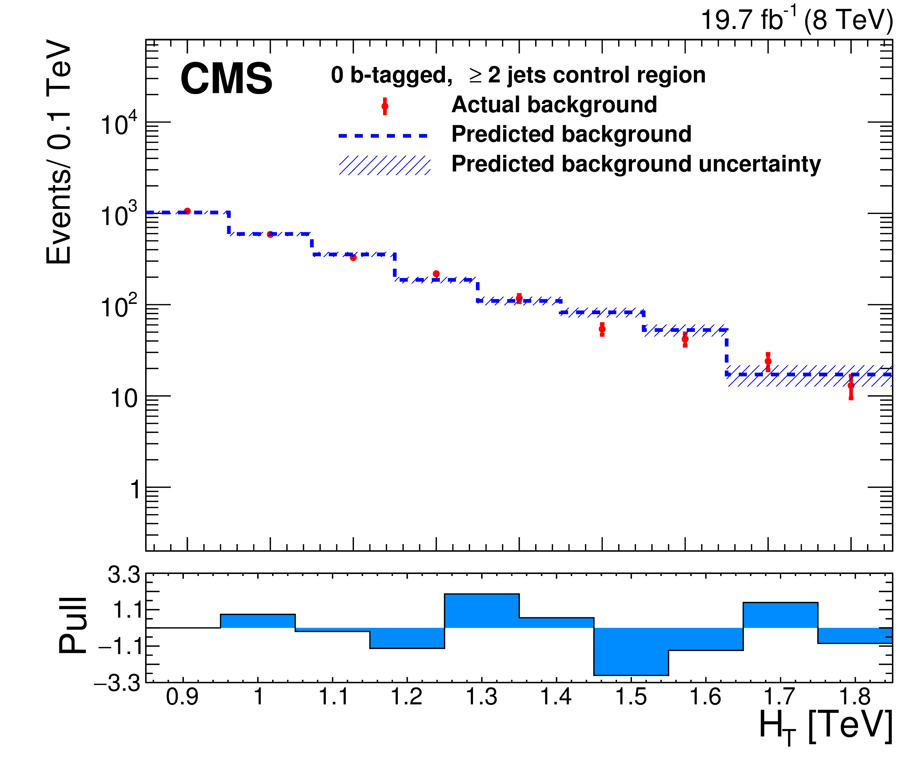
Figure 9-b:
Background closure test in the data control samples of the all-hadronic analysis with no b jets and exactly one AK5 jet with $ {p_{\mathrm {T}}} > $ 80 GeV (a) and with $\ge $2 AK5 jets with $ {p_{\mathrm {T}}} > $ 80 GeV (b). The red data points represent the actual background as derived from data. The blue dashed line represents the predicted background, with the hatched area depicting the corresponding uncertainty. The difference between the observed and predicted background divided by the total uncertainty in the background prediction (pull) is shown for each bin in the lower panels. |
png pdf |
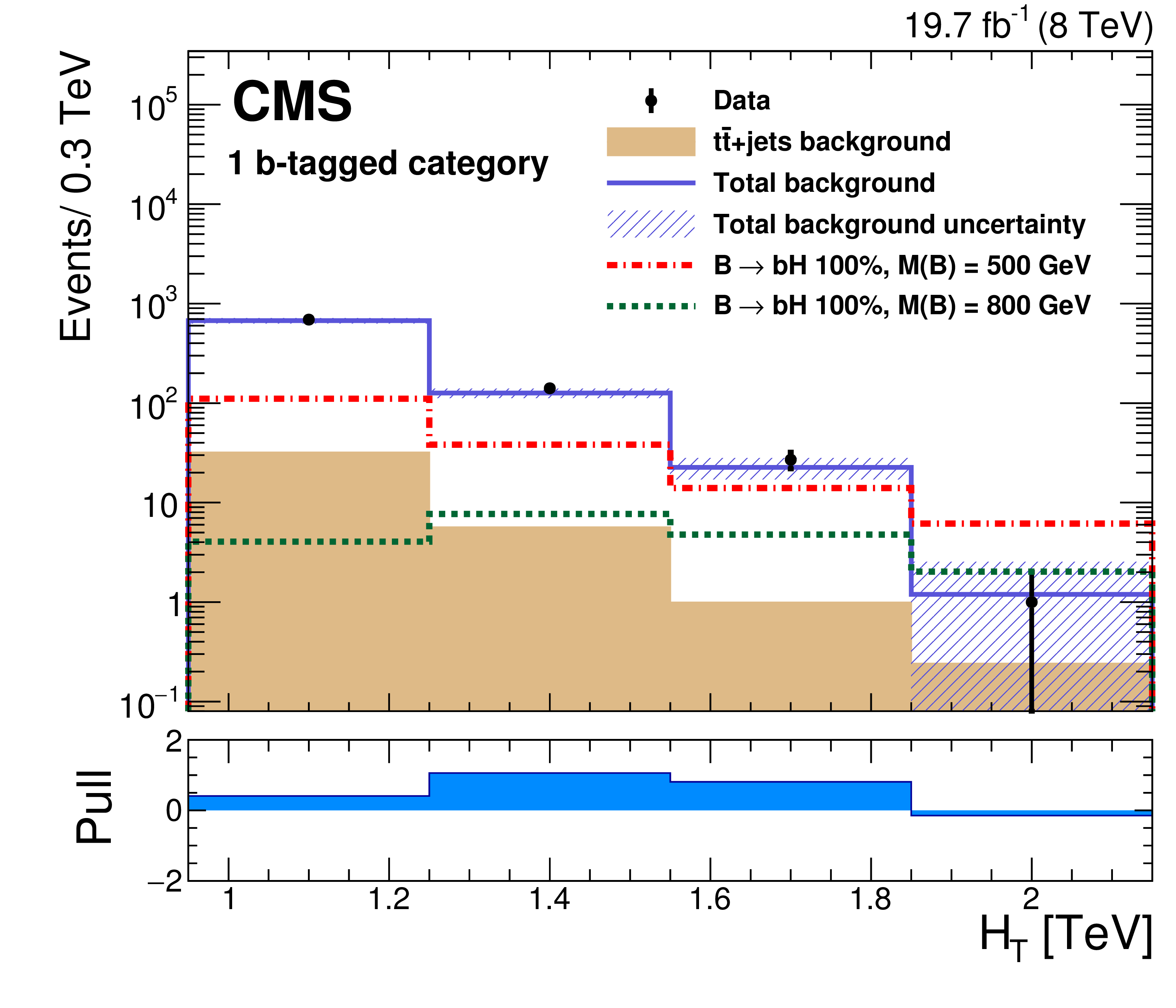
Figure 10-a:
The ${H_{\mathrm {T}}}$ distributions in the 1 b jet (a) and the $\ge $2 b jets event categories (b) for the all-hadronic analysis. The blue solid line depicts the estimated background, with the hatched area showing the measured uncertainty in the background. The signal contributions for two B quark mass points, 500 and 800 GeV , are overlaid. The bin width is chosen to have a statistically significant number of events in every bin. The difference between the data and the estimated background divided by the total uncertainty in the background (pull) is shown for each bin in the lower panels. |
png pdf |
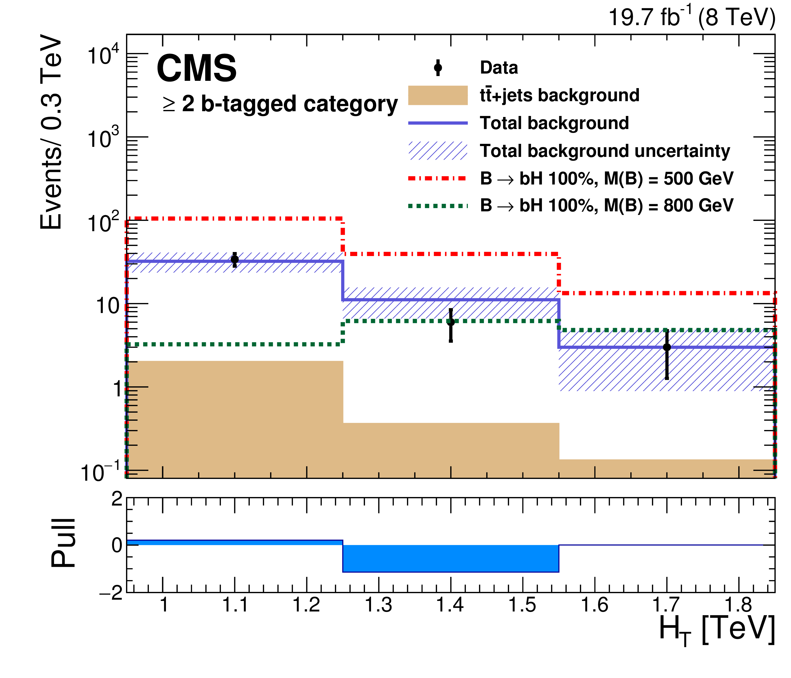
Figure 10-b:
The ${H_{\mathrm {T}}}$ distributions in the 1 b jet (a) and the $\ge $2 b jets event categories (b) for the all-hadronic analysis. The blue solid line depicts the estimated background, with the hatched area showing the measured uncertainty in the background. The signal contributions for two B quark mass points, 500 and 800 GeV , are overlaid. The bin width is chosen to have a statistically significant number of events in every bin. The difference between the data and the estimated background divided by the total uncertainty in the background (pull) is shown for each bin in the lower panels. |
png pdf |
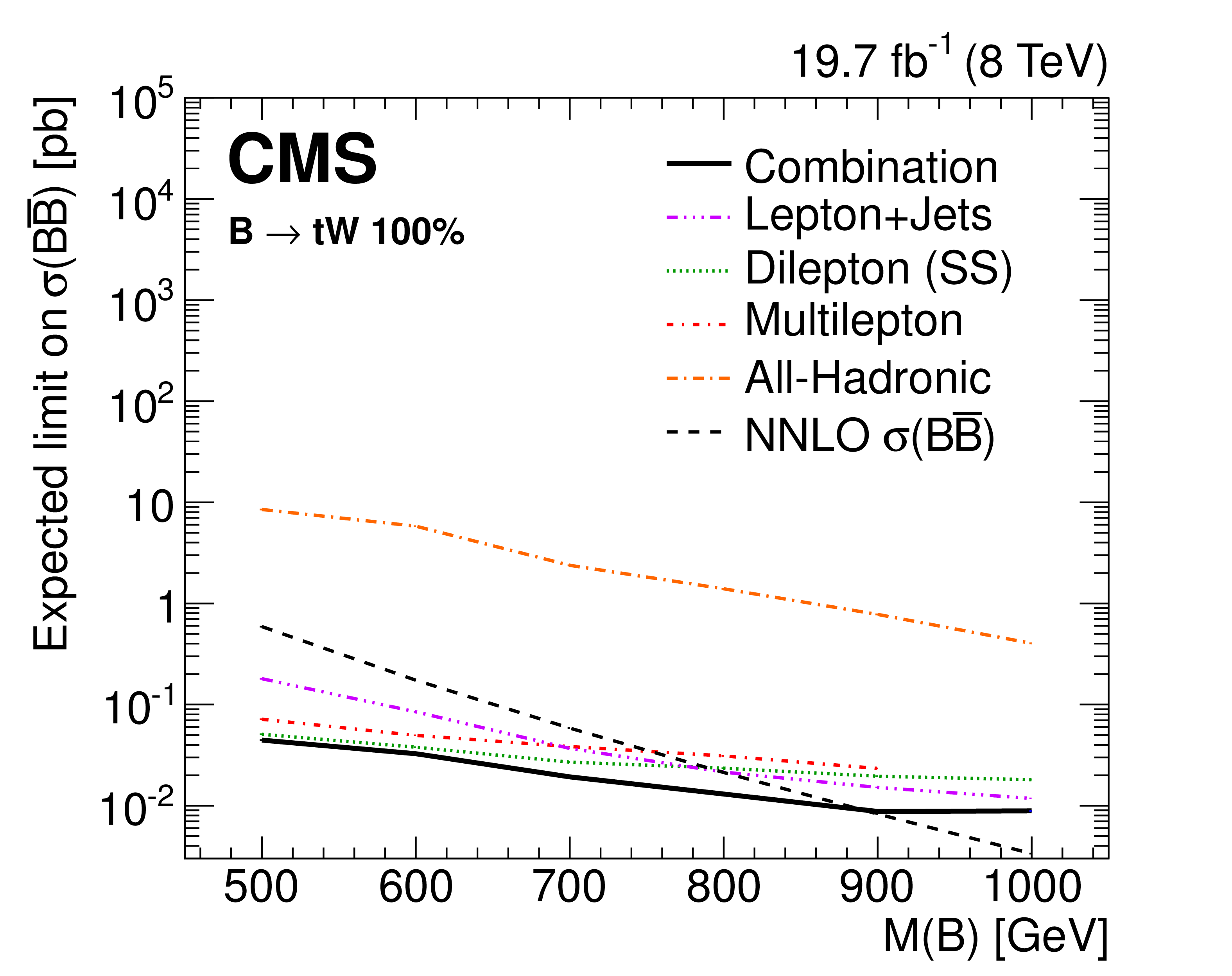
Figure 11-a:
Comparison of individual channel limit results with those of the combination, for the expected limits only. Shown are the limit results, at 95% CL , for the three corners of the triangular parameter space, for 100% branching fractions for B to $\mathrm{ t } \mathrm{ W } $ (a), $\mathrm{ b } {\mathrm{ Z } } $ (b), and $\mathrm{ b } \mathrm{ H } $ (c). The same-sign and opposite-sign channels are denoted by ``SS'' and ``OS'', respectively. The step observed in the $\mathrm{ b } {\mathrm{ Z } } $ limit curve is due to two analysis channels (multilepton and OS dilepton) that do not contribute to the combination for B quark masses above 800 GeV. |
png pdf |
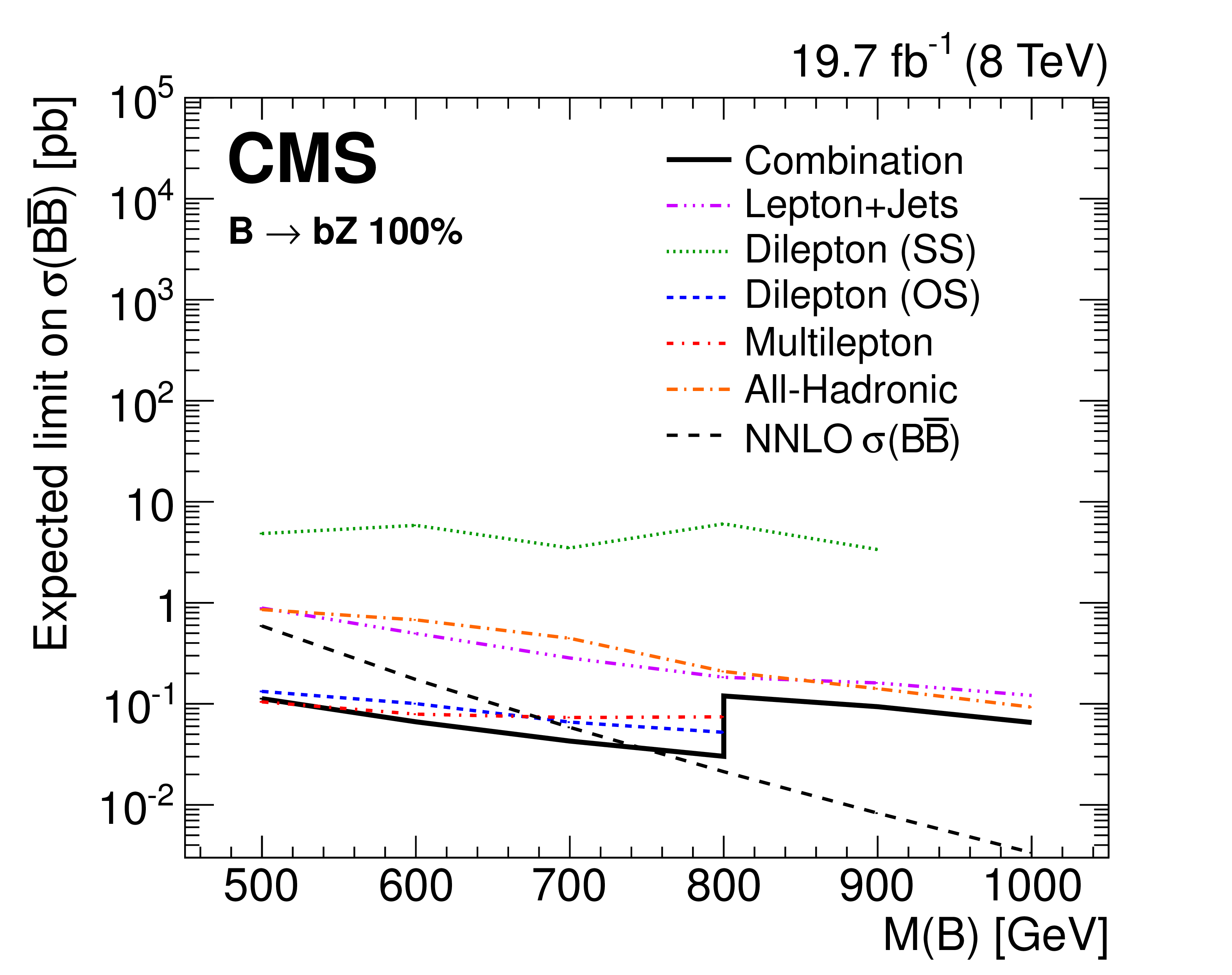
Figure 11-b:
Comparison of individual channel limit results with those of the combination, for the expected limits only. Shown are the limit results, at 95% CL , for the three corners of the triangular parameter space, for 100% branching fractions for B to $\mathrm{ t } \mathrm{ W } $ (a), $\mathrm{ b } {\mathrm{ Z } } $ (b), and $\mathrm{ b } \mathrm{ H } $ (c). The same-sign and opposite-sign channels are denoted by ``SS'' and ``OS'', respectively. The step observed in the $\mathrm{ b } {\mathrm{ Z } } $ limit curve is due to two analysis channels (multilepton and OS dilepton) that do not contribute to the combination for B quark masses above 800 GeV. |
png pdf |
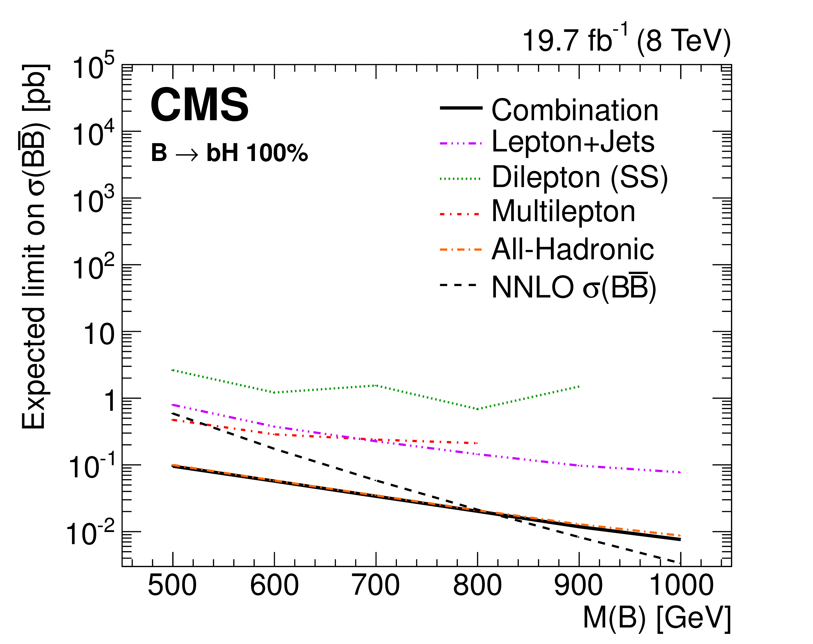
Figure 11-c:
Comparison of individual channel limit results with those of the combination, for the expected limits only. Shown are the limit results, at 95% CL , for the three corners of the triangular parameter space, for 100% branching fractions for B to $\mathrm{ t } \mathrm{ W } $ (a), $\mathrm{ b } {\mathrm{ Z } } $ (b), and $\mathrm{ b } \mathrm{ H } $ (c). The same-sign and opposite-sign channels are denoted by ``SS'' and ``OS'', respectively. The step observed in the $\mathrm{ b } {\mathrm{ Z } } $ limit curve is due to two analysis channels (multilepton and OS dilepton) that do not contribute to the combination for B quark masses above 800 GeV. |
png pdf |
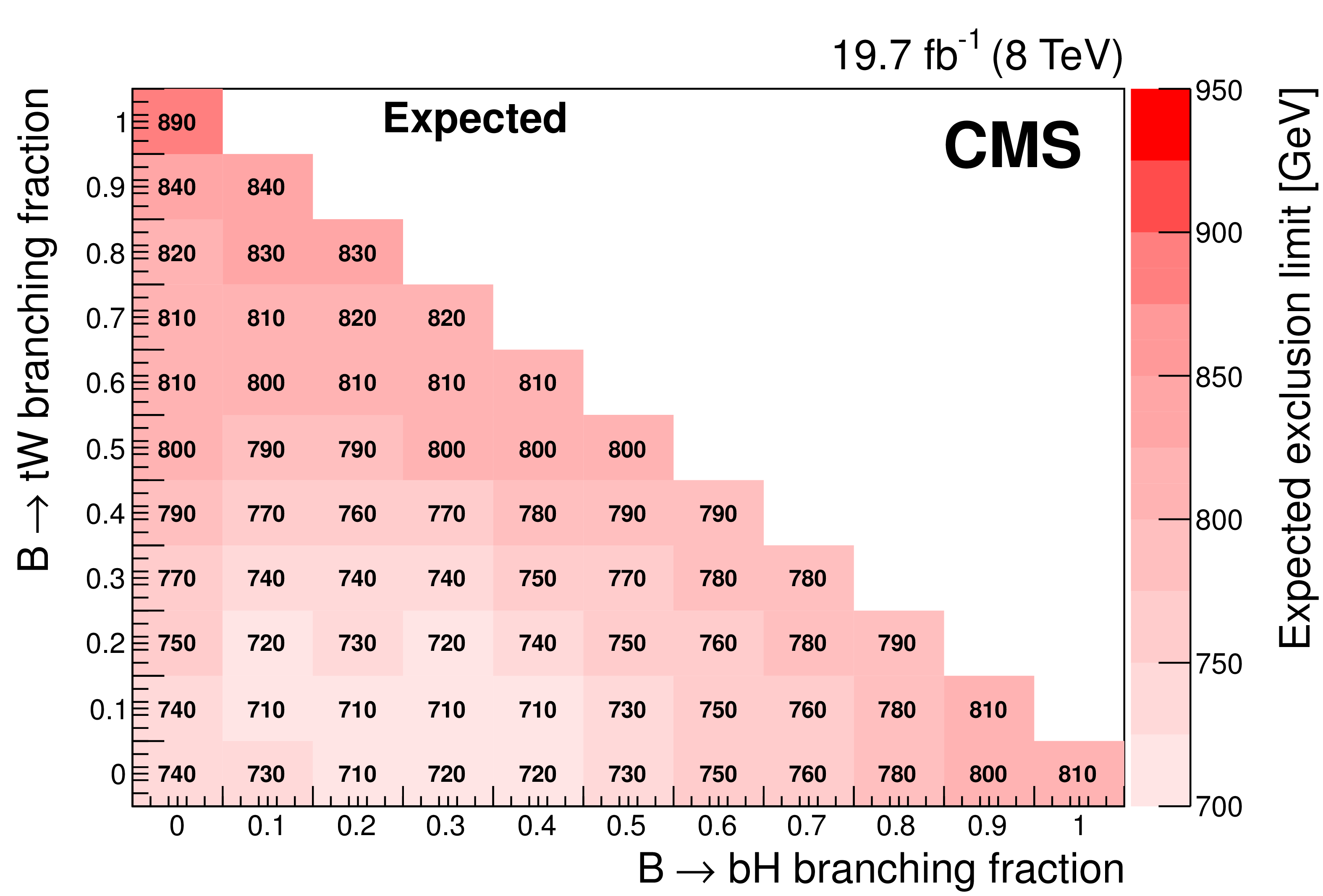
Figure 12-a:
Expected (a) and observed (b) limits for each combination of branching fractions to $\mathrm{ t } \mathrm{ W } $, $\mathrm{ b } {\mathrm{ Z } } $, and $\mathrm{ b } \mathrm{ H } $ obtained by the combination of channels. The color scale represents the mass exclusion limit obtained at each point. The branching fraction for the B quark decay to $\mathrm{ b } {\mathrm{ Z } } $ can be obtained through the relation $\mathcal {B}(\mathrm{ b } {\mathrm{ Z } } ) = 1 - \mathcal {B}(\mathrm{ t } \mathrm{ W } ) - \mathcal {B}(\mathrm{ b } \mathrm{ H } )$. |
png pdf |
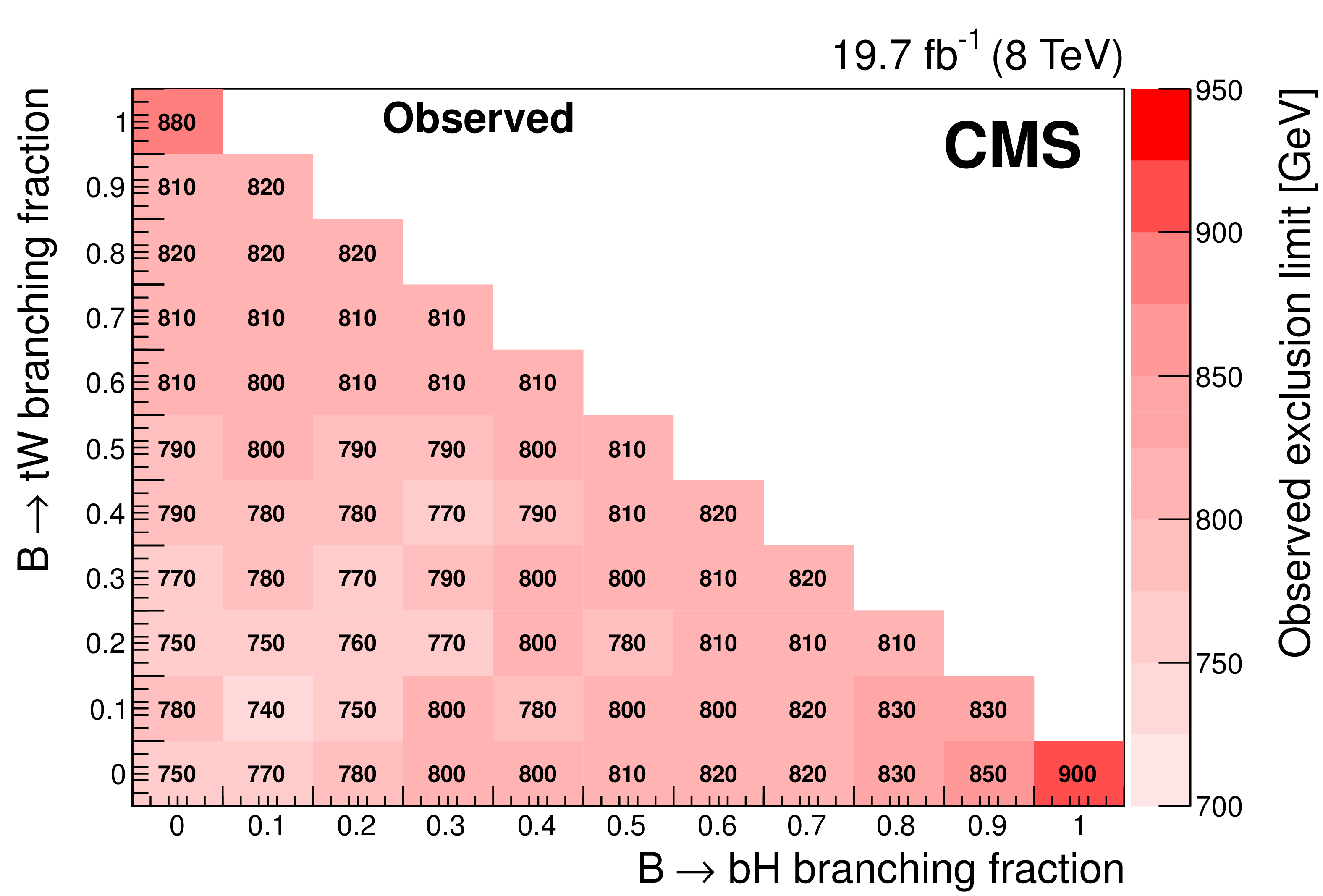
Figure 12-b:
Expected (a) and observed (b) limits for each combination of branching fractions to $\mathrm{ t } \mathrm{ W } $, $\mathrm{ b } {\mathrm{ Z } } $, and $\mathrm{ b } \mathrm{ H } $ obtained by the combination of channels. The color scale represents the mass exclusion limit obtained at each point. The branching fraction for the B quark decay to $\mathrm{ b } {\mathrm{ Z } } $ can be obtained through the relation $\mathcal {B}(\mathrm{ b } {\mathrm{ Z } } ) = 1 - \mathcal {B}(\mathrm{ t } \mathrm{ W } ) - \mathcal {B}(\mathrm{ b } \mathrm{ H } )$. |
png pdf |
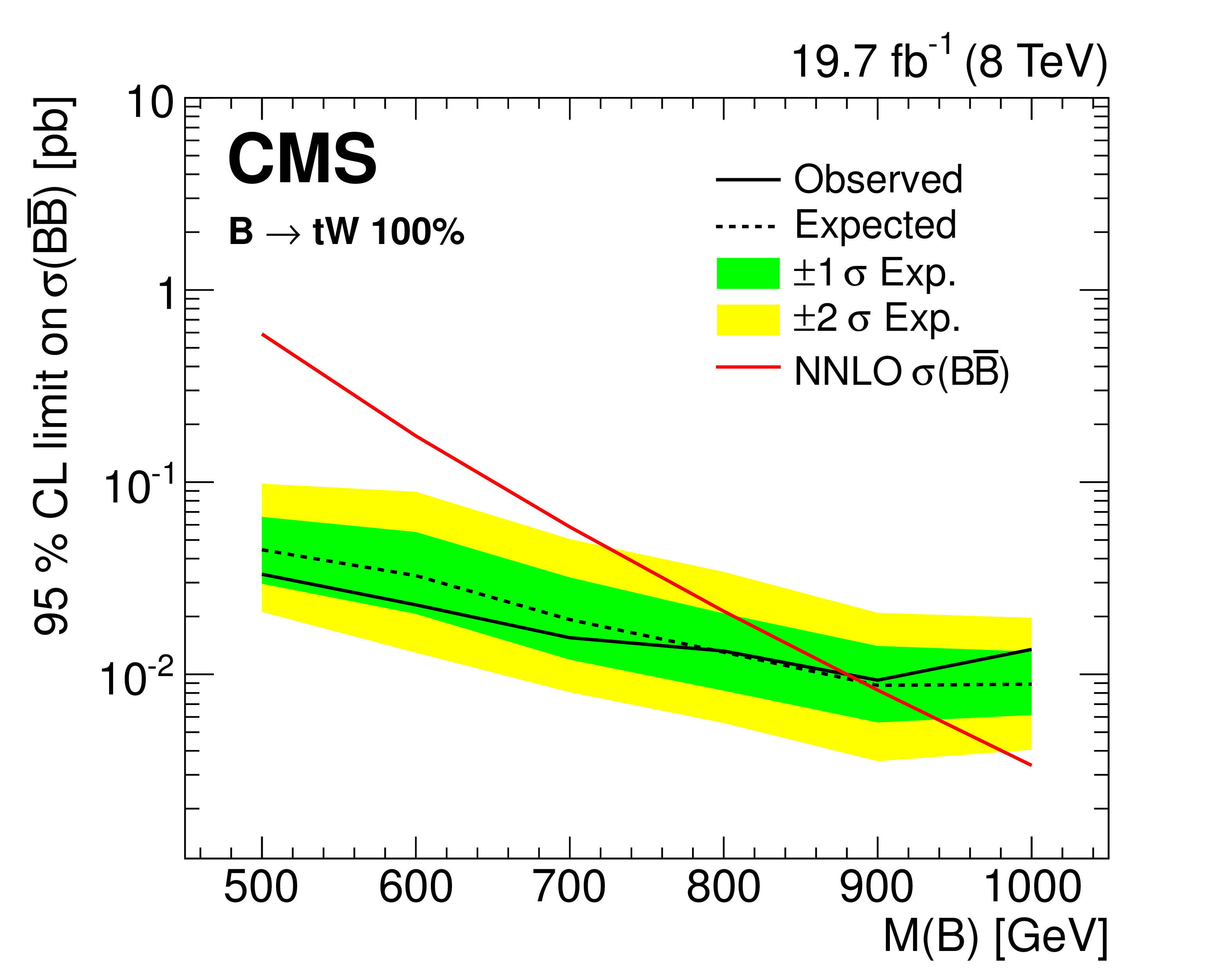
Figure 13-a:
Observed and expected cross section limit results as a function of B mass, for the combination of all channels. The limit results are shown for exclusive branching fractions of B to $\mathrm{ t } \mathrm{ W } $ (a), $\mathrm{ b } {\mathrm{ Z } } $ (b), and $\mathrm{ b } \mathrm{ H } $ (c). The step observed in the $\mathrm{ b } {\mathrm{ Z } } $ limit curve is due to two analysis channels (multilepton and OS dilepton) that do not contribute to the combination for B quark masses above 800 GeV. |
png pdf |
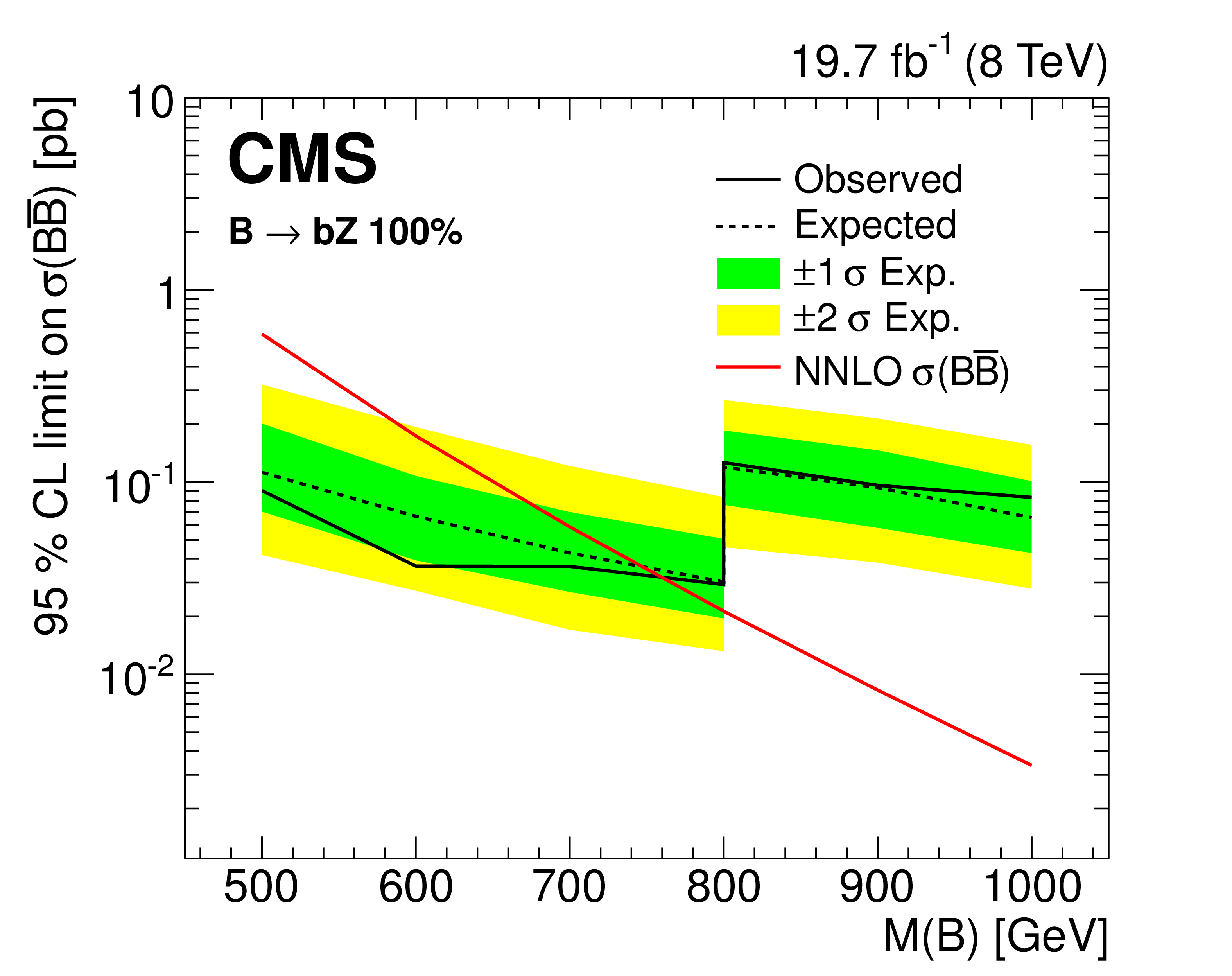
Figure 13-b:
Observed and expected cross section limit results as a function of B mass, for the combination of all channels. The limit results are shown for exclusive branching fractions of B to $\mathrm{ t } \mathrm{ W } $ (a), $\mathrm{ b } {\mathrm{ Z } } $ (b), and $\mathrm{ b } \mathrm{ H } $ (c). The step observed in the $\mathrm{ b } {\mathrm{ Z } } $ limit curve is due to two analysis channels (multilepton and OS dilepton) that do not contribute to the combination for B quark masses above 800 GeV. |
png pdf |
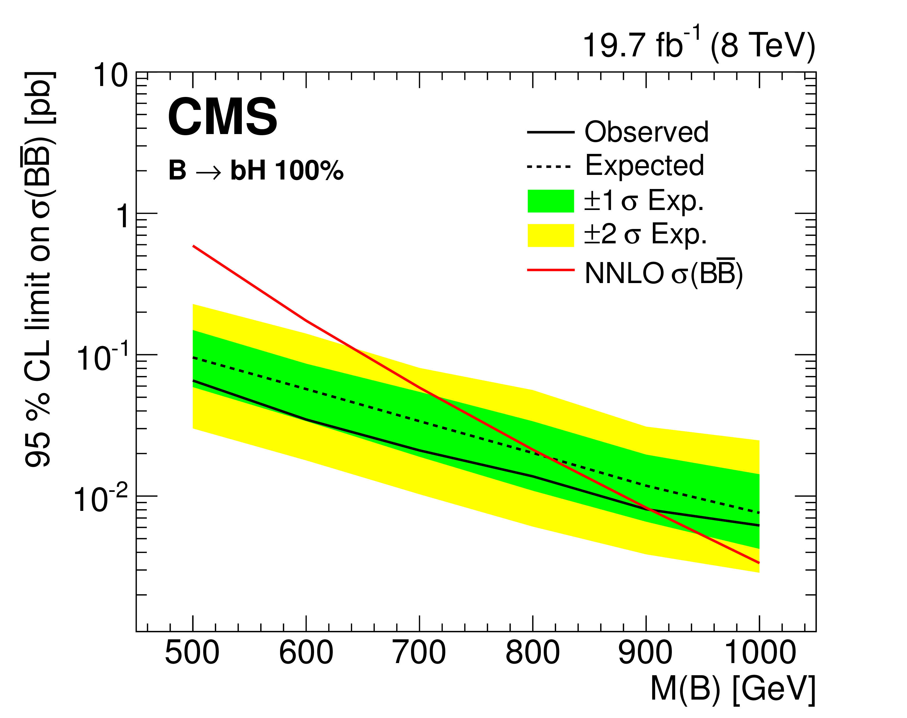
Figure 13-c:
Observed and expected cross section limit results as a function of B mass, for the combination of all channels. The limit results are shown for exclusive branching fractions of B to $\mathrm{ t } \mathrm{ W } $ (a), $\mathrm{ b } {\mathrm{ Z } } $ (b), and $\mathrm{ b } \mathrm{ H } $ (c). The step observed in the $\mathrm{ b } {\mathrm{ Z } } $ limit curve is due to two analysis channels (multilepton and OS dilepton) that do not contribute to the combination for B quark masses above 800 GeV. |
| Tables | |
png pdf |
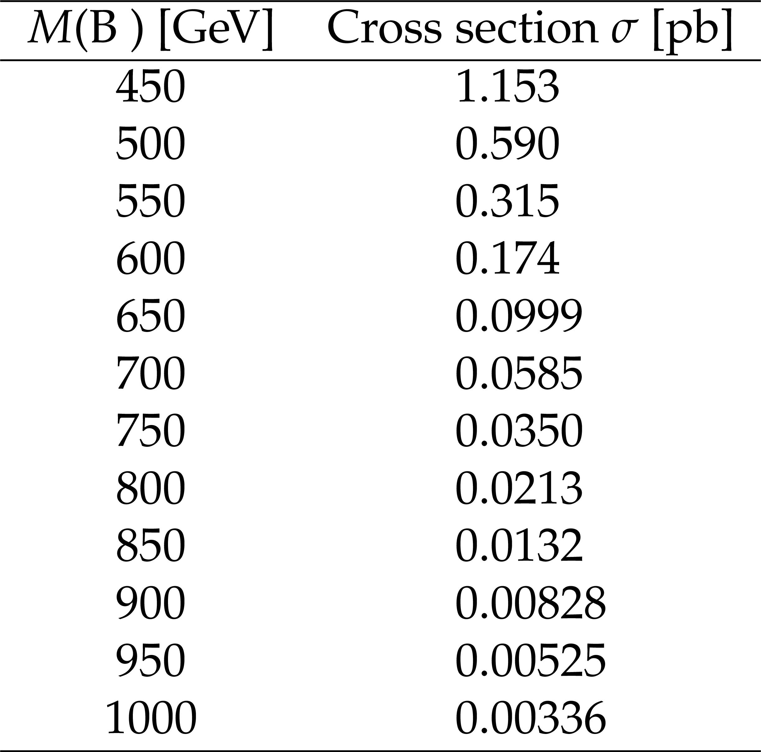
Table 1:
Production cross sections for $\mathrm{ p } \mathrm{ p } \to \mathrm{ B } \mathrm{ \bar{B} } $, used to normalize simulated signal samples to expected event yields. The cross sections are computed to NNLO with Top++2.0 [40]. |
png pdf |
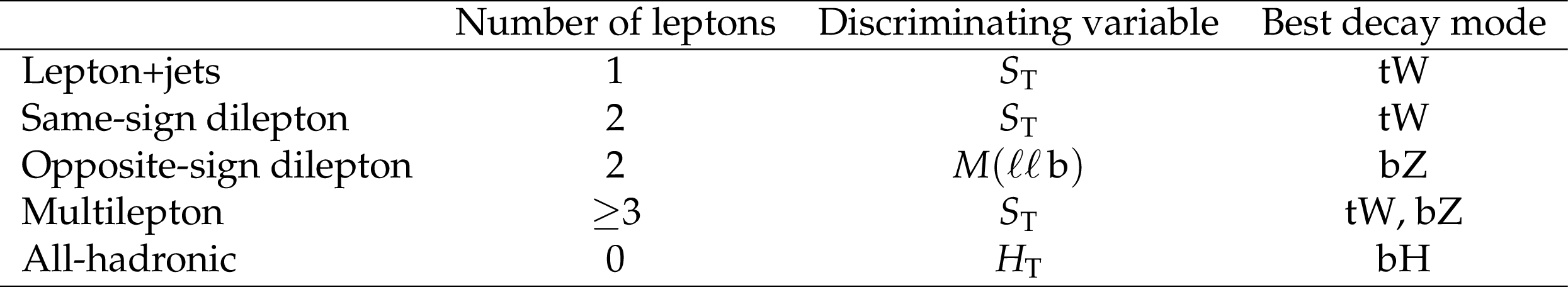
Table 2:
A summary of analysis channels entering the combination, along with the number of selected leptons, the variable used for signal discrimination, and the B quark decay mode providing the best sensitivity for the channel. |
png pdf |
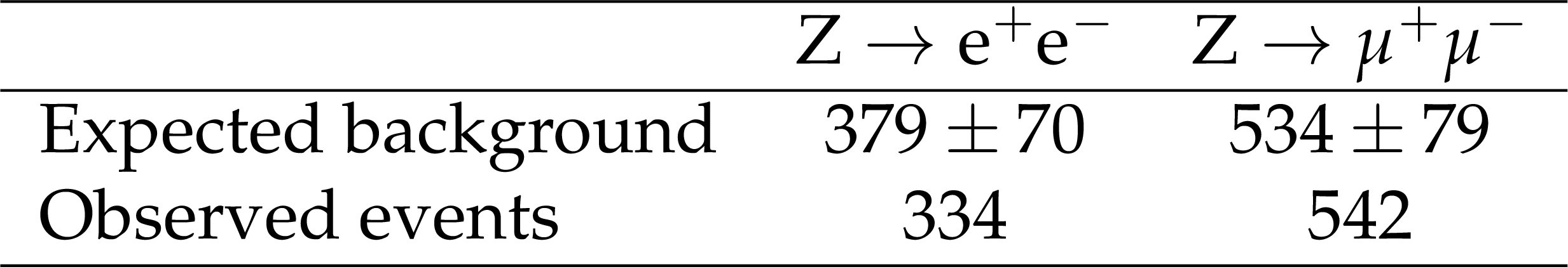
Table 3:
Expected background yields and observed number of events in data in the opposite-sign dilepton channel. The background is obtained from data. The background uncertainties include both statistical and systematic components. |
png pdf |
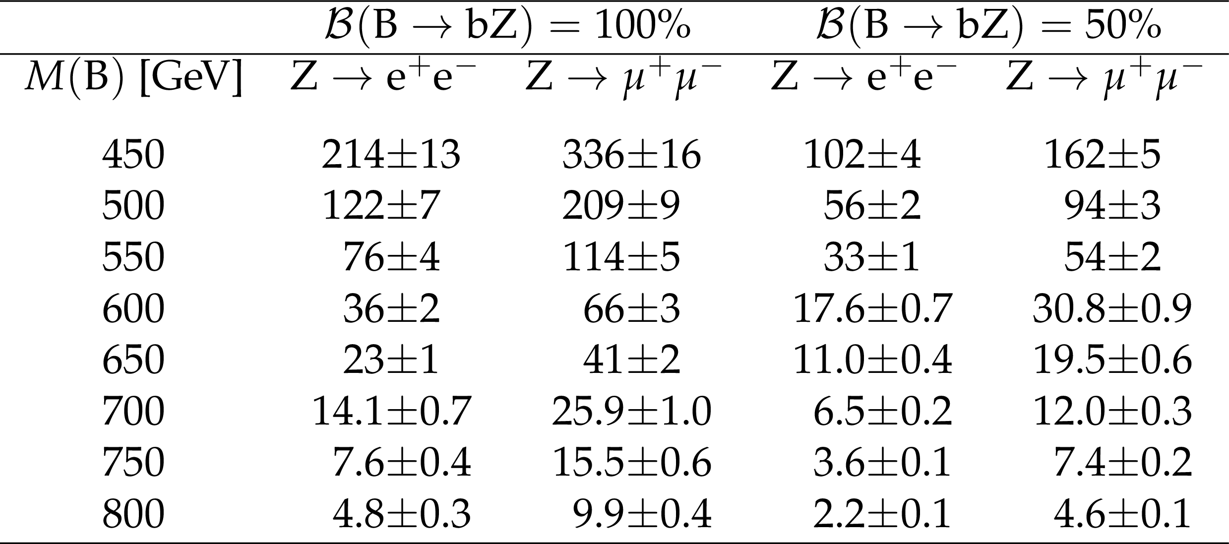
Table 4:
Expected signal event yields in the opposite-sign dilepton channel, shown for B quark masses $M(\mathrm{ B } )$ from 450 to 800 GeV and for two values of the branching fraction. |
png pdf |
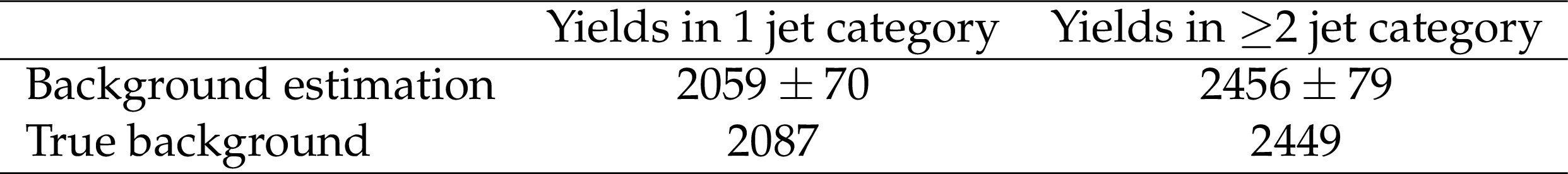
Table 5:
Closure test of the background estimation method for the all-hadronic channel, in the data using a control sample with no b jets. The background is estimated from the sideband regions $A$, $C$, and $D$. The product $N_A (N_C/N_D)$ is compared with the actual background observed in region $B$ in the data. The uncertainties correspond to the statistical uncertainties from limited sample sizes. The agreement obtained is within the uncertainties. |
png pdf |
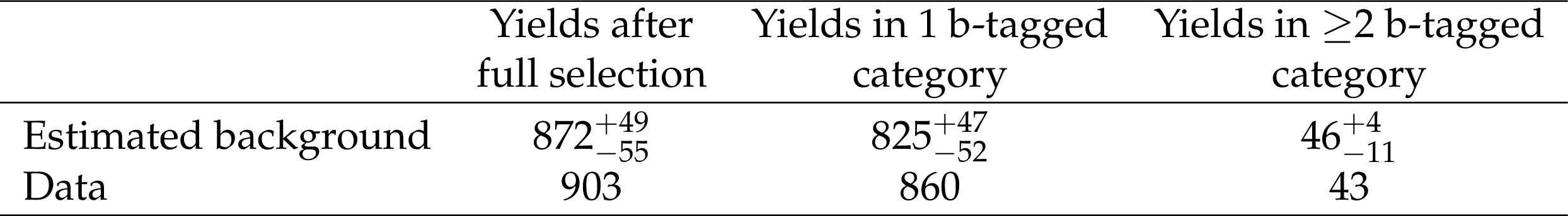
Table 6:
Estimated background and the event yields in the data for the 1 b jet, ${\ge }2$ b jets, and combined event categories in the all-hadronic channel. The uncertainties in the background yields are obtained by propagating the statistical uncertainties from the sideband samples. |
png pdf |
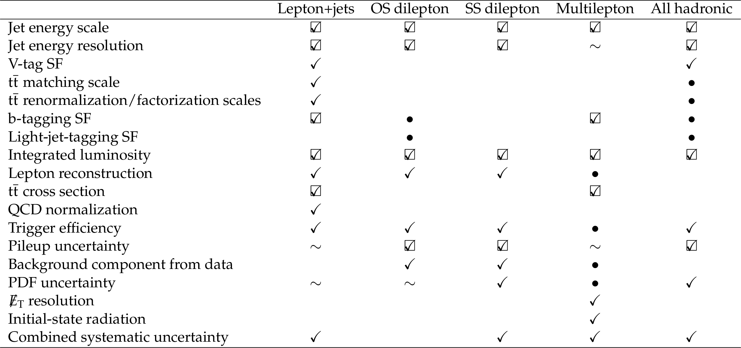
Table 7:
Nuisance parameters applied to the statistical combination. They are listed separately for each individual channel, and the $v$ symbol is used if they are applied to that given channel. If a nuisance parameter is taken as correlated between channels, the $v$ symbol is shown. In some cases, several systematic uncertainties are combined into a single nuisance parameter (for example, in the case of combined lepton categories); in such instances, the $\bullet $ symbol is used to denote the presence of a systematic uncertainty combined with others in a distinct nuisance parameter. The $\sim $ symbol has been used to denote systematic uncertainties that have negligible effects on the analysis results. The ``Combined systematic uncertainty'' entry represents a contribution composed of other sources listed in the table, applied as a single nuisance parameter during limit extraction. |
png pdf |
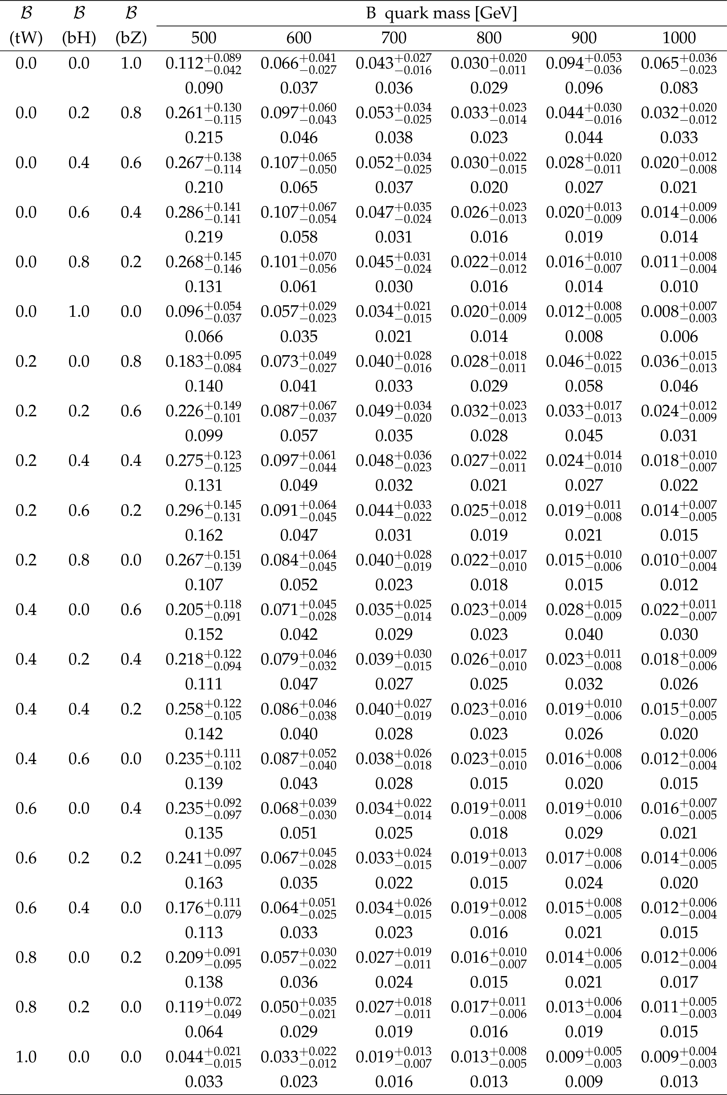
Table 8:
Cross section limits for various combinations of branching fractions and B quark masses. The expected cross section limits are given in the first row for each branching fraction combination, along with their corresponding uncertainties. The observed cross section limits are shown in the second row. All limits are given at 95% CL , and are shown in units of pb. |
png pdf |
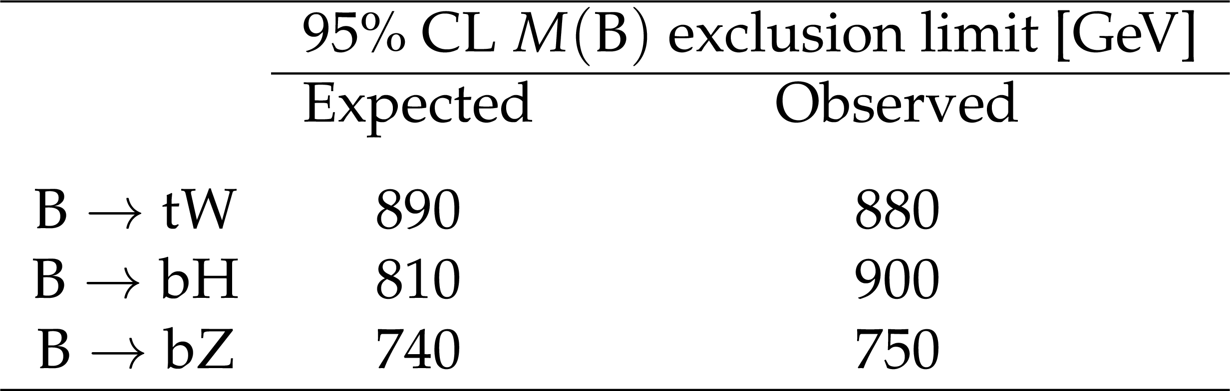
Table 9:
Expected and observed mass exclusion limits for the combined result, quoted at 95% CL , for the topologies where the B quark decays exclusively in one of the possible modes. |
| Summary |
|
A search for pair production of the B quark with vectorlike couplings to W, Z, and Higgs bosons has been performed, using data recorded by the CMS experiment from proton-proton collisions at a center-of-mass energy of 8 TeV at the CERN LHC in 2012. This hypothesized particle could decay in one of three ways: to $\mathrm{ t }\mathrm{ W }$, $\mathrm{ b }\mathrm{ Z }$, or $\mathrm{ b }\mathrm{ H }$. The search is performed using five distinct topologies to maintain sensitivity to each of these decay modes. The topologies included in this search are the lepton+jets final state, both the opposite-sign and same-sign lepton pair final states, the three or more leptons final state, and finally the all-hadronic final state targeting Higgs boson decays to pairs of bottom quarks. No evidence for the production of B quarks in any topology is found, and limits are set on the B quark-antiquark pair-production cross section. A scan over possible combinations of the branching fractions to $\mathrm{ t }\mathrm{ W }$, $\mathrm{ b }\mathrm{ Z }$, and $\mathrm{ b }\mathrm{ H }$ is performed. For a B quark decaying with a branching fraction of 100% to $\mathrm{ b }\mathrm{ H }$, B quarks with masses up to 900 GeV are excluded, at 95% confidence level. This branching fraction corresponds to the highest excluded B quark mass in this scan. Observed exclusion limit results from a scan of all possible branching fractions range from a minimum of 740 GeV to 900 GeV. The combination of these results provides the most stringent exclusion limit to date for the existence of a vectorlike B quark. |
| References | ||||
| 1 | CMS Collaboration | Observation of a new boson with mass near 125 GeV in pp collisions at $ \sqrt{s} $ = 7 and 8 TeV | JHEP 06 (2013) 081 | CMS-HIG-12-036 1303.4571 |
| 2 | ATLAS Collaboration | Observation of a new particle in the search for the Standard Model Higgs boson with the ATLAS detector at the LHC | PLB 716 (2012) 1 | 1207.7214 |
| 3 | CMS Collaboration | Observation of a new boson at a mass of 125 GeV with the CMS experiment at the LHC | PLB 716 (2012) 30 | CMS-HIG-12-028 1207.7235 |
| 4 | J. Bagger, S. Dimopoulos, and E. Masso | Heavy families: Masses and mixings | Nucl. Phys. B 253 (1985) 397 | |
| 5 | K. Agashe, R. Contino, and A. Pomarol | The minimal composite Higgs model | Nucl. Phys. B 719 (2005) 165 | hep-ph/0412089 |
| 6 | R. Contino, Y. Nomura, and A. Pomarol | Higgs as a holographic pseudo-Goldstone boson | Nucl. Phys. B 671 (2003) 148 | hep-ph/0306259 |
| 7 | J. Berger, J. Hubisz, and M. Perelstein | A fermionic top partner: naturalness and the LHC | JHEP 07 (2012) 016 | 1205.0013 |
| 8 | T. Han, H. E. Logan, and L.-T. Wang | Smoking-gun signatures of little Higgs models | JHEP 01 (2006) 099 | hep-ph/0506313 |
| 9 | M. Perelstein, M. E. Peskin, and A. Pierce | Top quarks and electroweak symmetry breaking in little Higgs models | PRD 69 (2004) 075002 | hep-ph/0310039 |
| 10 | N. Arkani-Hamed et al. | The Minimal Moose for a Little Higgs | JHEP 08 (2002) 021 | hep-ph/0206020 |
| 11 | B. A. Dobrescu and C. T. Hill | Electroweak symmetry breaking via top condensation seesaw | PRL 81 (1998) 2634 | hep-ph/9712319 |
| 12 | J. A. Aguilar-Saavedra, R. Benbrik, S. Heinemeyer, and M. P\'erez-Victoria | Handbook of vectorlike quarks: Mixing and single production | PRD 88 (2013) 094010 | |
| 13 | S. Fajfer, A. Greljo, J. F. Kamenik, and I. Mustac | Light Higgs and Vector-like Quarks without Prejudice | JHEP 07 (2013) 155 | 1304.4219 |
| 14 | P. H. Frampton, P. Q. Hung, and M. Sher | Quarks and leptons beyond the third generation | PR 330 (2000) 263 | hep-ph/9903387 |
| 15 | A. Djouadi and A. Lenz | Sealing the fate of a fourth generation of fermions | PLB 715 (2012) 310 | |
| 16 | S. Gopalakrishna, T. Mandal, S. Mitra, and R. Tibrewala | LHC signatures of a vector-like $ b' $ | PRD 84 (2011) 055001 | 1107.4306 |
| 17 | J. A. Aguilar-Saavedra | Identifying top partners at LHC | JHEP 11 (2009) 030 | 0907.3155 |
| 18 | Y. Okada and L. Panizzi | LHC signatures of vector-like quarks | Adv. High Energy Phys. 2013 (2013) 364936 | 1207.5607 |
| 19 | P. Agrawal, S. D. Ellis, and W.-S. Hou | Q$ \to $qZ decays at Tevatron and SSC energies | PLB 256 (1991) 289 | |
| 20 | S. P. Martin | Extra vector-like matter and the lightest Higgs scalar boson mass in low-energy supersymmetry | PRD 81 (2010) 035004 | 0910.2732 |
| 21 | CDF Collaboration | Search for new particles leading to $ Z+ $jets final states in $ p\bar{p} $ collisions at $ \sqrt{s} = 1.96 $ TeV | PRD 76 (2007) 072006 | 0706.3264 |
| 22 | ATLAS Collaboration | Search for production of vector-like quark pairs and of four top quarks in the lepton-plus-jets final state in pp collisions at $ \sqrt{s}=8 $ TeV with the ATLAS detector | JHEP 08 (2015) 105 | 1505.04306v2 |
| 23 | CMS Collaboration | The CMS experiment at the CERN LHC | JINST 3 (2008) S08004 | CMS-00-001 |
| 24 | F. Maltoni and T. Stelzer | MadEvent: automatic event generation with MadGraph | JHEP 02 (2003) 027 | hep-ph/0208156 |
| 25 | J. Pumplin et al. | New generation of parton distributions with uncertainties from global QCD analysis | JHEP 07 (2002) 012 | hep-ph/0201195 |
| 26 | T. Sj\"ostrand, S. Mrenna, and P. Skands | PYTHIA 6.4 physics and manual | JHEP 05 (2006) 026 | hep-ph/0603175 |
| 27 | P. Nason | A new method for combining NLO QCD with shower Monte Carlo algorithms | JHEP 11 (2004) 040 | hep-ph/0409146 |
| 28 | S. Frixione, P. Nason, and C. Oleari | Matching NLO QCD computations with Parton Shower simulations: the POWHEG method | JHEP 11 (2007) 070 | 0709.2092 |
| 29 | S. Alioli, P. Nason, C. Oleari, and E. Re | A general framework for implementing NLO calculations in shower Monte Carlo programs: the POWHEG BOX | JHEP 06 (2010) 043 | 1002.2581 |
| 30 | S. Alioli, P. Nason, C. Oleari, and E. Re | NLO single-top production matched with shower in POWHEG: $ s $- and $ t $-channel contributions | JHEP 09 (2009) 111, , [Erratum: \DOI10.1007/JHEP02(2010)011] | 0907.4076 |
| 31 | R. Gavin, Y. Li, F. Petriello, and S. Quackenbush | FEWZ 2.0: A code for hadronic Z production at next-to-next-to-leading order | CPC 182 (2011) 2388 | 1011.3540 |
| 32 | R. Gavin, Y. Li, F. Petriello, and S. Quackenbush | W Physics at the LHC with FEWZ 2.1 | CPC 184 (2013) 208 | 1201.5896 |
| 33 | Y. Li and F. Petriello | Combining QCD and electroweak corrections to dilepton production in FEWZ | PRD 86 (2012) 094034 | 1208.5967 |
| 34 | M. Czakon, P. Fiedler, and A. Mitov | Total Top-Quark Pair-Production Cross Section at Hadron Colliders Through $ O(\alpha_s^4) $ | PRL 110 (2013) 252004 | 1303.6254 |
| 35 | N. Kidonakis | NNLL threshold resummation for top-pair and single-top production | Phys. Part. Nucl. 45 (2014) 714 | 1210.7813 |
| 36 | J. M. Campbell, R. K. Ellis, and K. Williams | Vector boson pair production at the LHC | JHEP 07 (2011) 018 | 1105.0020 |
| 37 | J. M. Campbell and R. K. Ellis | t$ \overline {\rm t} $ W$ ^{\pm } $ production and decay at NLO | JHEP 07 (2012), no. 052 | |
| 38 | M. V. Garzelli, A. Kardos, C. G. Papadopoulos, and Z. Tr\'ocs\'anyi | $ \mathrm{t} \bar{\mathrm{t}} \mathrm{W}^\pm + \mathrm{t} \bar{\mathrm{t}}\mathrm{Z} $ hadroproduction at NLO accuracy in QCD with Parton Shower and Hadronization effects | JHEP 11 (2012), no. 056 | |
| 39 | M. Aliev et al. | HATHOR: HAdronic Top and Heavy quarks crOss section calculatoR | CPC 182 (2011) 1034 | 1007.1327 |
| 40 | M. Cacciari et al. | Top-pair production at hadron colliders with next-to-next-to-leading logarithmic soft-gluon resummation | PLB 710 (2012) 612 | 1111.5869 |
| 41 | CMS Collaboration | Particle--Flow Event Reconstruction in CMS and Performance for Jets, Taus, and $ E_{\mathrm{T}}^{\text{miss}} $ | CDS | |
| 42 | CMS Collaboration | Commissioning of the Particle-flow Event Reconstruction with the first LHC collisions recorded in the CMS detector | CDS | |
| 43 | CMS Collaboration | Performance of electron reconstruction and selection with the CMS detector in proton-proton collisions at $ \sqrt{s} = 8 $$ TeV $ | JINST 10 (2015) P06005 | CMS-EGM-13-001 1502.02701 |
| 44 | CMS Collaboration | Performance of CMS muon reconstruction in pp collision events at $ \sqrt{s}=7 $ TeV | JINST 7 (2012) P10002 | CMS-MUO-10-004 1206.4071 |
| 45 | CMS Collaboration | Performance of $ \tau $-lepton reconstruction and identification in CMS | JINST 7 (2012) P01001 | |
| 46 | M. Cacciari and G. P. Salam | Pileup subtraction using jet areas | PLB 659 (2008) 119 | 0707.1378 |
| 47 | CMS Collaboration | Commissioning of the Particle-Flow Reconstruction in Minimum-Bias and Jet Events from $ \mathrm{ p }\mathrm{ p } $ Collisions at 7 TeV | CDS | |
| 48 | M. Cacciari, G. P. Salam, and G. Soyez | The anti-$ k_t $ jet clustering algorithm | JHEP 04 (2008) 063 | 0802.1189 |
| 49 | CMS Collaboration | Determination of Jet Energy Calibration and Transverse Momentum Resolution in CMS | JINST 6 (2011) P11002 | CMS-JME-10-011 1107.4277 |
| 50 | CMS Collaboration | Identification of b-quark jets with the CMS experiment | JINST 8 (2013) 04013 | CMS-BTV-12-001 1211.4462 |
| 51 | CMS Collaboration | Performance of b tagging at $ \sqrt{s}=8 $ TeV in multijet, $ \rm{t}\bar{\rm t} $ and boosted topology events | CMS-PAS-BTV-13-001 | CMS-PAS-BTV-13-001 |
| 52 | Y. L. Dokshitzer, G. D. Leder, S. Moretti, and B. R. Webber | Better jet clustering algorithms | JHEP 08 (1997) 001 | hep-ph/9707323 |
| 53 | M. Wobisch and T. Wengler | Hadronization corrections to jet cross sections in deep-inelastic scattering | DESY-PROC 1999-02 | hep-ph/9907280 |
| 54 | J. M. Butterworth, A. R. Davison, M. Rubin, and G. P. Salam | Jet Substructure as a New Higgs-Search Channel at the Large Hadron Collider | PRL 100 (2008) 242001 | 0802.2470 |
| 55 | S. D. Ellis, C. K. Vermilion, and J. R. Walsh | Recombination algorithms and jet substructure: Pruning as a tool for heavy particle searches | PRD 81 (2010) 094023 | 0912.0033 |
| 56 | J. Thaler and K. Van Tilburg | Identifying boosted objects with N-subjettiness | JHEP 03 (2011) 015 | 1011.2268 |
| 57 | CMS Collaboration | Identification techniques for highly boosted W bosons that decay into hadrons | JHEP 12 (2014) 017 | |
| 58 | CMS Collaboration | CMS Luminosity Based on Pixel Cluster Counting -- Summer 2013 Update | CMS-PAS-LUM-13-001 | CMS-PAS-LUM-13-001 |
| 59 | CMS Collaboration | Measurement of the differential cross section for top quark pair production in pp collisions at $ \sqrt{s} = 8\,\text{TeV} $ | EPJC 75 (2015), no. 11, 542 | CMS-TOP-12-028 1505.04480 |
|
|
Compact Muon Solenoid LHC, CERN |
|

|

|

|

|

|