

Compact Muon Solenoid
LHC, CERN
| CMS-HIG-12-036 ; CERN-PH-EP-2013-035 | ||
| Observation of a new boson with mass near 125 GeV in pp collisions at $\sqrt{s}$ = 7 and 8 TeV | ||
| CMS Collaboration | ||
| 19 March 2013 | ||
| J. High Energy Phys. 06 (2013) 081 | ||
| Abstract: A detailed description is reported of the analysis used by the CMS Collaboration in the search for the standard model Higgs boson in pp collisions at the LHC, which led to the observation of a new boson. The data sample corresponds to integrated luminosities up to 5.1 inverse femtobarns at $\sqrt{s}$ = 7 TeV, and up to 5.3 inverse femtobarns at $\sqrt{s}$ = 8 TeV. The results for five Higgs boson decay modes $\gamma\gamma, ZZ, WW, \tau \tau$, and bb, which show a combined local significance of 5 standard deviations near 125 GeV, are reviewed. A fit to the invariant mass of the two high resolution channels, gamma gamma and ZZ to 4 ell, gives a mass estimate of 125.3 +/- 0.4 (stat) +/- 0.5 (syst) GeV. The measurements are interpreted in the context of the standard model Lagrangian for the scalar Higgs field interacting with fermions and vector bosons. The measured values of the corresponding couplings are compared to the standard model predictions. The hypothesis of custodial symmetry is tested through the measurement of the ratio of the couplings to the W and Z bosons. All the results are consistent, within their uncertainties, with the expectations for a standard model Higgs boson. | ||
| Links: e-print arXiv:1303.4571 [hep-ex] (PDF) ; CDS record ; inSPIRE record ; Public twiki page ; CADI line (restricted) ; | ||
| Figures | |
png pdf |
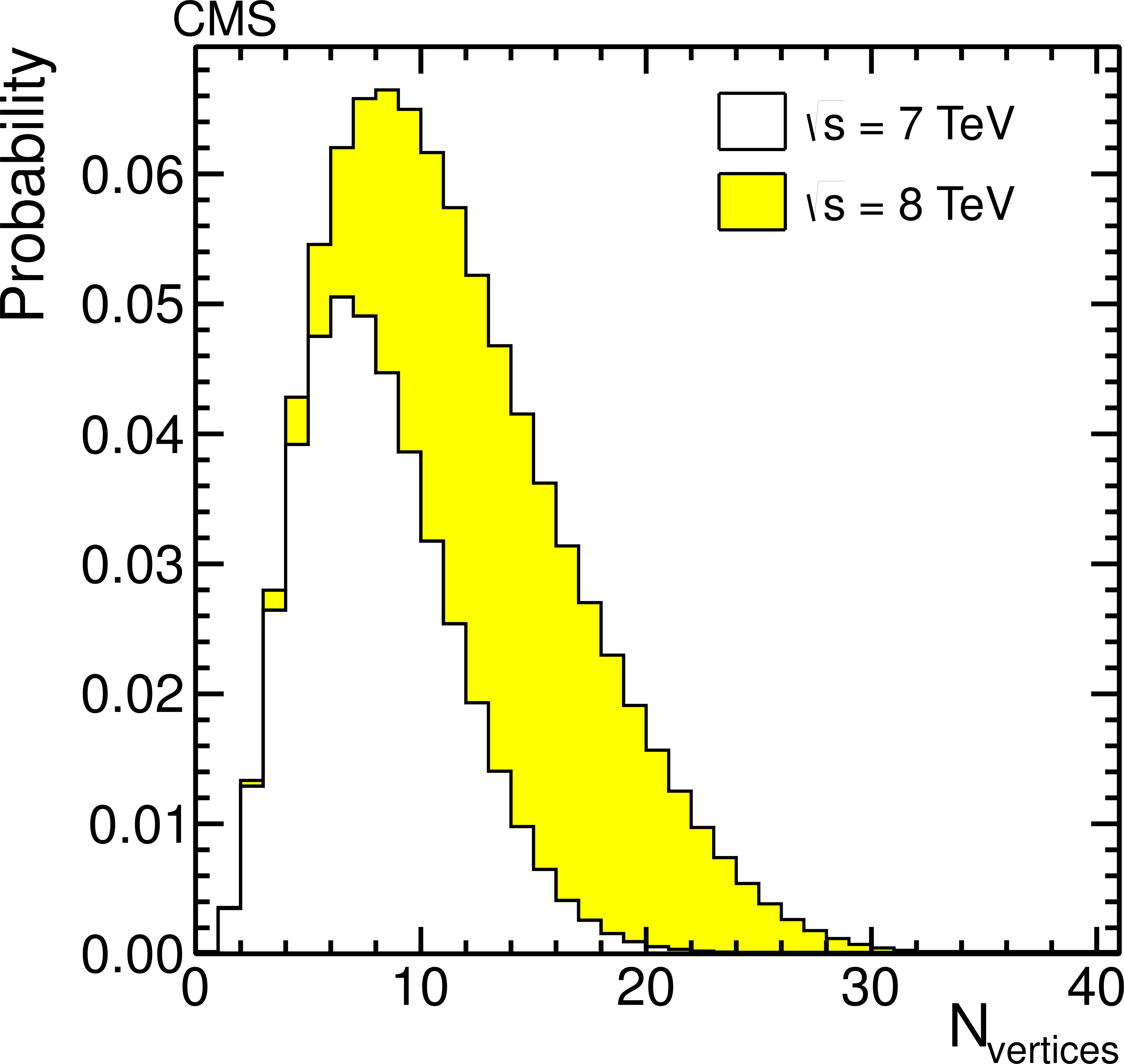
Figure 1-a:
Left: probability distribution for the number of vertices $N_\text {vertices}$ reconstructed per event in the 2011 and 2012 data. The $\sqrt {s}=7$ and $8 TeV $ probability distributions are weighted by their equivalent integrated luminosity, and by the corresponding total cross section $\sigma ( {\mathrm {p}} {\mathrm {p}}\to {\mathrm {H}} +X)$ for a SM Higgs boson of mass 125 GeV . Right: display of a four-lepton event recorded in 2012, with 24 reconstructed vertices. The four leptons are shown as thick lines and originate from the vertex chosen for the hard-scattering process. |
png |
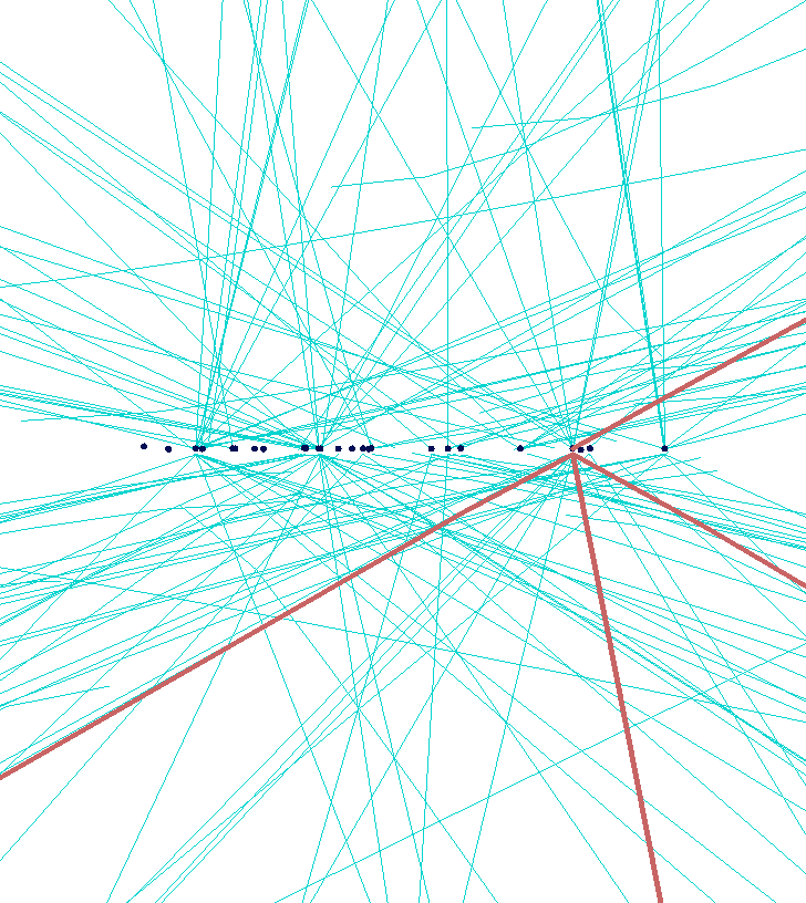
Figure 1-b:
Left: probability distribution for the number of vertices $N_\text {vertices}$ reconstructed per event in the 2011 and 2012 data. The $\sqrt {s}=7$ and $8 TeV $ probability distributions are weighted by their equivalent integrated luminosity, and by the corresponding total cross section $\sigma ( {\mathrm {p}} {\mathrm {p}}\to {\mathrm {H}} +X)$ for a SM Higgs boson of mass 125 GeV . Right: display of a four-lepton event recorded in 2012, with 24 reconstructed vertices. The four leptons are shown as thick lines and originate from the vertex chosen for the hard-scattering process. |

png pdf |
Figure 2-a:
Higgs boson production cross sections at $\sqrt {s}$ = 8 TeV (left) and branching fractions (right) as a function of the Higgs boson mass from Refs.\cite {LHCHiggsCrossSectionWorkingGroup:2011ti,Dittmaier:2012vm}. The width of the lines represents the total theoretical uncertainty in the cross section and in the branching fractions. |

png pdf |
Figure 2-b:
Higgs boson production cross sections at $\sqrt {s}$ = 8 TeV (left) and branching fractions (right) as a function of the Higgs boson mass from Refs.\cite {LHCHiggsCrossSectionWorkingGroup:2011ti,Dittmaier:2012vm}. The width of the lines represents the total theoretical uncertainty in the cross section and in the branching fractions. |

png pdf |
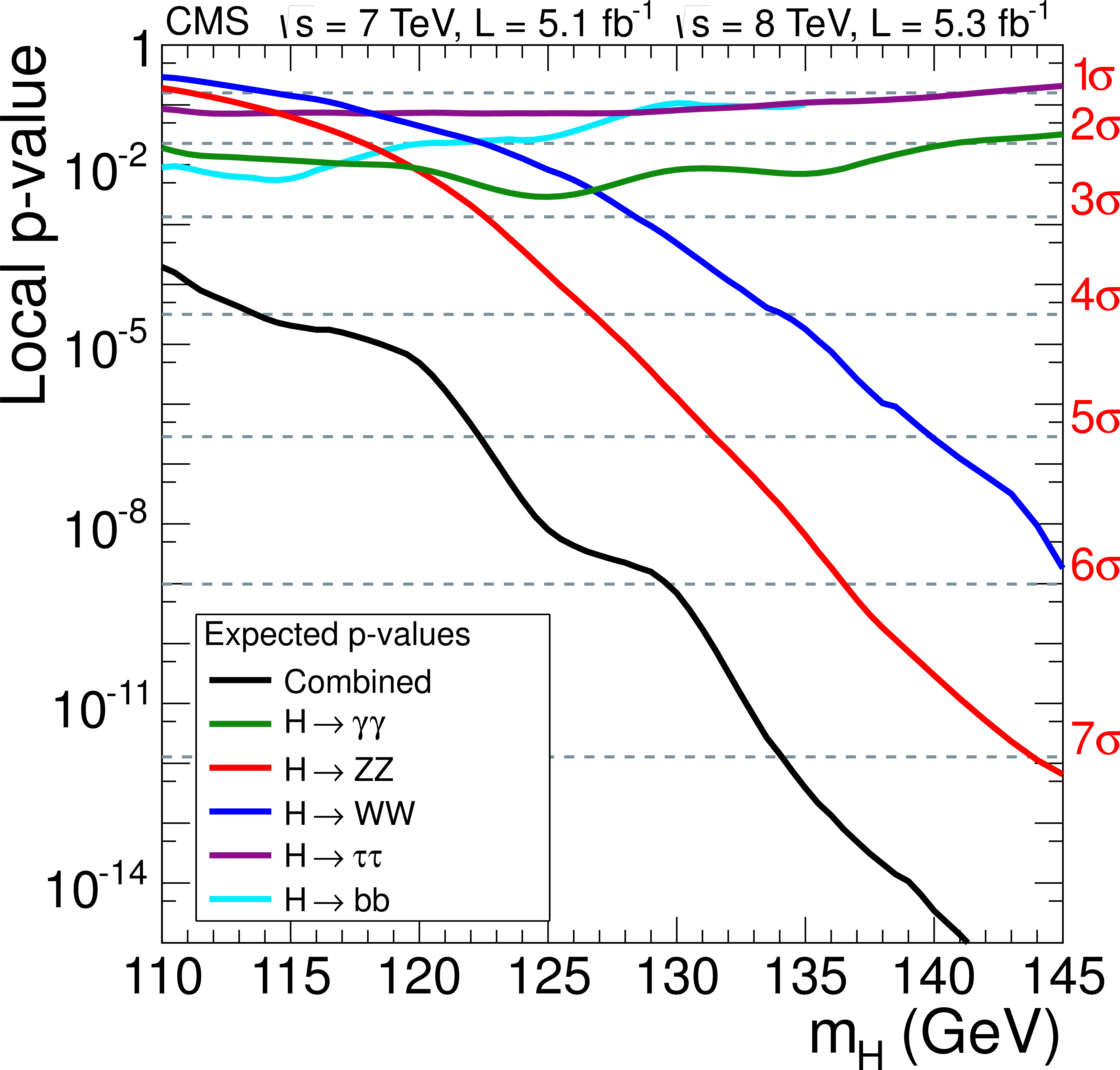
Figure 3-a:
The median expected 95% CL upper limits on the cross section ratio $ \sigma / \sigma _{\mathrm {SM}}$ in the absence of a Higgs boson (left) and the median expected local $p$-value for observing an excess, assuming that a Higgs boson with that mass exists (right), as a function of the Higgs boson mass for the five Higgs boson decay channels and their combination. |
png pdf |
Figure 3-b:
The median expected 95% CL upper limits on the cross section ratio $ \sigma / \sigma _{\mathrm {SM}}$ in the absence of a Higgs boson (left) and the median expected local $p$-value for observing an excess, assuming that a Higgs boson with that mass exists (right), as a function of the Higgs boson mass for the five Higgs boson decay channels and their combination. |
png pdf |
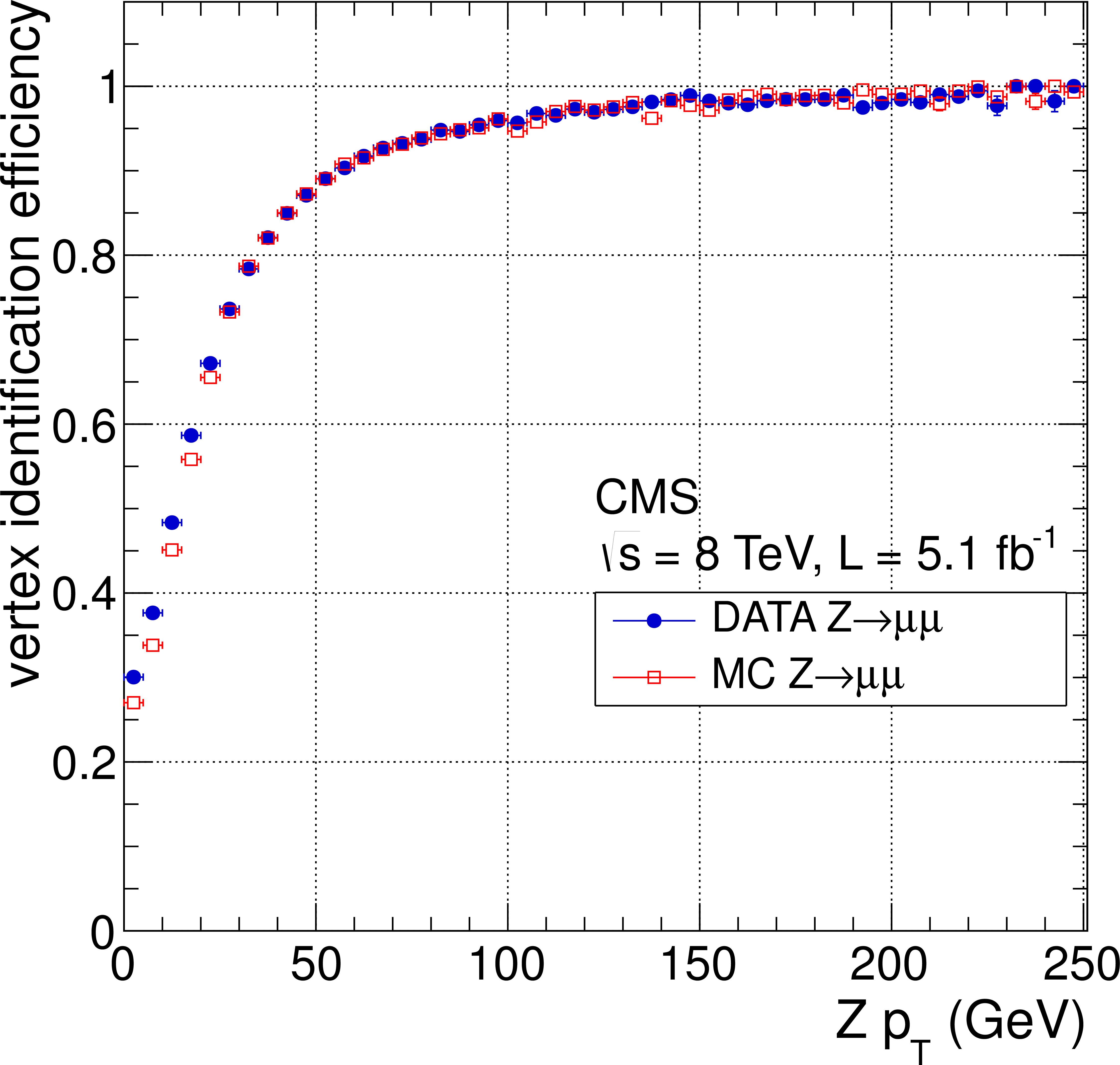
Figure 4:
Comparison of the vertex-identification efficiency between data (circles) and MC simulated $ {\mathrm {Z}} \to \mu \mu $ events (squares), as a function of the $Z$ boson $ {p_{\mathrm {T}}} $. |

png pdf |
Figure 5:
Comparison of the photon identification (ID) classifier variable distribution between 8 TeV data (points) and MC simulated events (histogram), separated into barrel (left) and endcap (right) electrons originating from $ {\mathrm {Z}}\to {\mathrm {e}} {\mathrm {e}}$ events. The uncertainties in the distributions from simulation are shown by the cross-hatched histogram. |
png pdf |
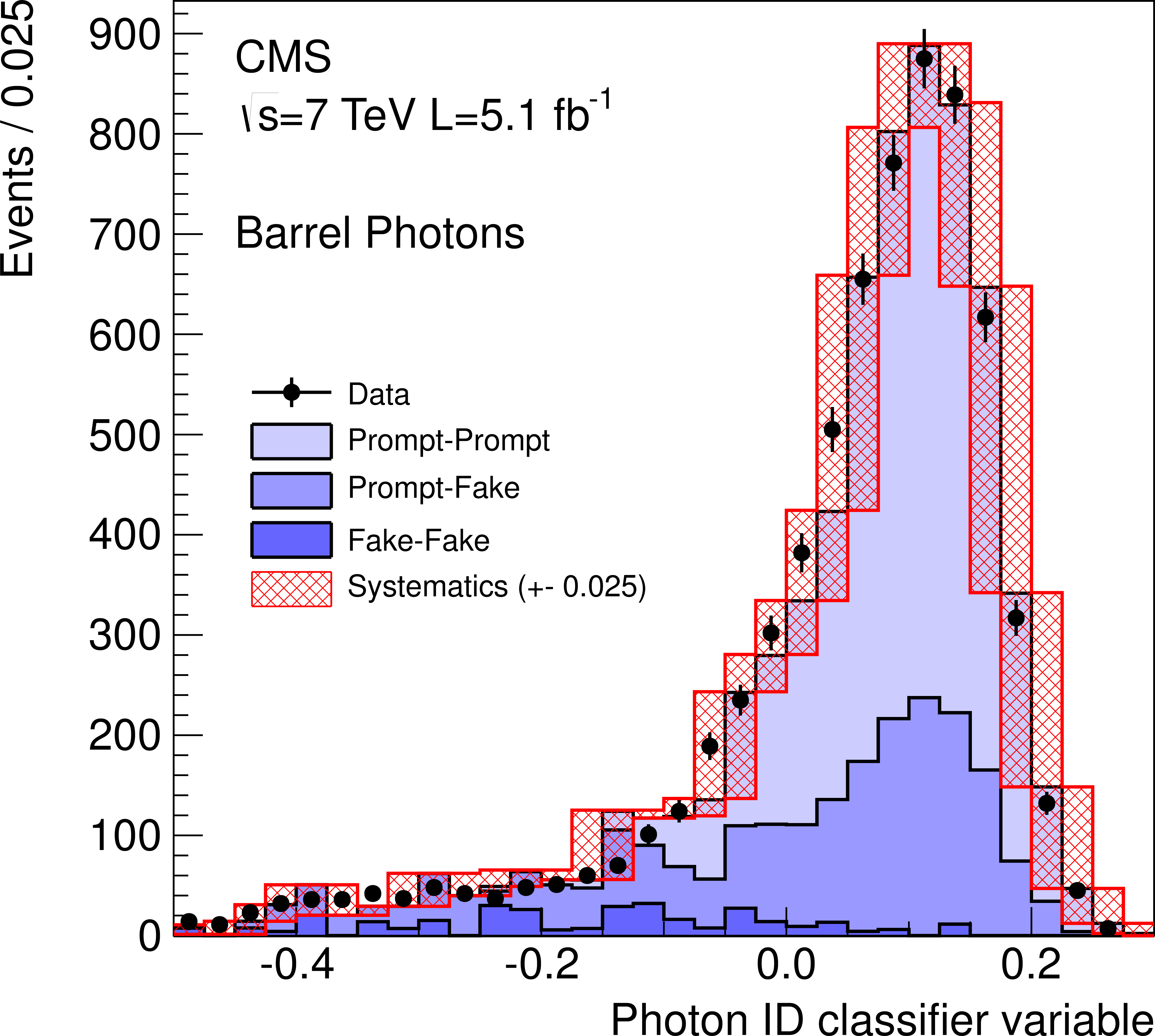
Figure 6-a:
Distribution of the photon ID classifier value for the larger transverse momentum photon in the ECAL barrel (left) and endcaps (right) from candidate diphoton data events (points) with $m_{\gamma \gamma }>$ 160 GeV. The predicted distributions for the various diphoton backgrounds as determined from simulation are shown by the histograms. The variations of the classifier value due to the systematic uncertainties are shown by the cross-hatched histogram. |

png pdf |
Figure 6-b:
Distribution of the photon ID classifier value for the larger transverse momentum photon in the ECAL barrel (left) and endcaps (right) from candidate diphoton data events (points) with $m_{\gamma \gamma }>$ 160 GeV. The predicted distributions for the various diphoton backgrounds as determined from simulation are shown by the histograms. The variations of the classifier value due to the systematic uncertainties are shown by the cross-hatched histogram. |

png pdf |
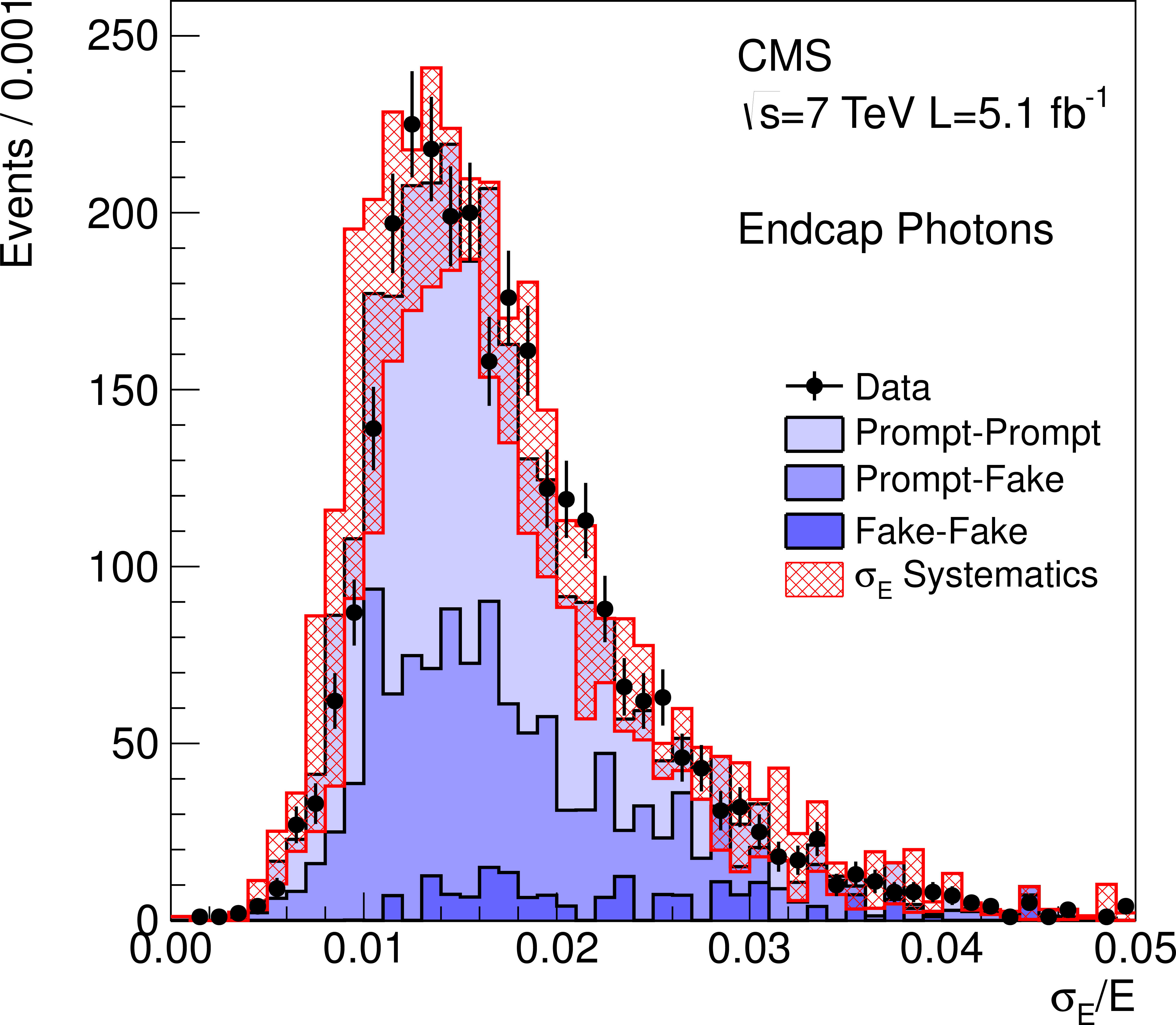
Figure 7-a:
Distribution of the photon resolution estimate $\sigma _E/E$ for the leading photon in the ECAL barrel (left) and endcaps (right) from candidate diphoton data events (points) with $m_{\gamma \gamma }>$ 160 GeV. The predicted distributions for the various diphoton backgrounds, as determined from simulation, are shown by the histograms. The variations of the resolution due to the systematic uncertainties are shown by the cross-hatched histogram. |
png pdf |
Figure 7-b:
Distribution of the photon resolution estimate $\sigma _E/E$ for the leading photon in the ECAL barrel (left) and endcaps (right) from candidate diphoton data events (points) with $m_{\gamma \gamma }>$ 160 GeV. The predicted distributions for the various diphoton backgrounds, as determined from simulation, are shown by the histograms. The variations of the resolution due to the systematic uncertainties are shown by the cross-hatched histogram. |

png pdf |
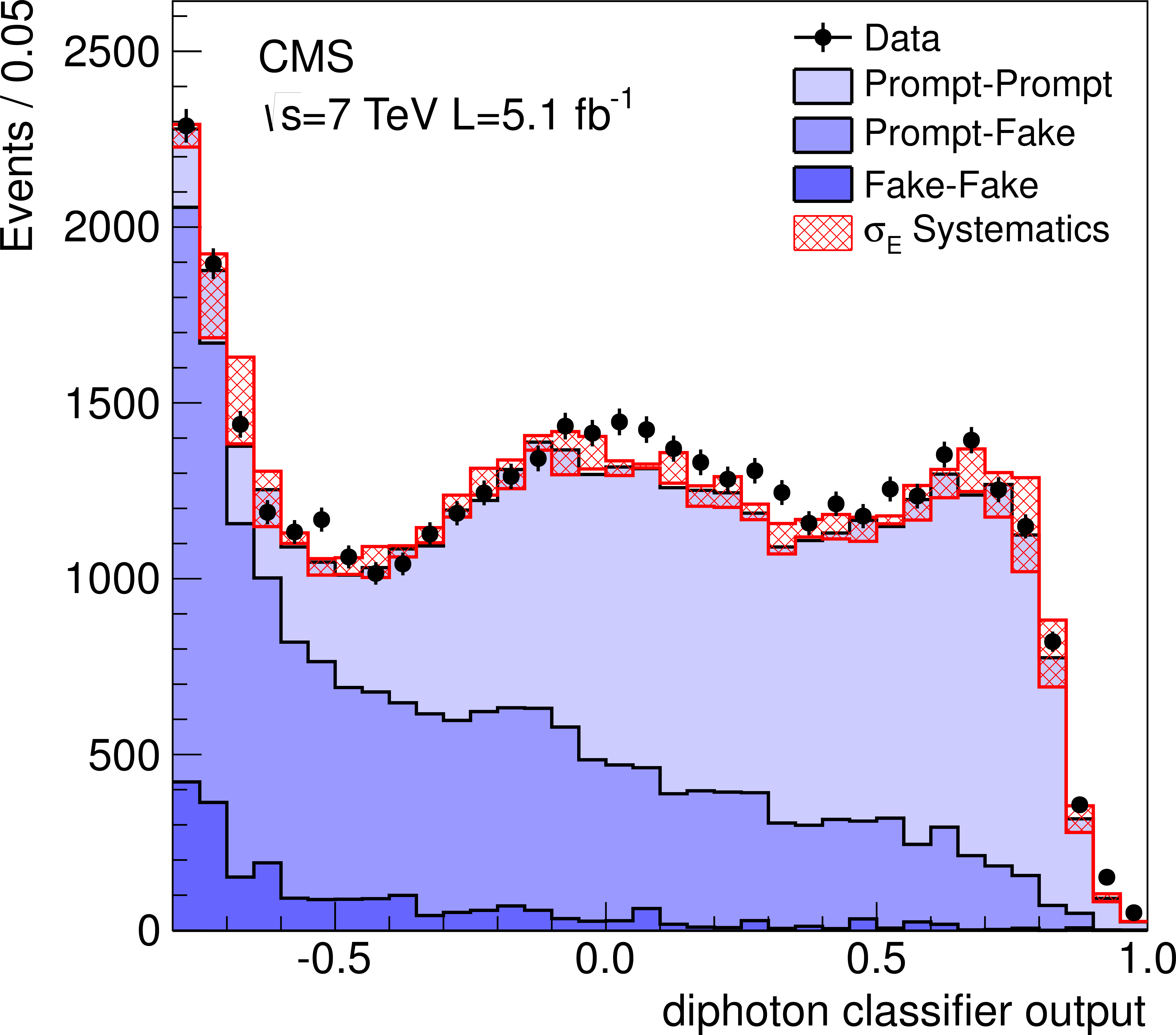
Figure 8-a:
The effect of the systematic uncertainty assigned to the photon identification classifier output (left) and the photon resolution estimate (right) on the diphoton BDT output for background MC simulation (100 GeV $< {m_{\gamma \gamma }} <$ 180 GeV ) and for data. The nominal BDT output is shown as a stacked histogram and the variation due to the uncertainty is shown as a cross-hatched band. These plots show only the systematic uncertainties that are common to both signal and background. There are additional significant uncertainties that are not shown here. |
png pdf |
Figure 8-b:
The effect of the systematic uncertainty assigned to the photon identification classifier output (left) and the photon resolution estimate (right) on the diphoton BDT output for background MC simulation (100 GeV $< {m_{\gamma \gamma }} <$ 180 GeV ) and for data. The nominal BDT output is shown as a stacked histogram and the variation due to the uncertainty is shown as a cross-hatched band. These plots show only the systematic uncertainties that are common to both signal and background. There are additional significant uncertainties that are not shown here. |
png pdf |
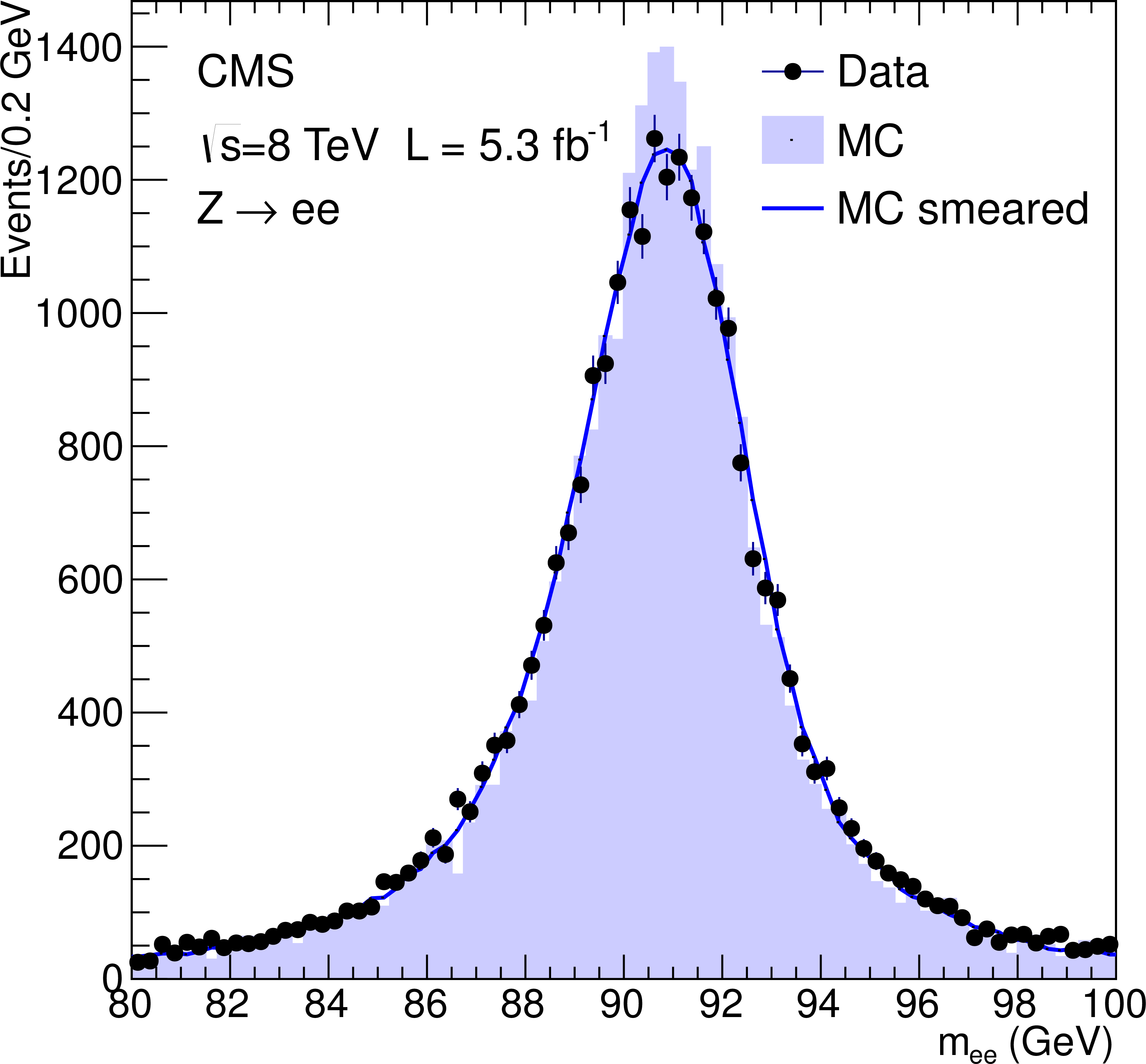
Figure 9:
Comparison of the dielectron invariant-mass spectrum from $ {\mathrm {Z}} \to {\mathrm {e}} {\mathrm {e}}$ events between 8 TeV data (points) and the simulated events (histogram), where the selected electrons are reconstructed as photons. The simulated distribution after applying smearing and scaling corrections of the electron energies is shown by the solid line. |
png pdf |
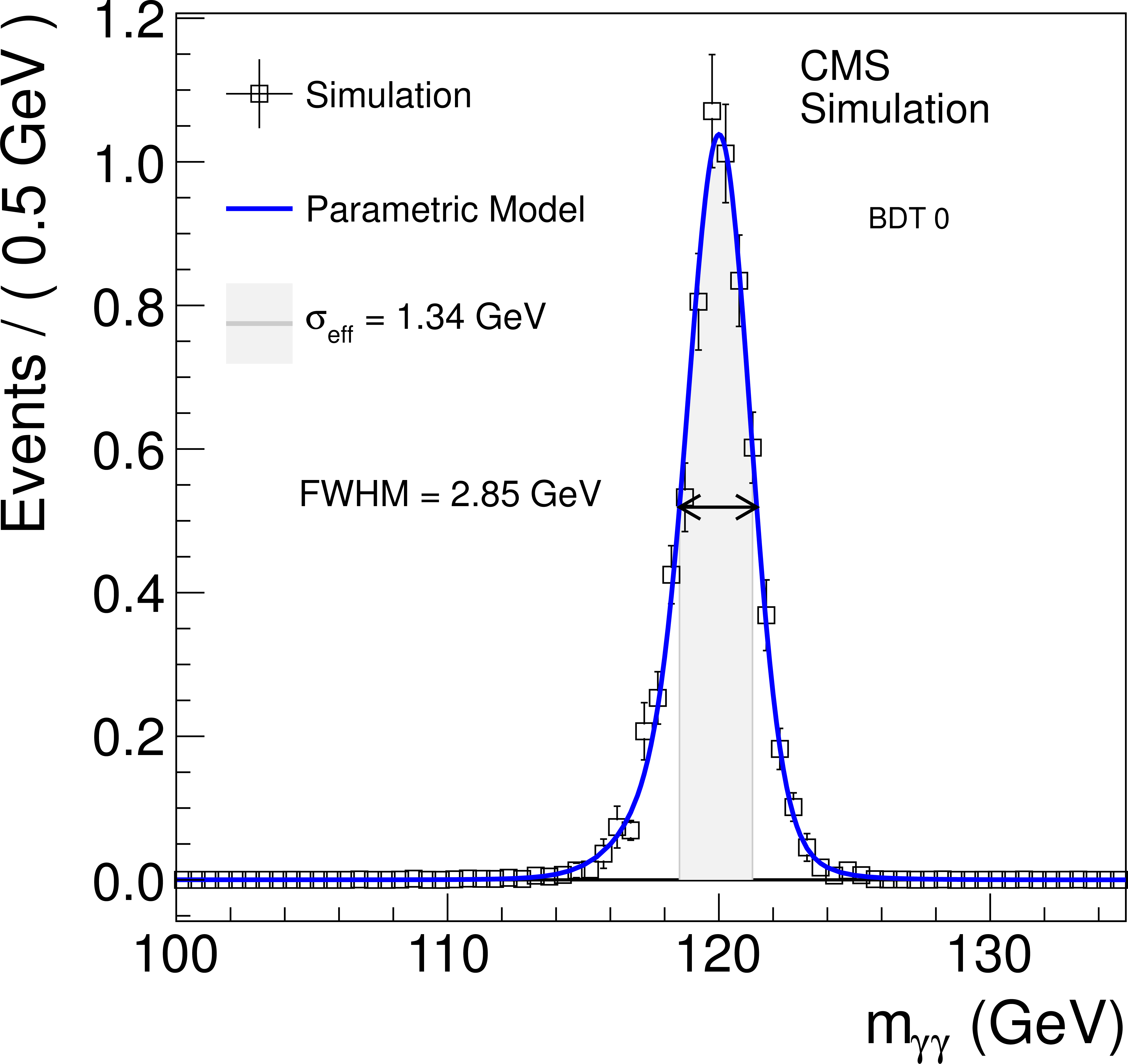
Figure 10-a:
Comparison of the diphoton invariant-mass distribution from the parametric signal model (blue line) and simulated MC events (open squares) for a Higgs mass hypothesis of $ {m_{ {\mathrm {H}} }}=$ 120 GeV for two (BDT 0 on the left, BDT 3 on the right) of the four 8 TeV BDT event classes. |
png pdf |
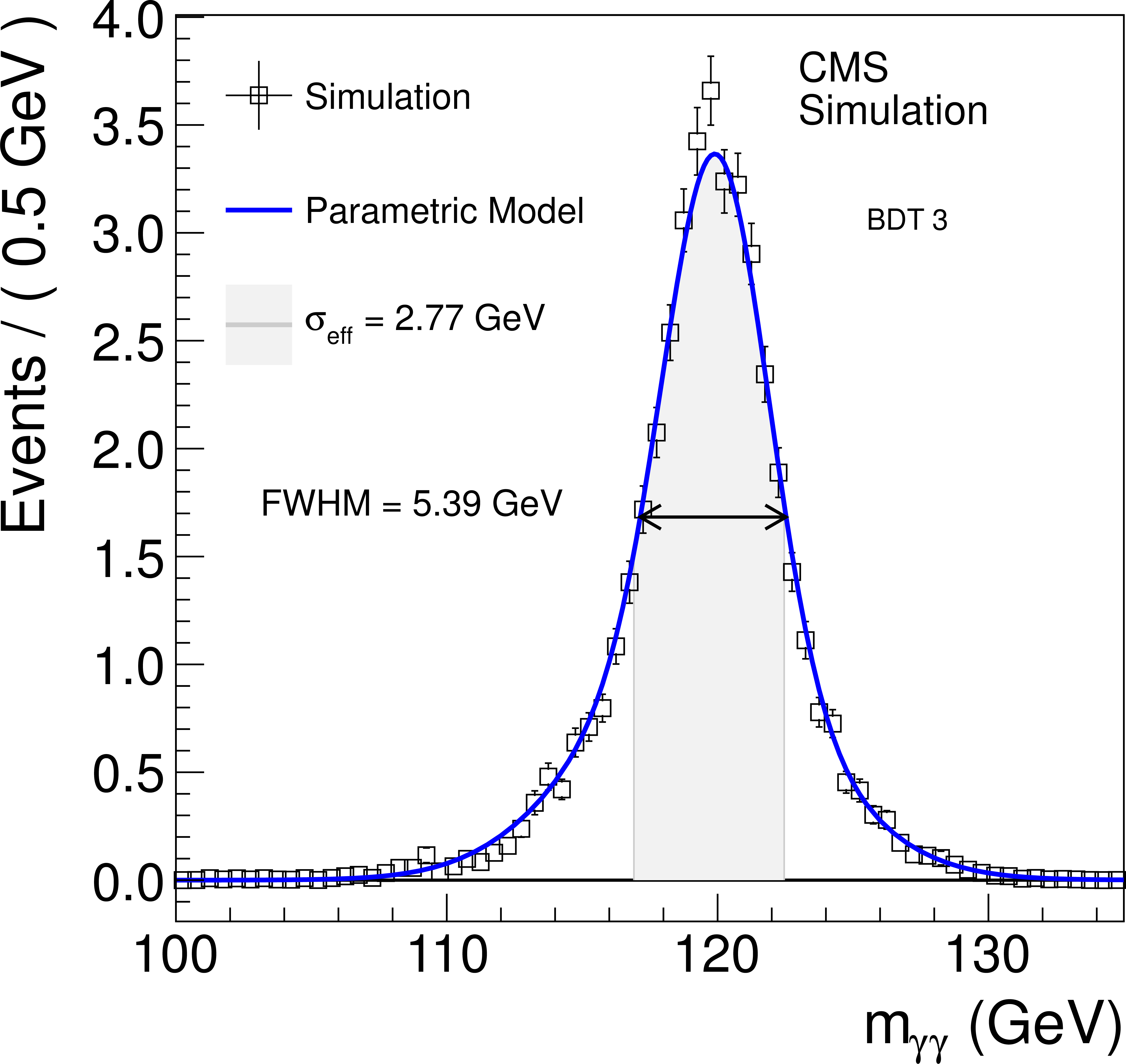
Figure 10-b:
Comparison of the diphoton invariant-mass distribution from the parametric signal model (blue line) and simulated MC events (open squares) for a Higgs mass hypothesis of $ {m_{ {\mathrm {H}} }}=$ 120 GeV for two (BDT 0 on the left, BDT 3 on the right) of the four 8 TeV BDT event classes. |
png pdf |
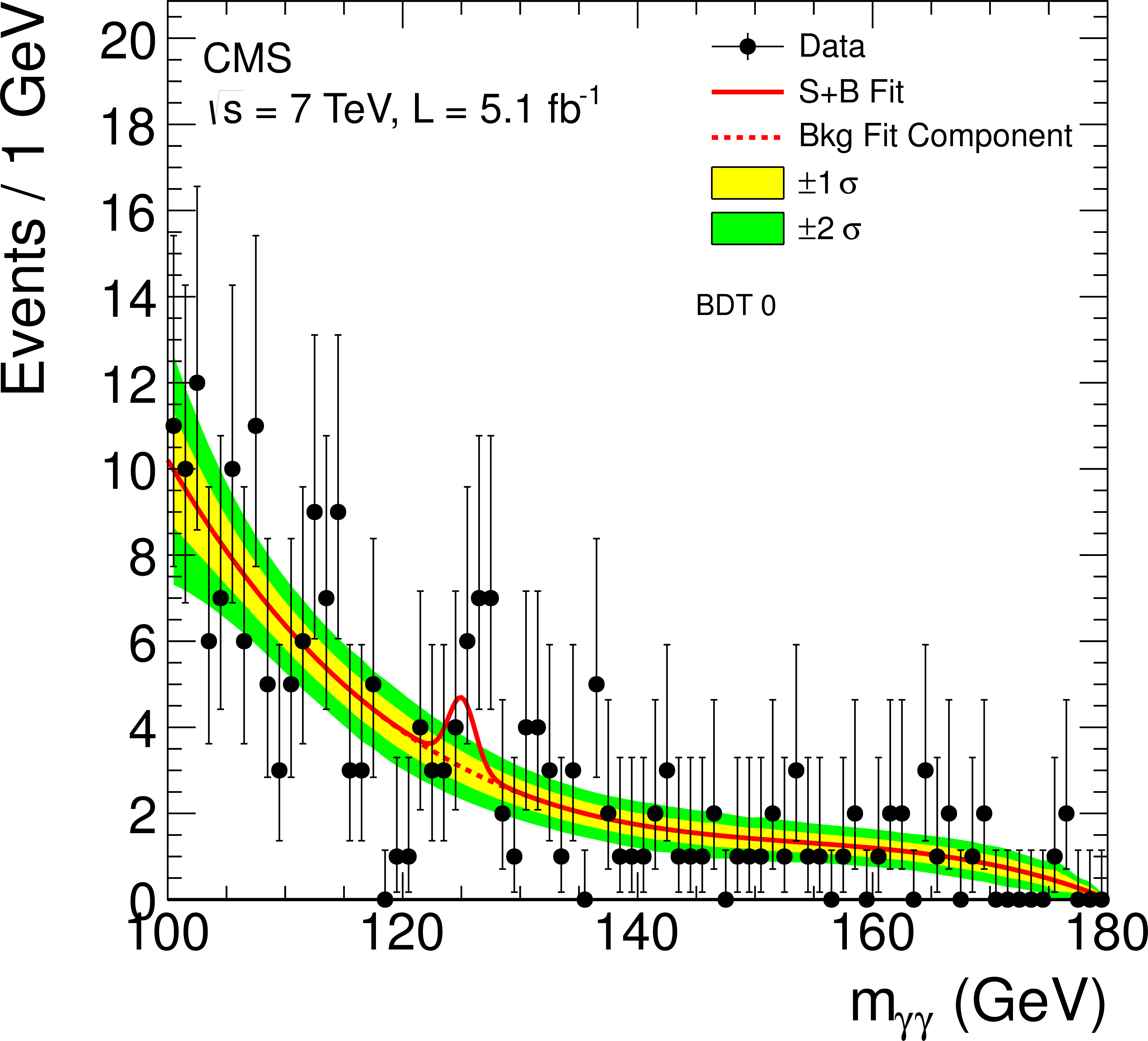
Figure 11-a:
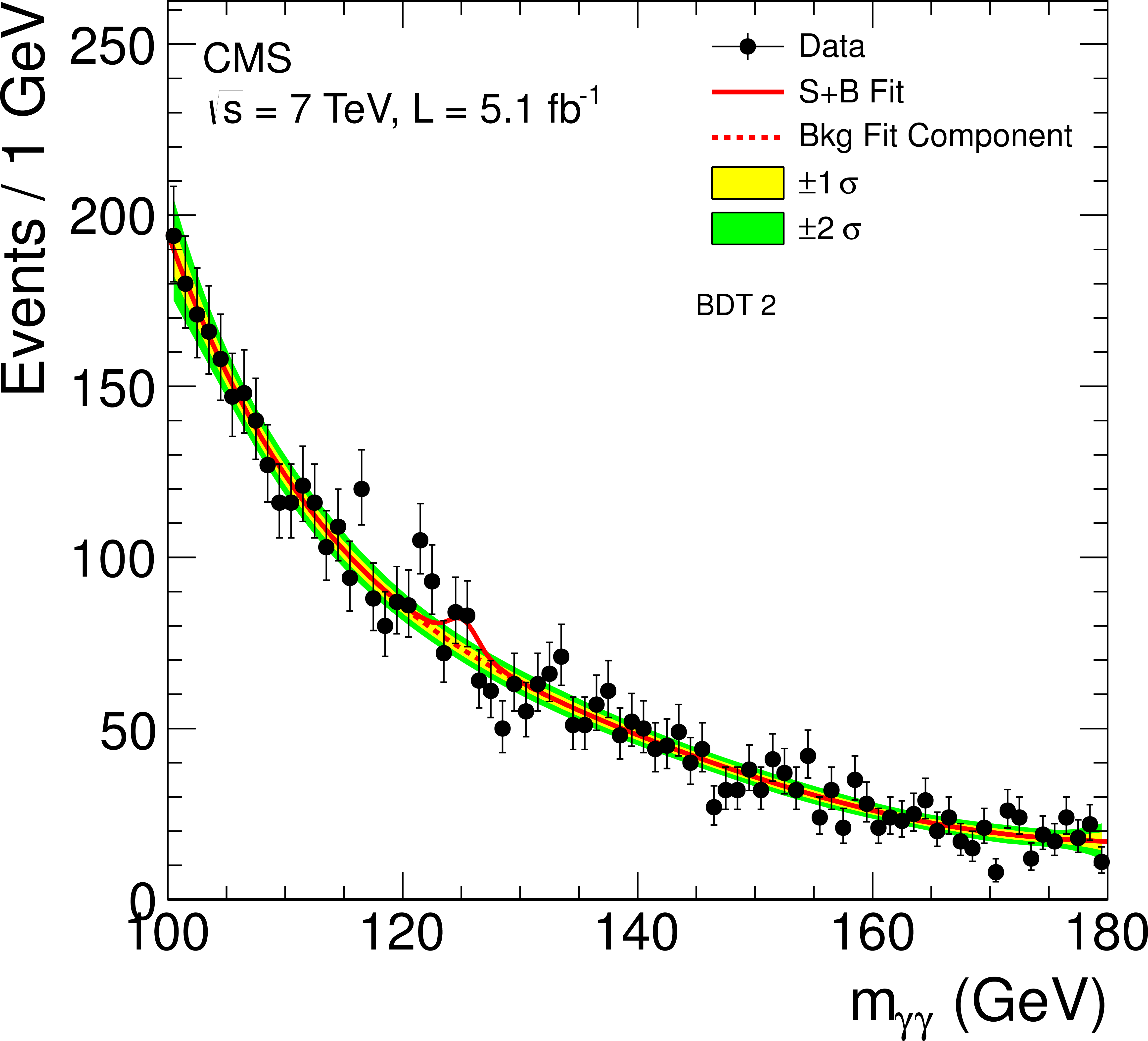
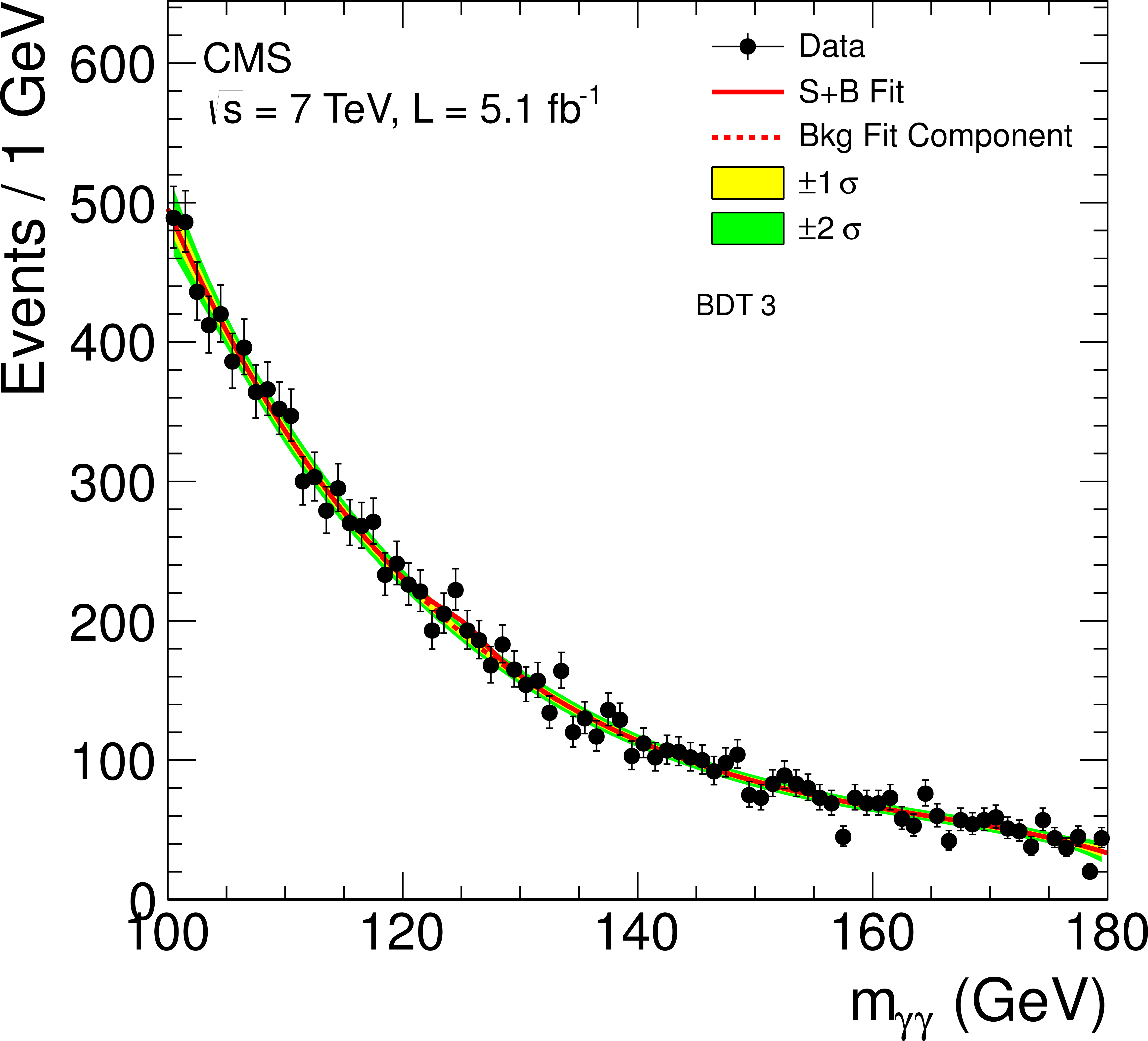
The diphoton invariant-mass distributions for the five classes of the 7 TeV data set (points) and the results of the signal-plus-background fits for $m_{\gamma \gamma }$ = 125 GeV (lines). The background fit components are shown by the dotted lines. The light and dark bands represent the ${\pm }$1 and ${\pm }$2 standard deviation uncertainties, respectively, on the background estimate. |
png pdf |
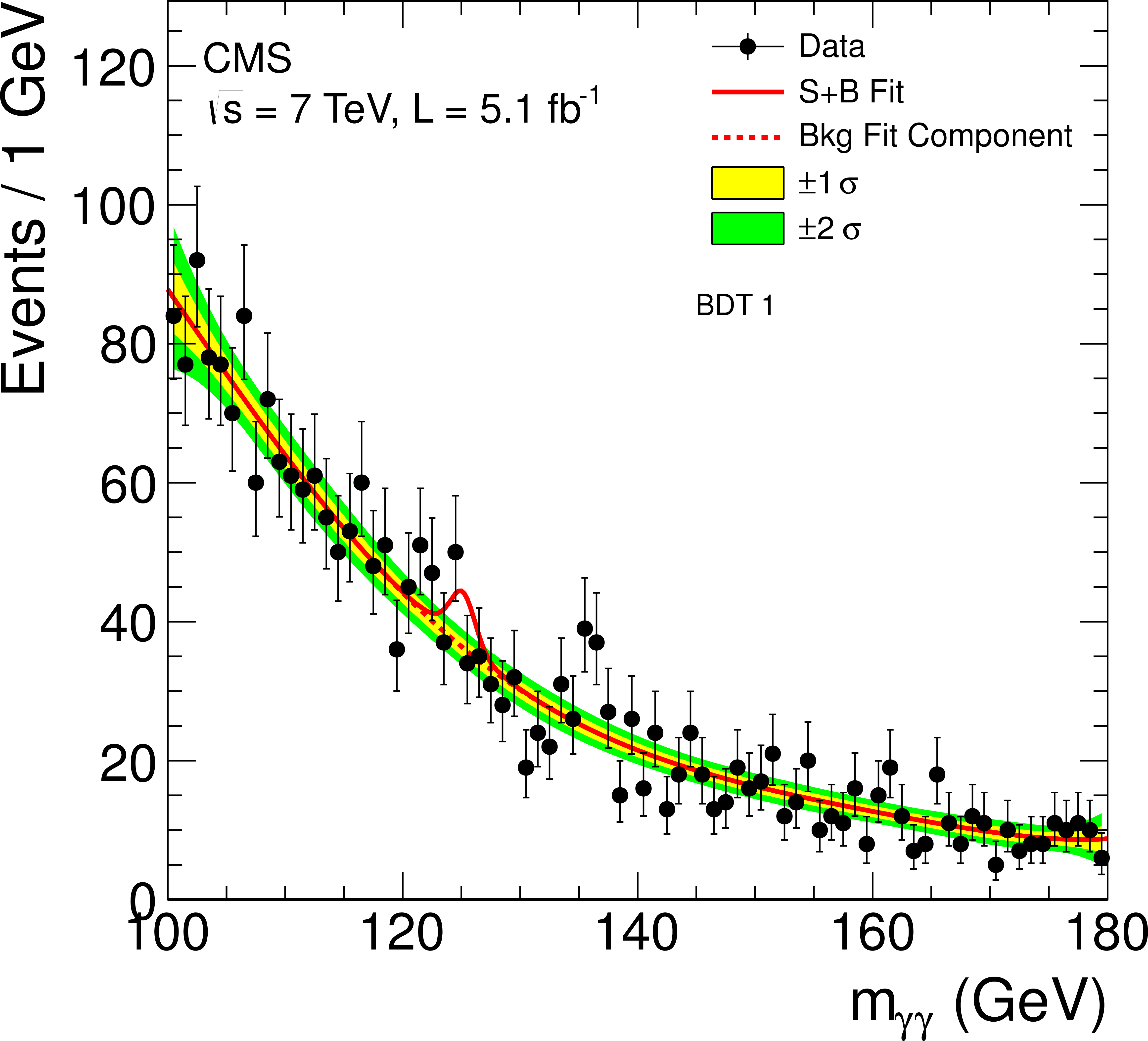
Figure 11-b:
The diphoton invariant-mass distributions for the five classes of the 7 TeV data set (points) and the results of the signal-plus-background fits for $m_{\gamma \gamma }$ = 125 GeV (lines). The background fit components are shown by the dotted lines. The light and dark bands represent the ${\pm }$1 and ${\pm }$2 standard deviation uncertainties, respectively, on the background estimate. |
png pdf |
Figure 11-c:
The diphoton invariant-mass distributions for the five classes of the 7 TeV data set (points) and the results of the signal-plus-background fits for $m_{\gamma \gamma }$ = 125 GeV (lines). The background fit components are shown by the dotted lines. The light and dark bands represent the ${\pm }$1 and ${\pm }$2 standard deviation uncertainties, respectively, on the background estimate. |
png pdf |
Figure 11-d:
The diphoton invariant-mass distributions for the five classes of the 7 TeV data set (points) and the results of the signal-plus-background fits for $m_{\gamma \gamma }$ = 125 GeV (lines). The background fit components are shown by the dotted lines. The light and dark bands represent the ${\pm }$1 and ${\pm }$2 standard deviation uncertainties, respectively, on the background estimate. |

png pdf |
Figure 11-e:
The diphoton invariant-mass distributions for the five classes of the 7 TeV data set (points) and the results of the signal-plus-background fits for $m_{\gamma \gamma }$ = 125 GeV (lines). The background fit components are shown by the dotted lines. The light and dark bands represent the ${\pm }$1 and ${\pm }$2 standard deviation uncertainties, respectively, on the background estimate. |
png pdf |
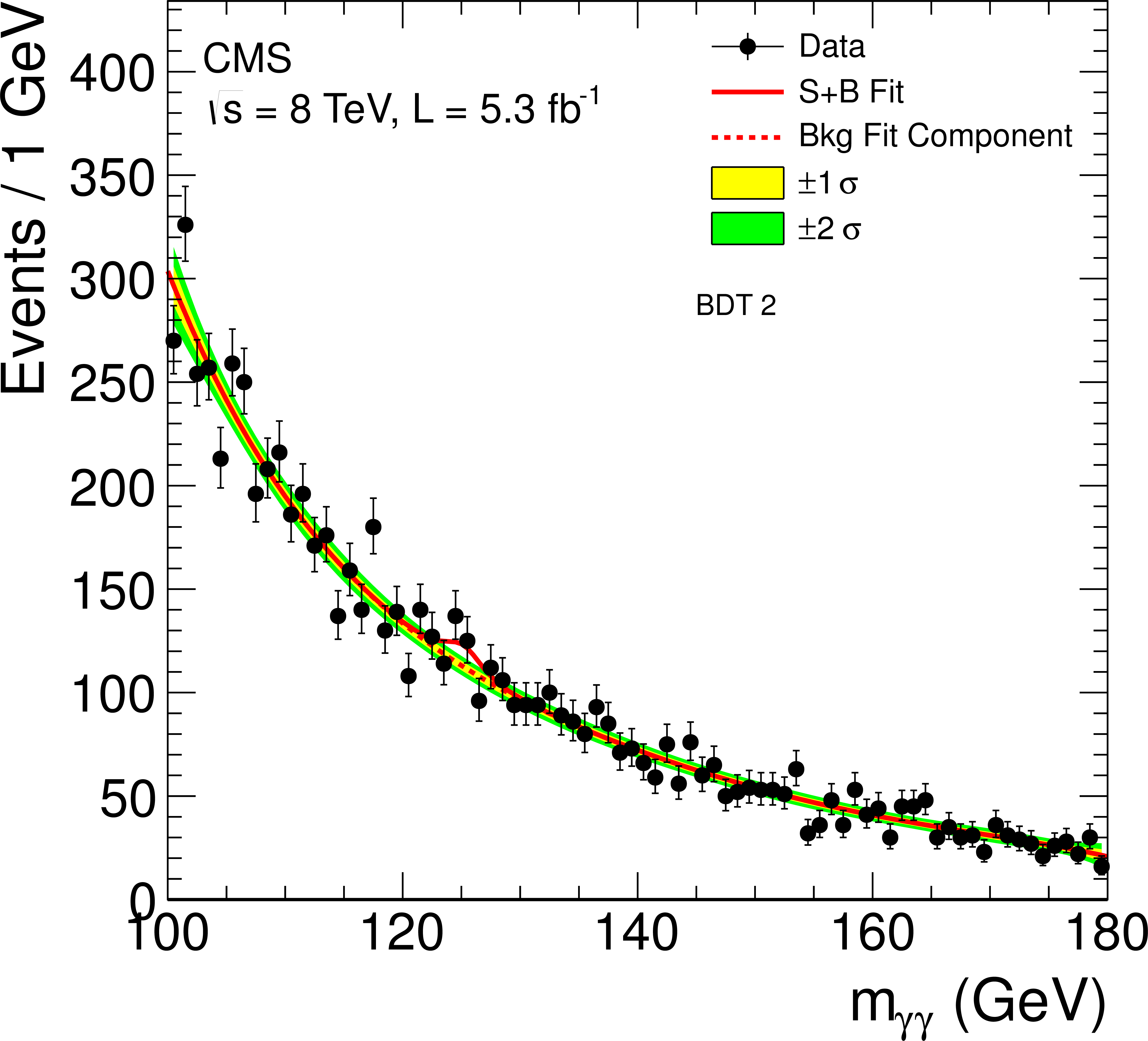
Figure 12-a:
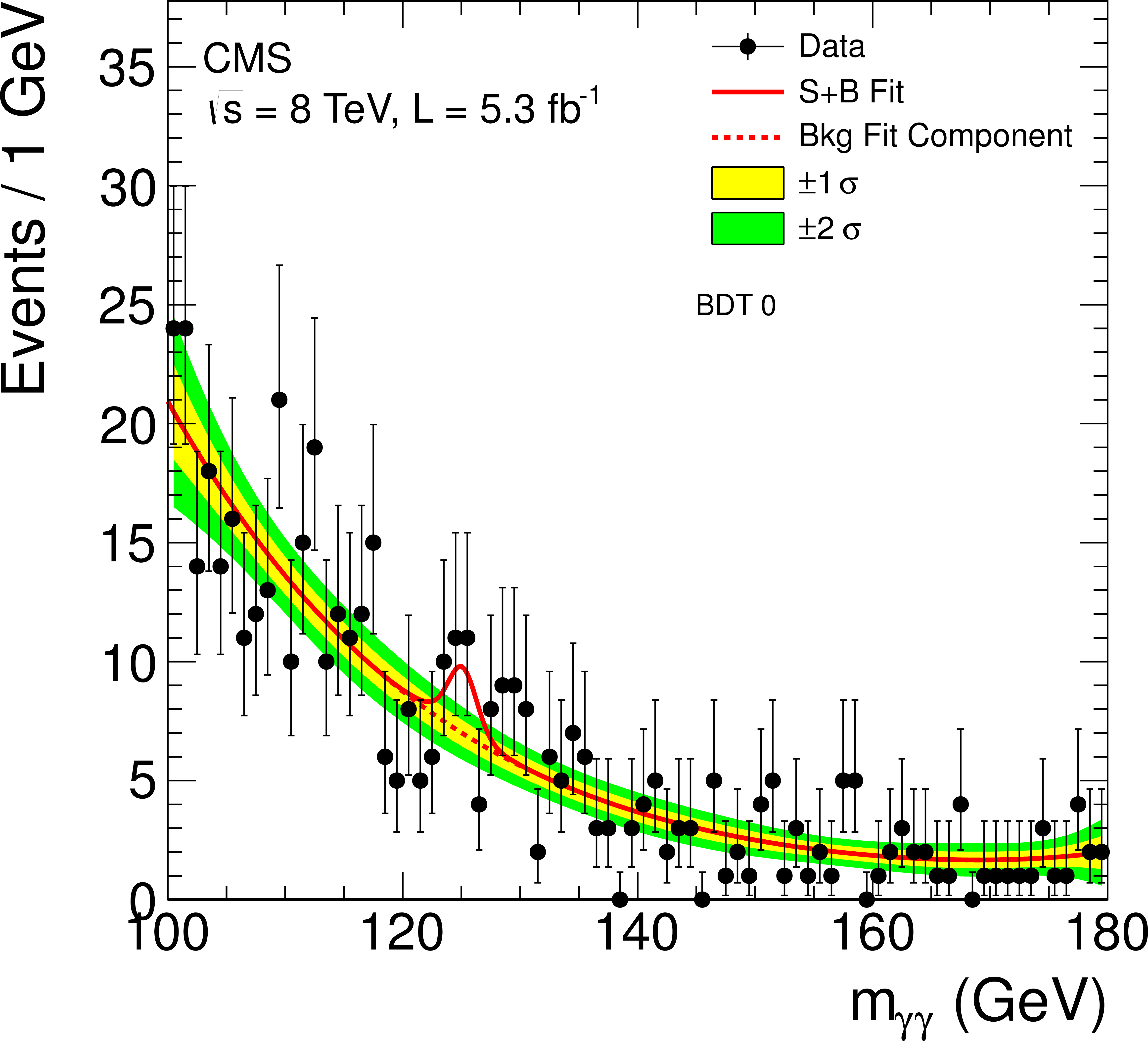
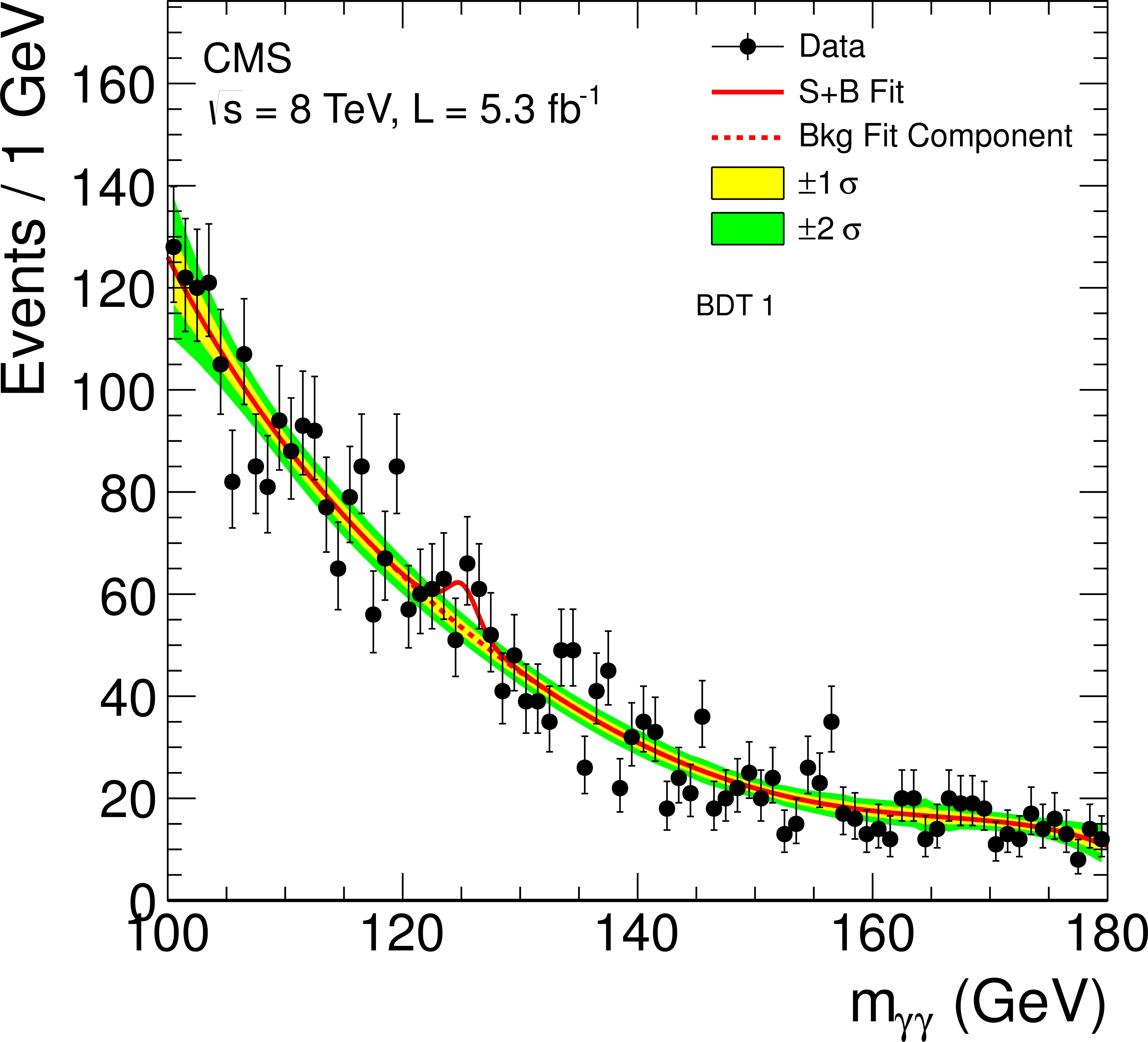
The diphoton invariant-mass distributions for the six classes of the 8 TeV data set (points) and the results of the signal-plus-background fits for $m_{\gamma \gamma }$ = 125 GeV (lines). The background fit components are shown by the dotted lines. The light and dark bands represent the ${\pm }$1 and ${\pm }$2 standard deviation uncertainties, respectively, on the background estimate. |
png pdf |
Figure 12-b:
The diphoton invariant-mass distributions for the six classes of the 8 TeV data set (points) and the results of the signal-plus-background fits for $m_{\gamma \gamma }$ = 125 GeV (lines). The background fit components are shown by the dotted lines. The light and dark bands represent the ${\pm }$1 and ${\pm }$2 standard deviation uncertainties, respectively, on the background estimate. |
png pdf |
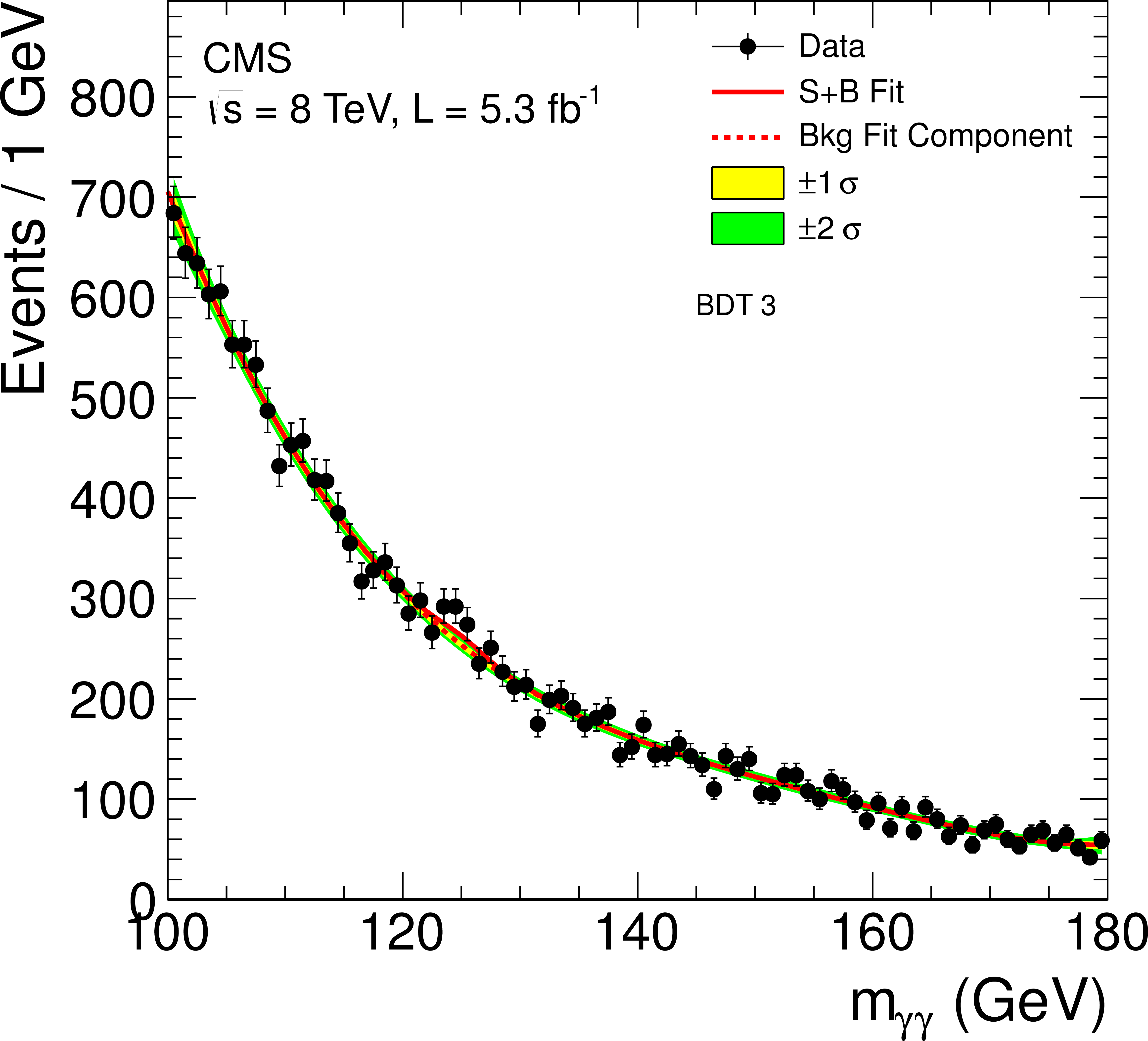
Figure 12-c:
The diphoton invariant-mass distributions for the six classes of the 8 TeV data set (points) and the results of the signal-plus-background fits for $m_{\gamma \gamma }$ = 125 GeV (lines). The background fit components are shown by the dotted lines. The light and dark bands represent the ${\pm }$1 and ${\pm }$2 standard deviation uncertainties, respectively, on the background estimate. |
png pdf |
Figure 12-d:
The diphoton invariant-mass distributions for the six classes of the 8 TeV data set (points) and the results of the signal-plus-background fits for $m_{\gamma \gamma }$ = 125 GeV (lines). The background fit components are shown by the dotted lines. The light and dark bands represent the ${\pm }$1 and ${\pm }$2 standard deviation uncertainties, respectively, on the background estimate. |
png pdf |
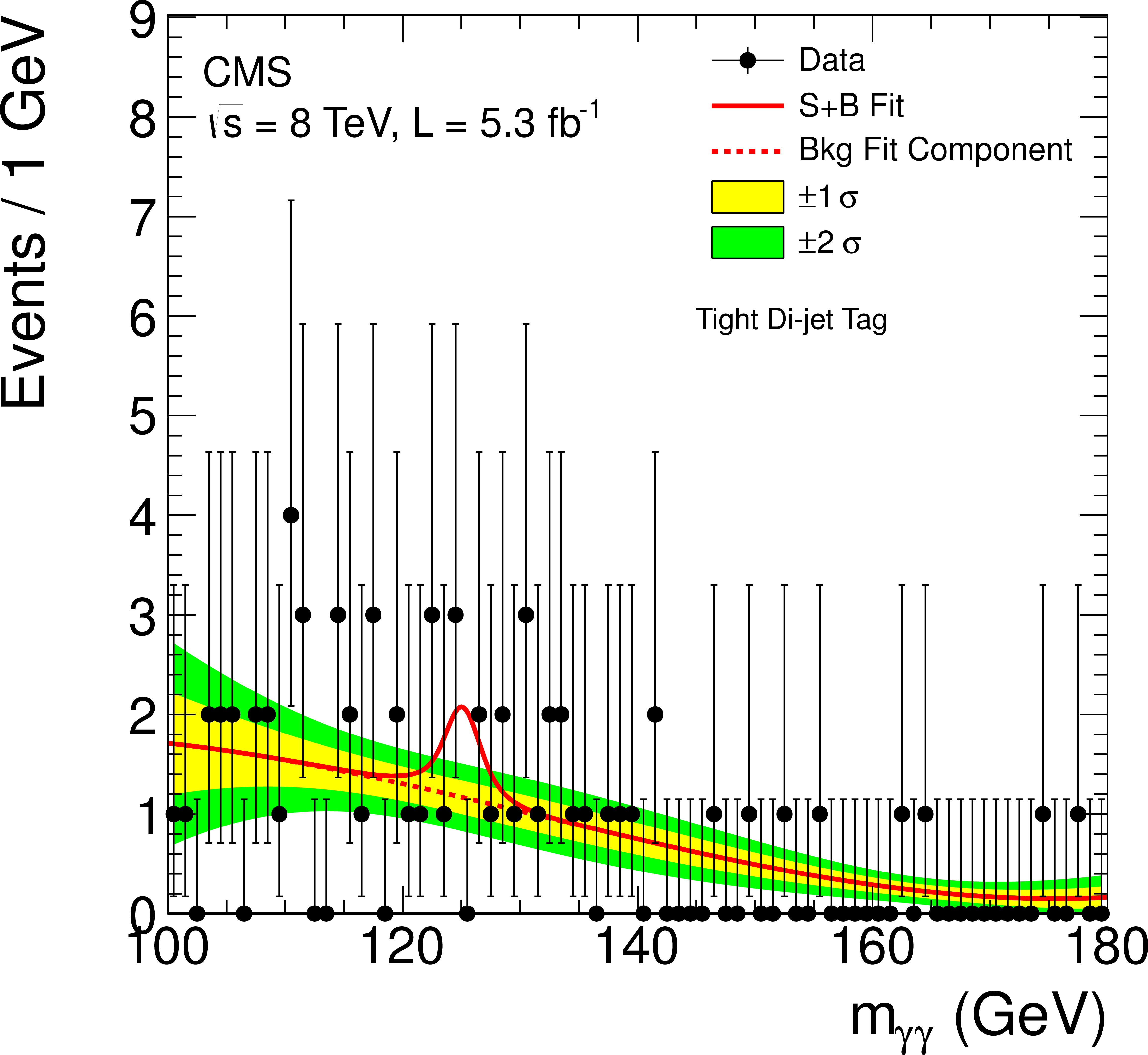
Figure 12-e:
The diphoton invariant-mass distributions for the six classes of the 8 TeV data set (points) and the results of the signal-plus-background fits for $m_{\gamma \gamma }$ = 125 GeV (lines). The background fit components are shown by the dotted lines. The light and dark bands represent the ${\pm }$1 and ${\pm }$2 standard deviation uncertainties, respectively, on the background estimate. |
png pdf |
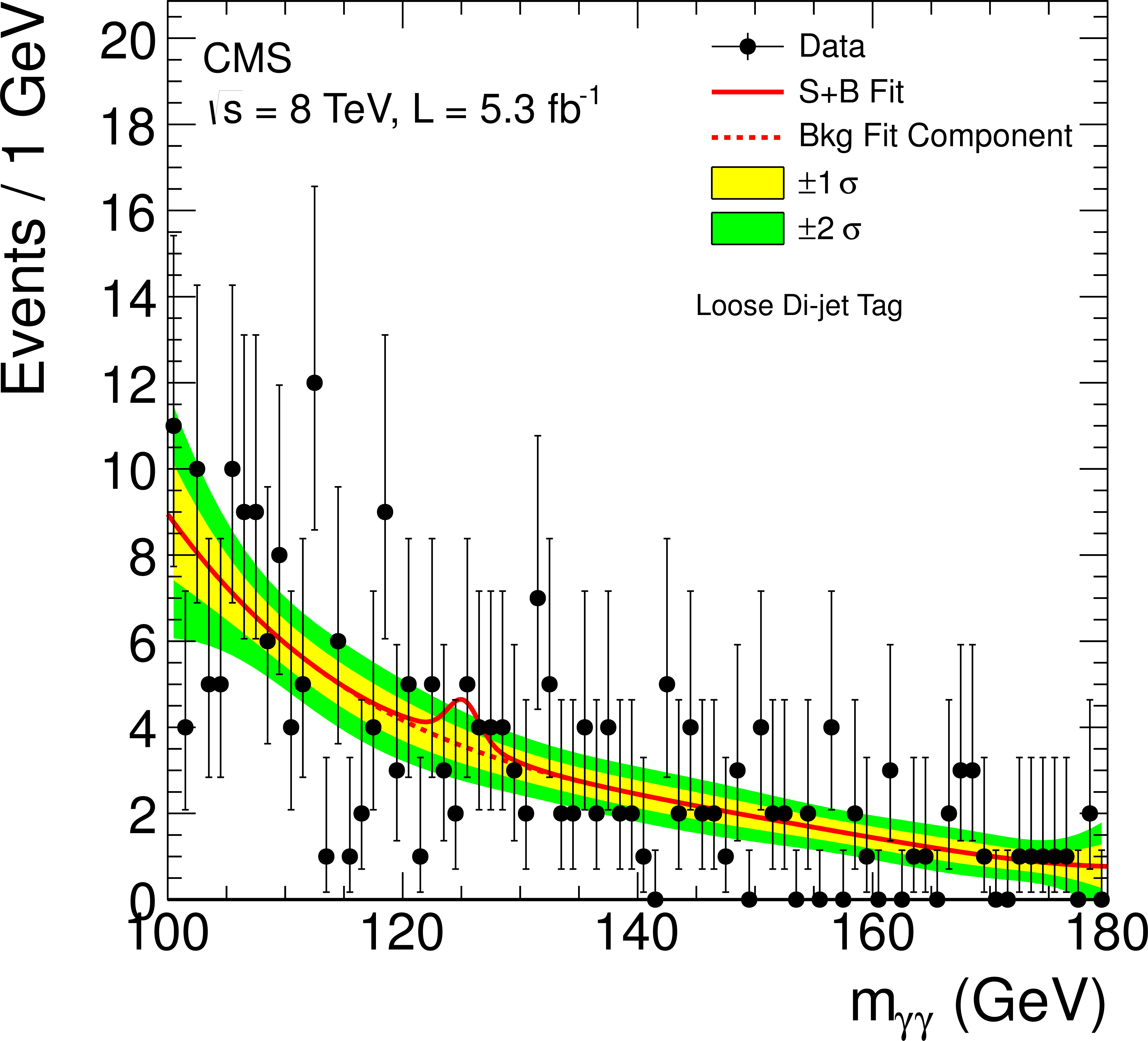
Figure 12-f:
The diphoton invariant-mass distributions for the six classes of the 8 TeV data set (points) and the results of the signal-plus-background fits for $m_{\gamma \gamma }$ = 125 GeV (lines). The background fit components are shown by the dotted lines. The light and dark bands represent the ${\pm }$1 and ${\pm }$2 standard deviation uncertainties, respectively, on the background estimate. |
png pdf |
Figure 13:
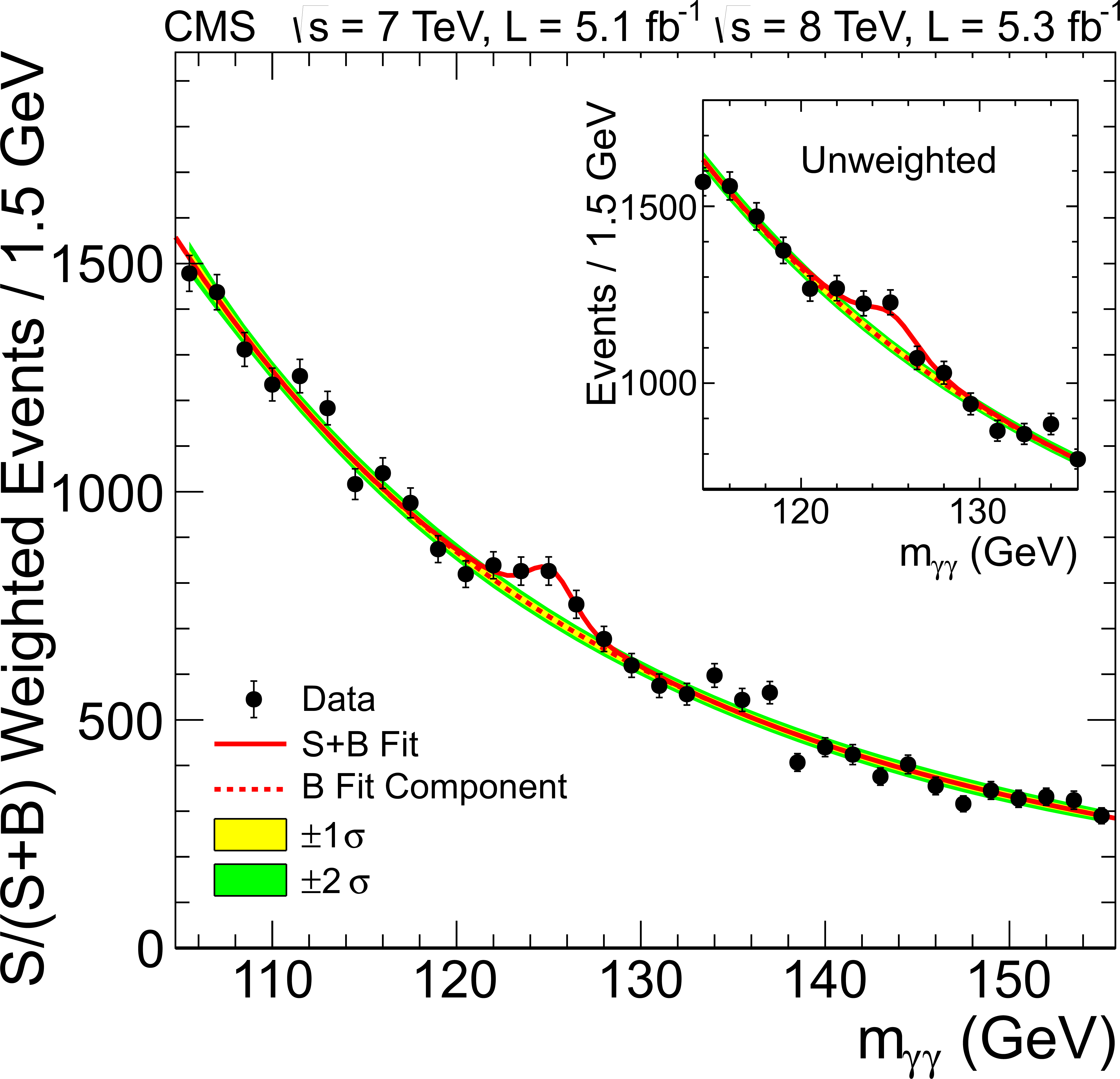
The diphoton invariant-mass distribution for the 7 and 8 TeV data sets (points), with each event weighted by the predicted $S/(S+B)$ ratio of its event class. The solid and dotted lines give the results of the signal-plus-background and background-only fit, respectively. The light and dark bands represent the $\pm $1 and $\pm $2 standard deviation uncertainties respectively on the background estimate. The inset shows the corresponding unweighted invariant-mass distribution around $m_{\gamma \gamma }$ = 125 GeV . |

png pdf |
Figure 14:
The six sidebands (dashed lines) around the signal region (solid line) in the sideband analysis. |

png pdf |
Figure 15-a:
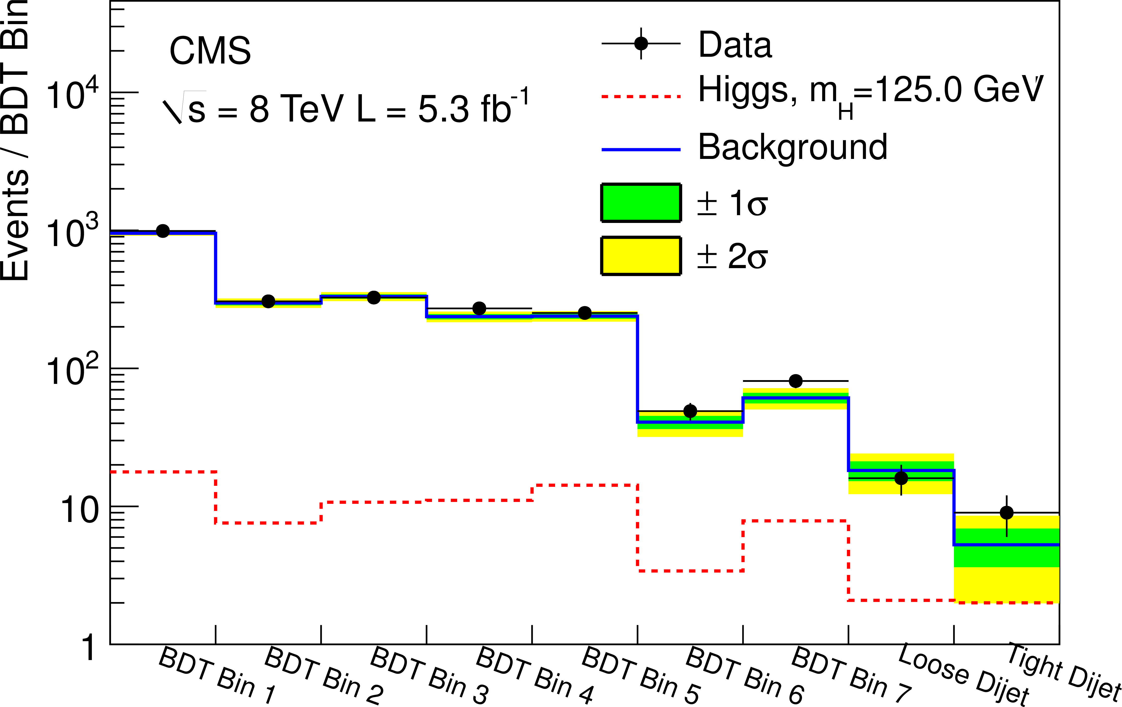
The number of observed events (points) for each of the mass-window BDT classes in the sideband analysis of $ {\mathrm {H}} \to \gamma \gamma $ for the 7 (left) and 8 TeV (right) data sets. The expected number of background events in each class, determined from the sidebands of the diphoton invariant-mass distribution, is shown by the solid line. The dark and light bands display the ${\pm }1$ and ${\pm }2$ standard deviation uncertainties in the background predictions, respectively. The expected number of signal events in each class for a 125 GeV Higgs boson, as determined from MC simulation, is shown by the dotted line. |
png pdf |
Figure 15-b:
The number of observed events (points) for each of the mass-window BDT classes in the sideband analysis of $ {\mathrm {H}} \to \gamma \gamma $ for the 7 (left) and 8 TeV (right) data sets. The expected number of background events in each class, determined from the sidebands of the diphoton invariant-mass distribution, is shown by the solid line. The dark and light bands display the ${\pm }1$ and ${\pm }2$ standard deviation uncertainties in the background predictions, respectively. The expected number of signal events in each class for a 125 GeV Higgs boson, as determined from MC simulation, is shown by the dotted line. |
png pdf |
Figure 16-a:
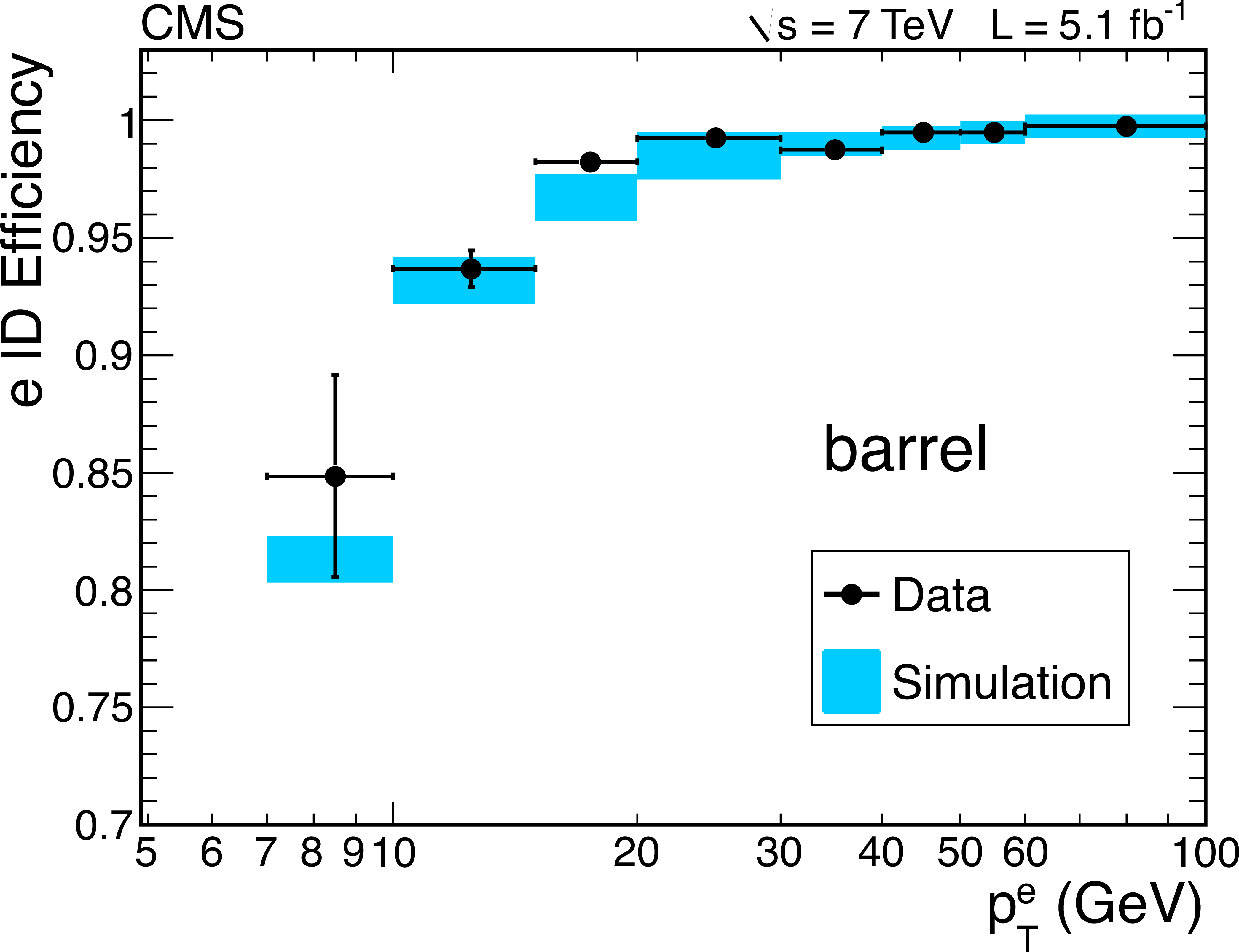
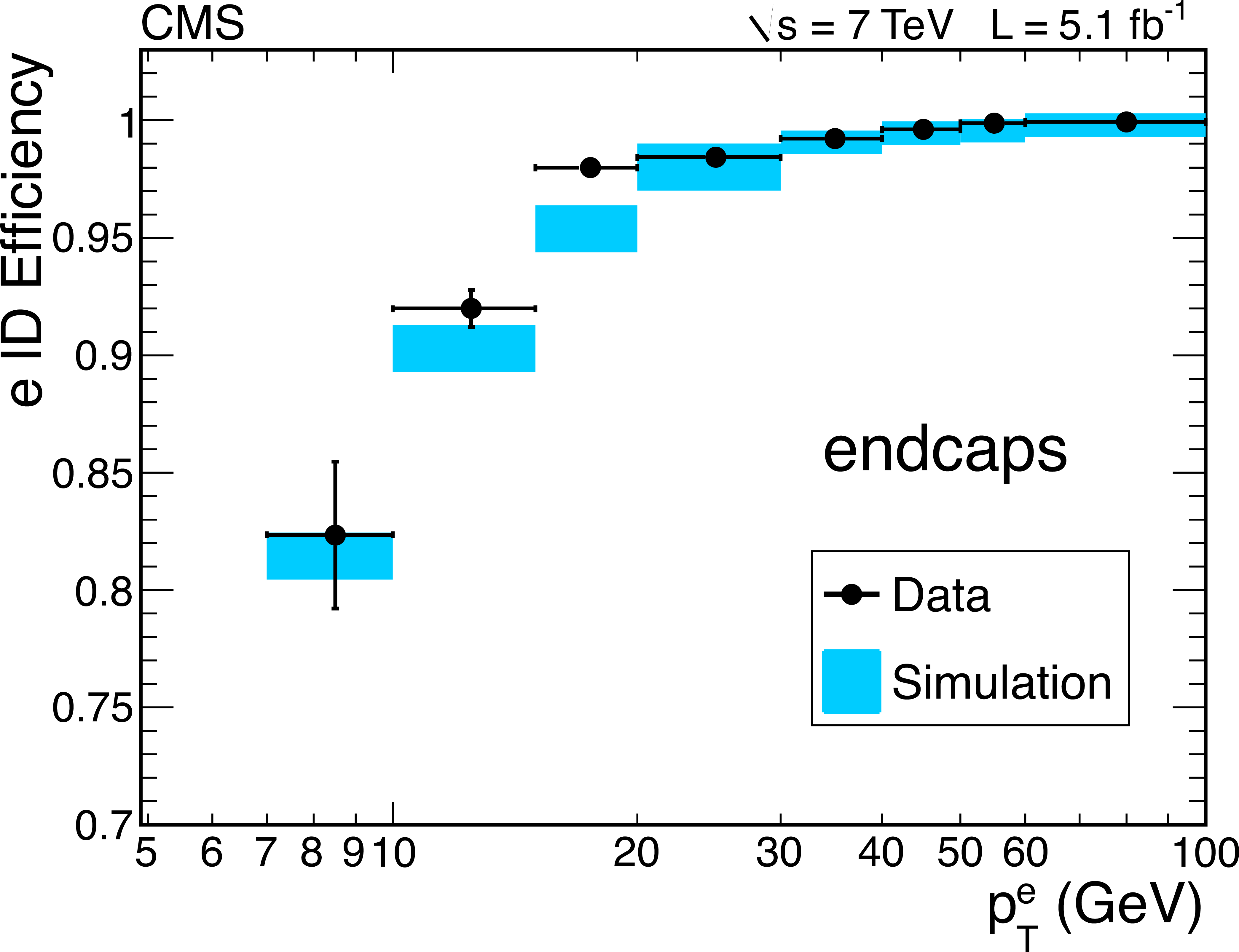
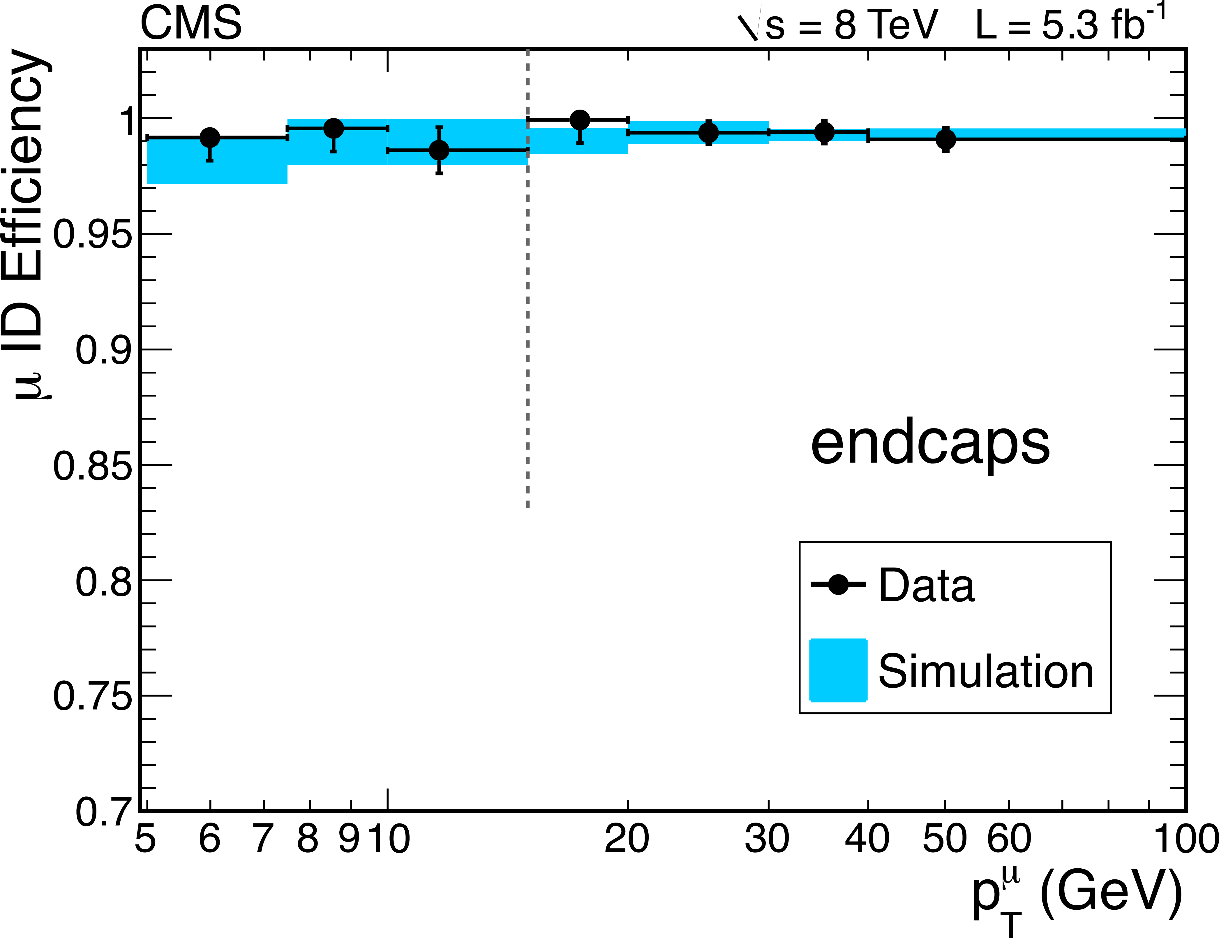
Measurements of the lepton identification efficiency using a tag-and-probe technique based on samples of Z and $ \mathrm{J}/\psi$ dilepton events. The measurements are shown for electrons (top) at 7 $ TeV $ and muons (bottom) at 8 $ TeV $ as a function of $ {p_{\mathrm {T}}} ^{\ell } $ for the $ |\eta | $ regions of the barrel (left) and endcaps (right). For muons, the efficiencies at $ {p_{\mathrm {T}}} ^{\mu } < $ 15 GeV (dashed line on bottom plots) is obtained using $ \mathrm{J}/\psi$. The results obtained from data (points with error bars) are compared to results obtained from MC simulation (histograms), with the shaded region representing the combined statistical and systematic uncertainties. |
png pdf |
Figure 16-b:
Measurements of the lepton identification efficiency using a tag-and-probe technique based on samples of Z and $ \mathrm{J}/\psi$ dilepton events. The measurements are shown for electrons (top) at 7 $ TeV $ and muons (bottom) at 8 $ TeV $ as a function of $ {p_{\mathrm {T}}} ^{\ell } $ for the $ |\eta | $ regions of the barrel (left) and endcaps (right). For muons, the efficiencies at $ {p_{\mathrm {T}}} ^{\mu } < $ 15 GeV (dashed line on bottom plots) is obtained using $ \mathrm{J}/\psi$. The results obtained from data (points with error bars) are compared to results obtained from MC simulation (histograms), with the shaded region representing the combined statistical and systematic uncertainties. |

png pdf |
Figure 16-c:
Measurements of the lepton identification efficiency using a tag-and-probe technique based on samples of Z and $ \mathrm{J}/\psi$ dilepton events. The measurements are shown for electrons (top) at 7 $ TeV $ and muons (bottom) at 8 $ TeV $ as a function of $ {p_{\mathrm {T}}} ^{\ell } $ for the $ |\eta | $ regions of the barrel (left) and endcaps (right). For muons, the efficiencies at $ {p_{\mathrm {T}}} ^{\mu } < $ 15 GeV (dashed line on bottom plots) is obtained using $ \mathrm{J}/\psi$. The results obtained from data (points with error bars) are compared to results obtained from MC simulation (histograms), with the shaded region representing the combined statistical and systematic uncertainties. |
png pdf |
Figure 16-d:
Measurements of the lepton identification efficiency using a tag-and-probe technique based on samples of Z and $ \mathrm{J}/\psi$ dilepton events. The measurements are shown for electrons (top) at 7 $ TeV $ and muons (bottom) at 8 $ TeV $ as a function of $ {p_{\mathrm {T}}} ^{\ell } $ for the $ |\eta | $ regions of the barrel (left) and endcaps (right). For muons, the efficiencies at $ {p_{\mathrm {T}}} ^{\mu } < $ 15 GeV (dashed line on bottom plots) is obtained using $ \mathrm{J}/\psi$. The results obtained from data (points with error bars) are compared to results obtained from MC simulation (histograms), with the shaded region representing the combined statistical and systematic uncertainties. |
png pdf |
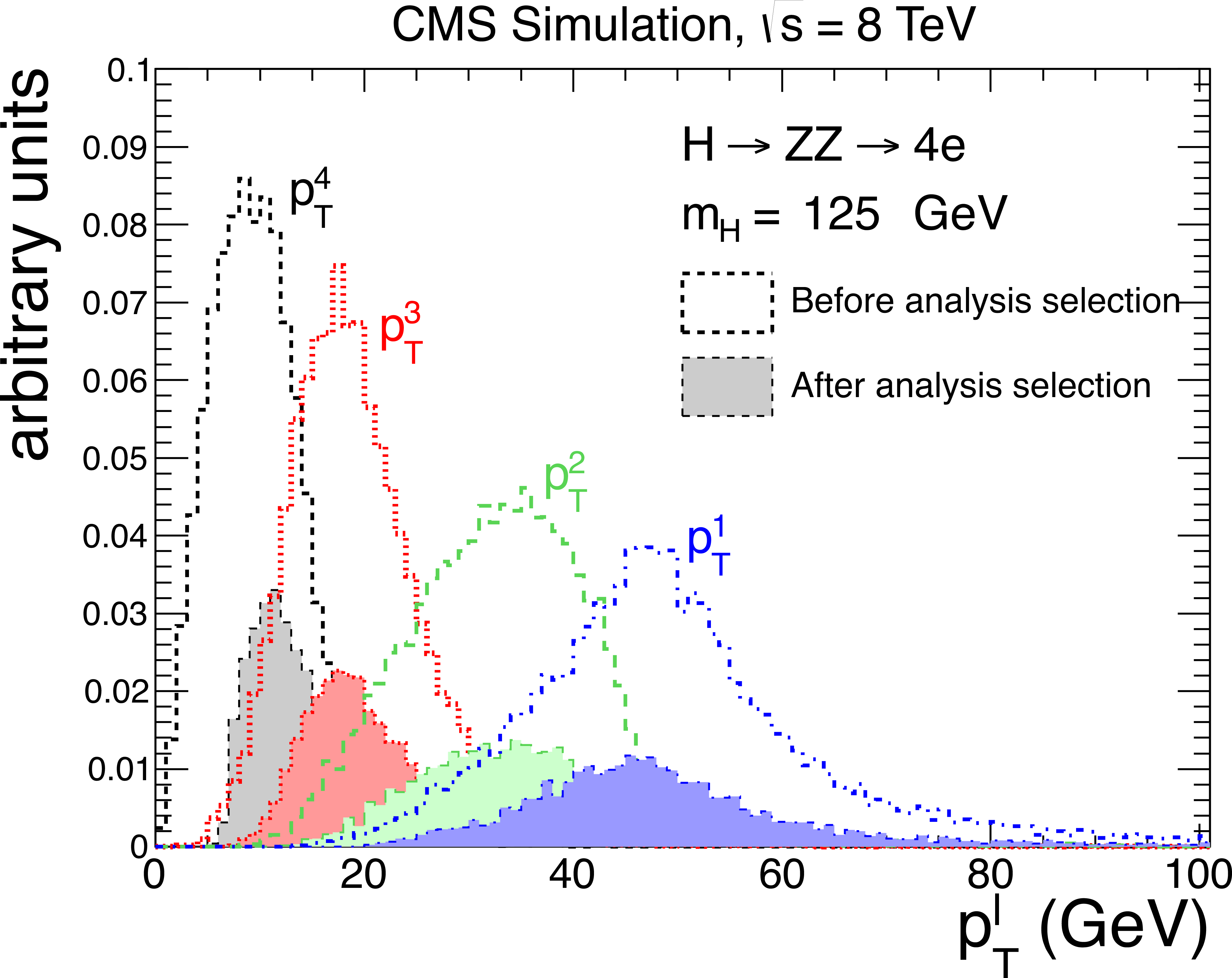
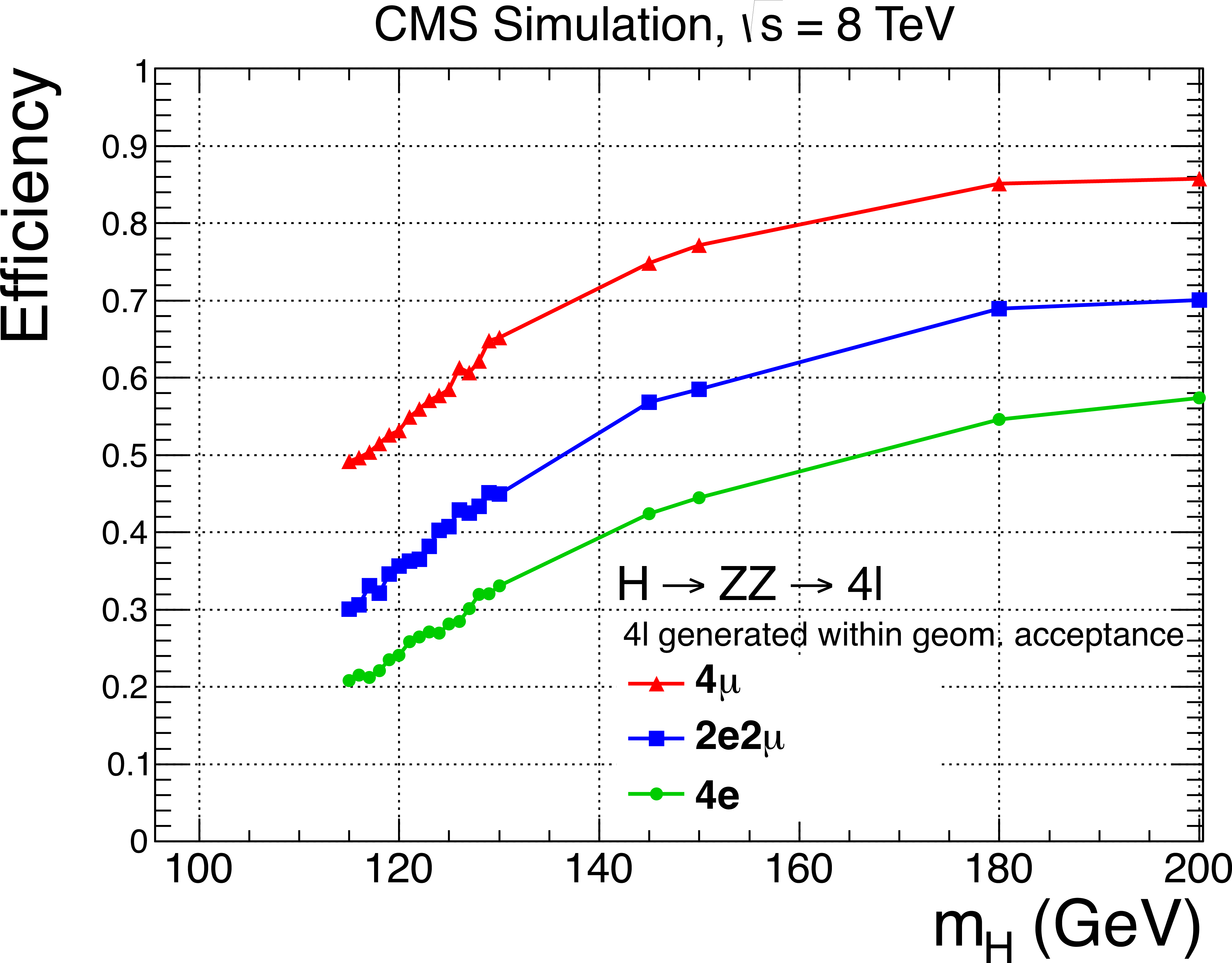
Figure 17-a:
The MC simulation distributions of the lepton transverse momentum $ {p_{\mathrm {T}}} ^{\ell }$ for each of the four leptons, ordered by $ {p_{\mathrm {T}}} ^{\ell }$, from the process $ {\mathrm {H}} \to {\mathrm {Z}} {\mathrm {Z}}\to 4\ell $ for a Higgs boson mass of 125 GeV in the $4 {\mathrm {e}}$ (top left), $4\mu $ (top right), and $2 {\mathrm {e}}2\mu $ (bottom left) channels. The distributions are shown for events when all four leptons are within the geometrical acceptance of the analysis (open histograms), and for events passing the final selection criteria (solid histograms).The bottom-right plot displays the event selection efficiencies for $ {\mathrm {H}} \to {\mathrm {Z}} {\mathrm {Z}}\to 4\ell $ determined from MC simulation, as a function of the Higgs boson mass, for the $4 {\mathrm {e}}$, $4\mu $, and $2 {\mathrm {e}}2\mu $ channels. The efficiencies are relative to events where all four leptons are within the geometrical acceptance. Divergent contributions from $ {\mathrm {Z}}\gamma ^*$ with $\gamma ^* \rightarrow \ell \ell $ at generator level are avoided by requiring that all dilepton invariant masses are greater than 1 GeV . |
png pdf |
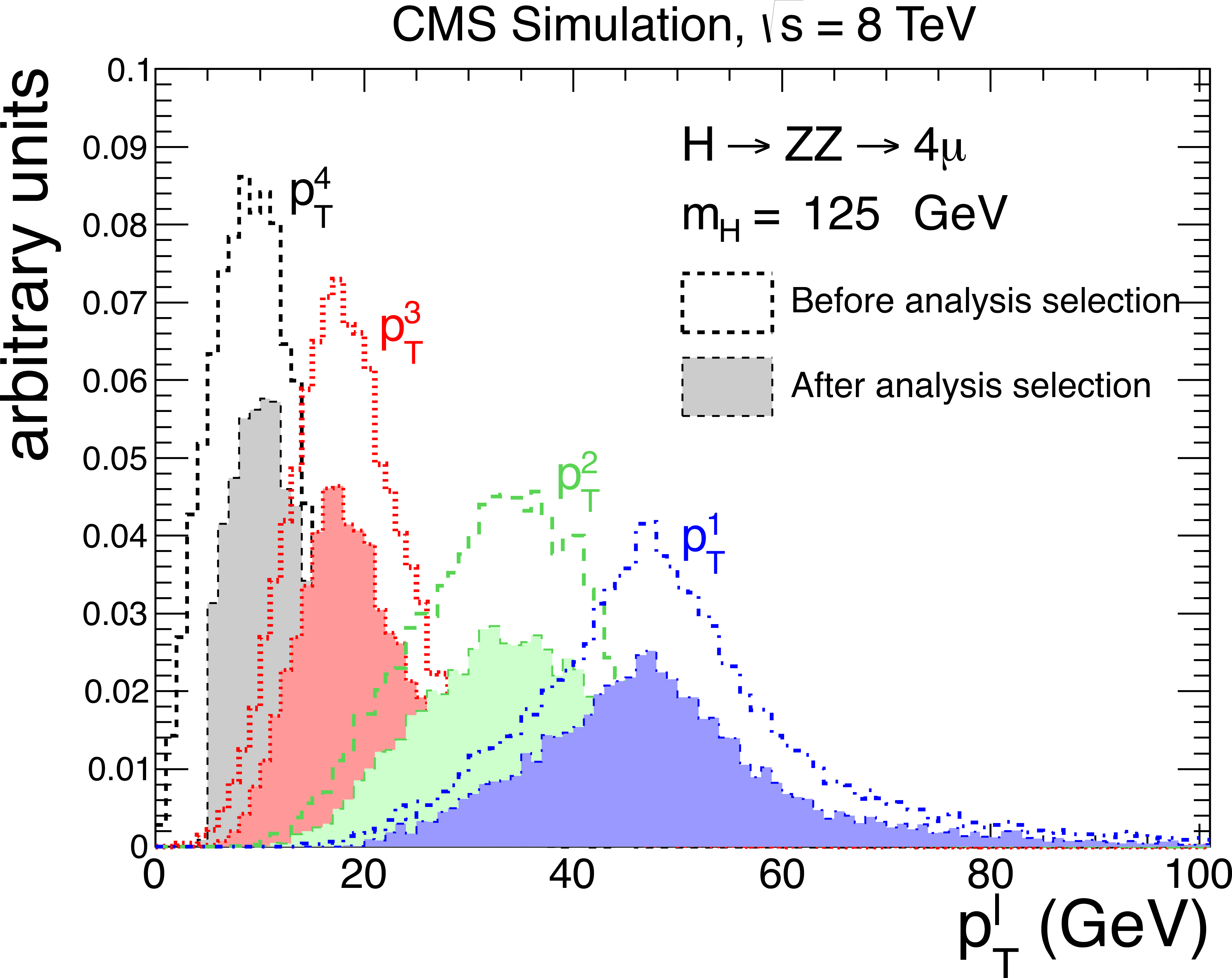
Figure 17-b:
The MC simulation distributions of the lepton transverse momentum $ {p_{\mathrm {T}}} ^{\ell }$ for each of the four leptons, ordered by $ {p_{\mathrm {T}}} ^{\ell }$, from the process $ {\mathrm {H}} \to {\mathrm {Z}} {\mathrm {Z}}\to 4\ell $ for a Higgs boson mass of 125 GeV in the $4 {\mathrm {e}}$ (top left), $4\mu $ (top right), and $2 {\mathrm {e}}2\mu $ (bottom left) channels. The distributions are shown for events when all four leptons are within the geometrical acceptance of the analysis (open histograms), and for events passing the final selection criteria (solid histograms).The bottom-right plot displays the event selection efficiencies for $ {\mathrm {H}} \to {\mathrm {Z}} {\mathrm {Z}}\to 4\ell $ determined from MC simulation, as a function of the Higgs boson mass, for the $4 {\mathrm {e}}$, $4\mu $, and $2 {\mathrm {e}}2\mu $ channels. The efficiencies are relative to events where all four leptons are within the geometrical acceptance. Divergent contributions from $ {\mathrm {Z}}\gamma ^*$ with $\gamma ^* \rightarrow \ell \ell $ at generator level are avoided by requiring that all dilepton invariant masses are greater than 1 GeV . |
png pdf |
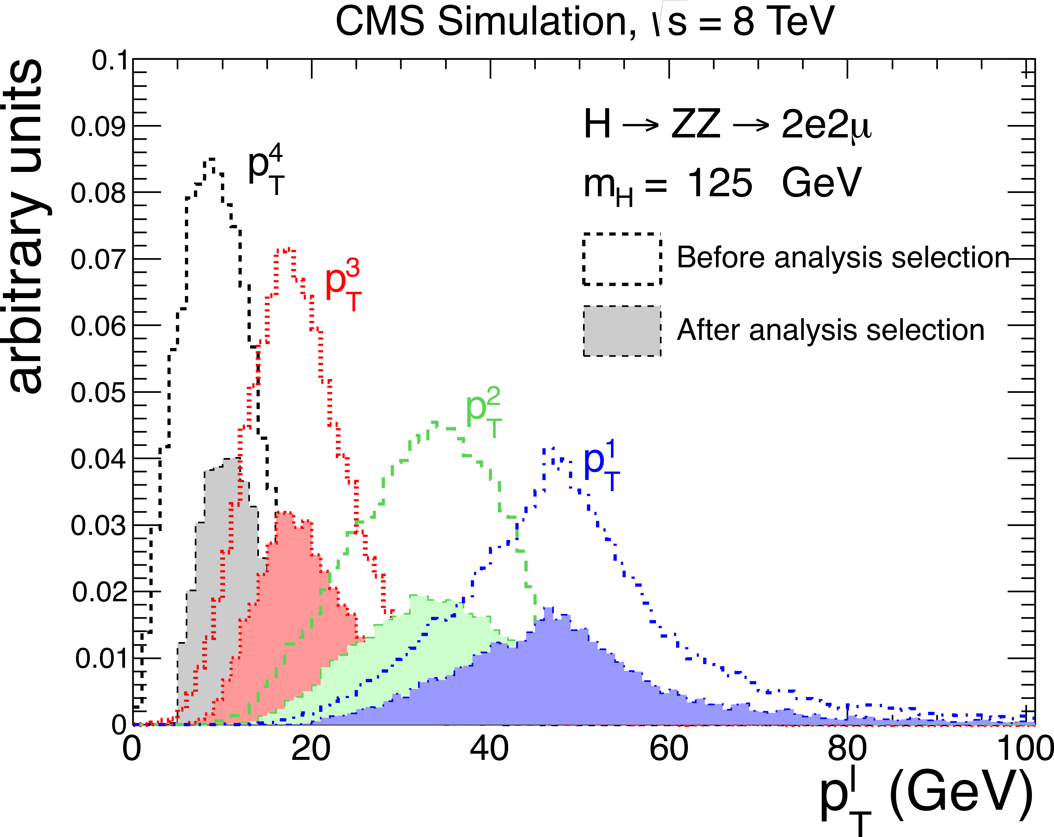
Figure 17-c:
The MC simulation distributions of the lepton transverse momentum $ {p_{\mathrm {T}}} ^{\ell }$ for each of the four leptons, ordered by $ {p_{\mathrm {T}}} ^{\ell }$, from the process $ {\mathrm {H}} \to {\mathrm {Z}} {\mathrm {Z}}\to 4\ell $ for a Higgs boson mass of 125 GeV in the $4 {\mathrm {e}}$ (top left), $4\mu $ (top right), and $2 {\mathrm {e}}2\mu $ (bottom left) channels. The distributions are shown for events when all four leptons are within the geometrical acceptance of the analysis (open histograms), and for events passing the final selection criteria (solid histograms).The bottom-right plot displays the event selection efficiencies for $ {\mathrm {H}} \to {\mathrm {Z}} {\mathrm {Z}}\to 4\ell $ determined from MC simulation, as a function of the Higgs boson mass, for the $4 {\mathrm {e}}$, $4\mu $, and $2 {\mathrm {e}}2\mu $ channels. The efficiencies are relative to events where all four leptons are within the geometrical acceptance. Divergent contributions from $ {\mathrm {Z}}\gamma ^*$ with $\gamma ^* \rightarrow \ell \ell $ at generator level are avoided by requiring that all dilepton invariant masses are greater than 1 GeV . |
png pdf |
Figure 17-d:
The MC simulation distributions of the lepton transverse momentum $ {p_{\mathrm {T}}} ^{\ell }$ for each of the four leptons, ordered by $ {p_{\mathrm {T}}} ^{\ell }$, from the process $ {\mathrm {H}} \to {\mathrm {Z}} {\mathrm {Z}}\to 4\ell $ for a Higgs boson mass of 125 GeV in the $4 {\mathrm {e}}$ (top left), $4\mu $ (top right), and $2 {\mathrm {e}}2\mu $ (bottom left) channels. The distributions are shown for events when all four leptons are within the geometrical acceptance of the analysis (open histograms), and for events passing the final selection criteria (solid histograms).The bottom-right plot displays the event selection efficiencies for $ {\mathrm {H}} \to {\mathrm {Z}} {\mathrm {Z}}\to 4\ell $ determined from MC simulation, as a function of the Higgs boson mass, for the $4 {\mathrm {e}}$, $4\mu $, and $2 {\mathrm {e}}2\mu $ channels. The efficiencies are relative to events where all four leptons are within the geometrical acceptance. Divergent contributions from $ {\mathrm {Z}}\gamma ^*$ with $\gamma ^* \rightarrow \ell \ell $ at generator level are avoided by requiring that all dilepton invariant masses are greater than 1 GeV . |
png pdf |
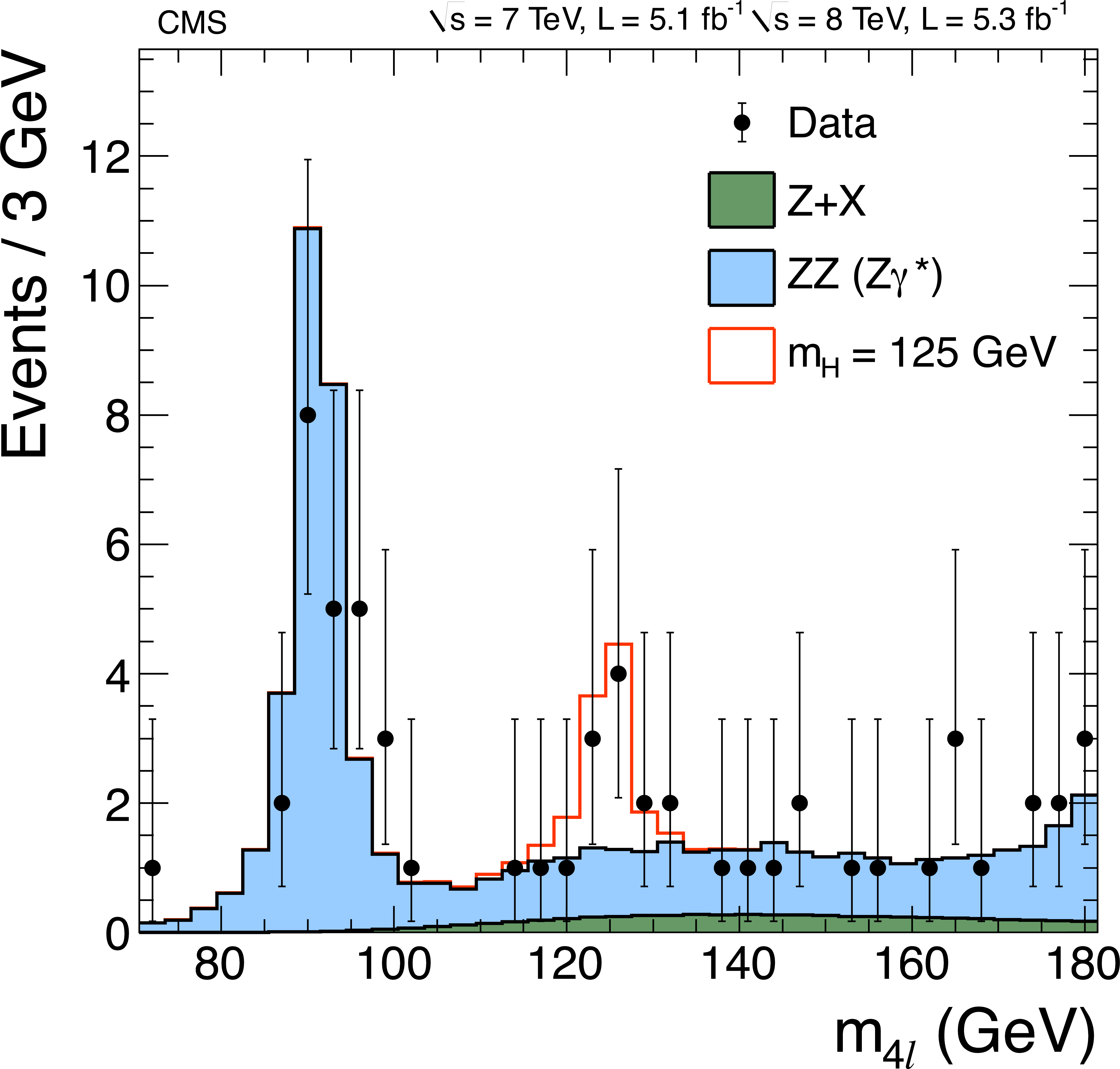
Figure 18:
Distribution of the observed four-lepton invariant mass from the combined 7 and 8 TeV data for the $ {\mathrm {H}} \to {\mathrm {Z}} {\mathrm {Z}}\to 4\ell $ analysis (points). The prediction for the expected $ {\mathrm {Z}}$+X and $ {\mathrm {Z}} {\mathrm {Z}}( {\mathrm {Z}}\gamma ^*)$ background are shown by the dark and light histogram, respectively. The open histogram gives the expected distribution for a Higgs boson of mass 125 GeV . |

png pdf |
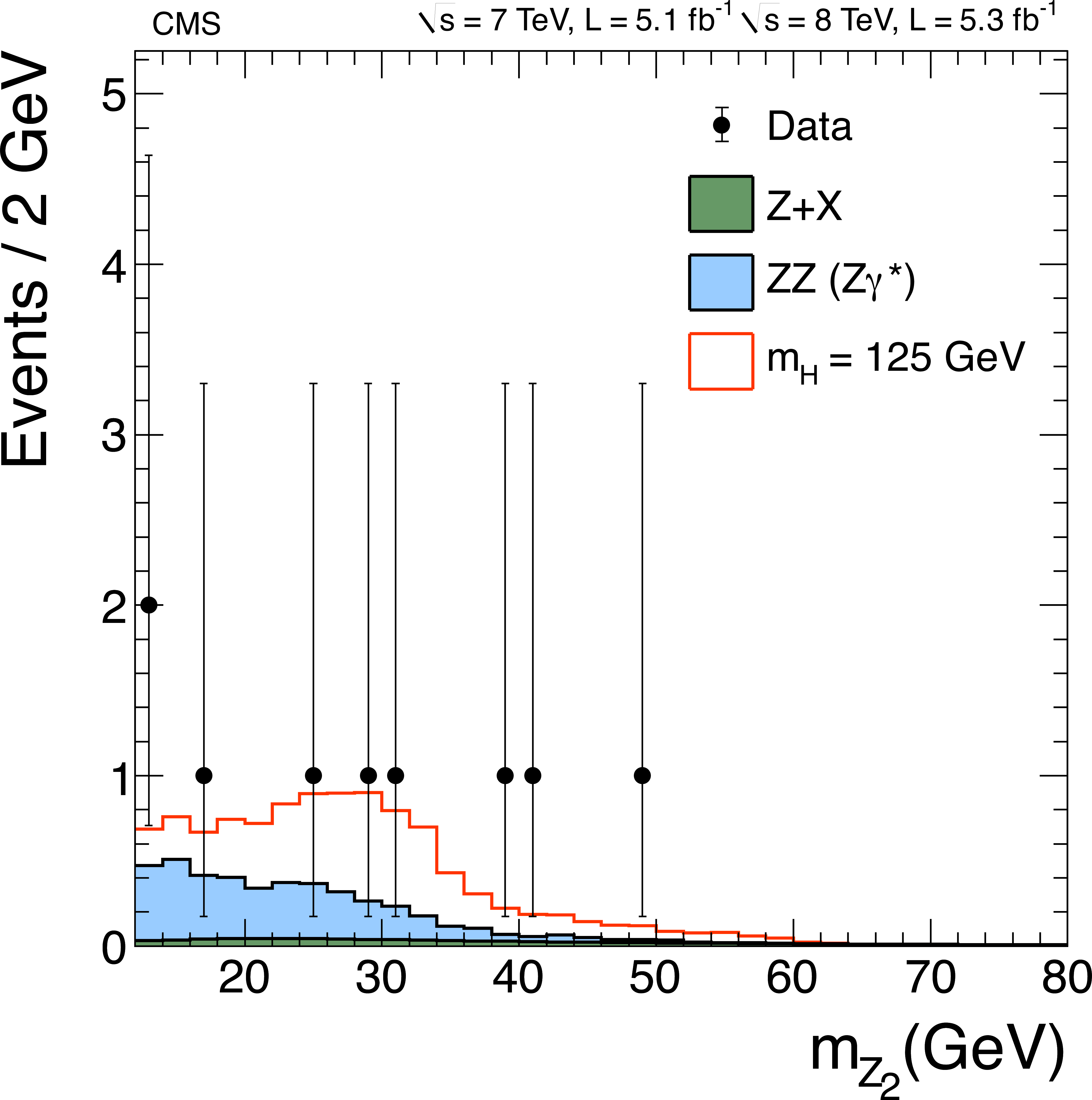
Figure 19-a:
Distributions of the observed $ {\mathrm {Z}}_1$ (left) and $ {\mathrm {Z}}_2$ (right) dilepton invariant masses for four-lepton events in the mass range 121.5 $< m_{4\ell } < $130.5 GeV for the combined 7 and 8 TeV data (points) . The shaded histograms show the predictions for the background distributions, and the open histogram for a Higgs boson with a mass of 125 GeV . |
png pdf |
Figure 19-b:
Distributions of the observed $ {\mathrm {Z}}_1$ (left) and $ {\mathrm {Z}}_2$ (right) dilepton invariant masses for four-lepton events in the mass range 121.5 $< m_{4\ell } < $130.5 GeV for the combined 7 and 8 TeV data (points) . The shaded histograms show the predictions for the background distributions, and the open histogram for a Higgs boson with a mass of 125 GeV . |
png pdf |
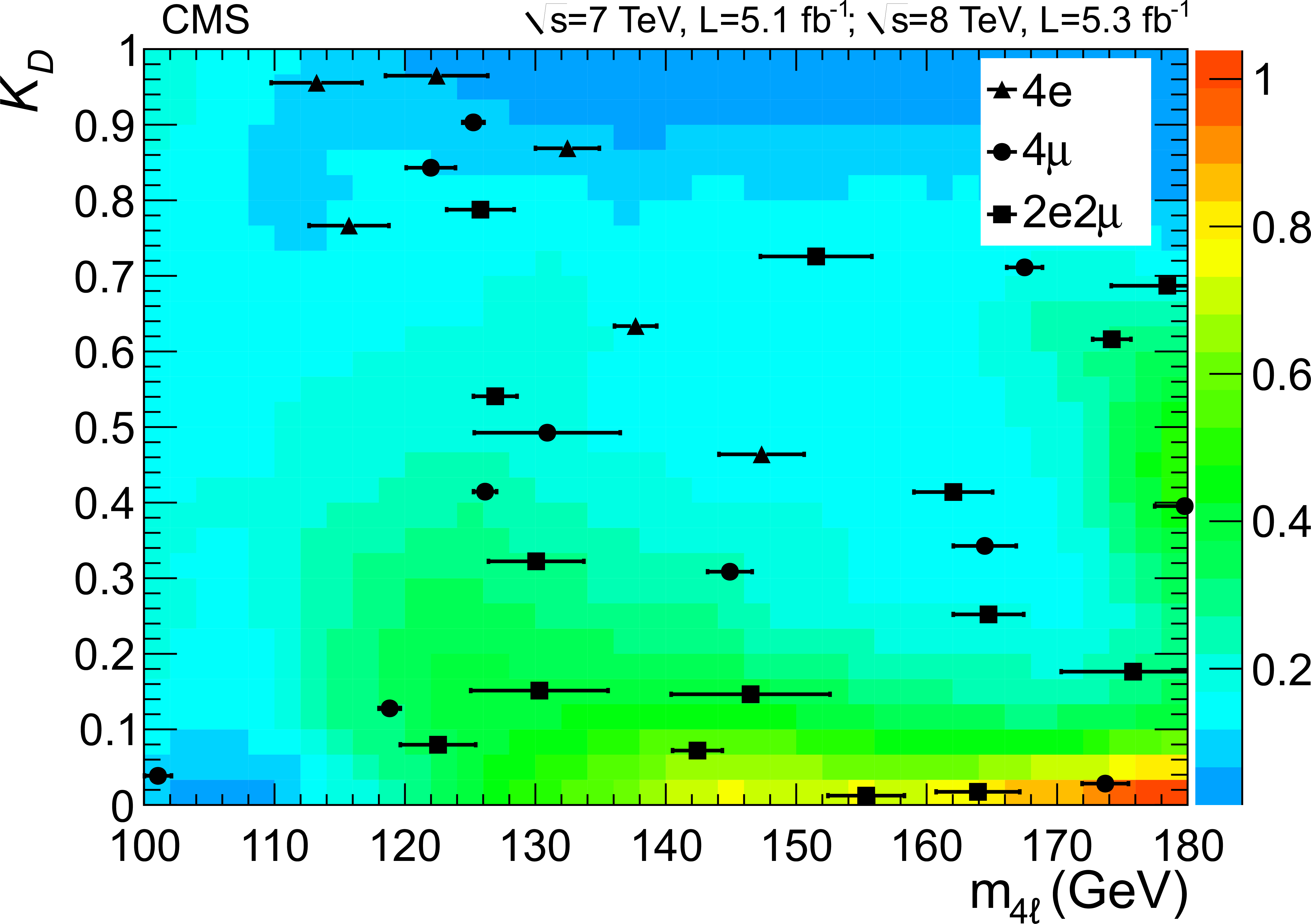
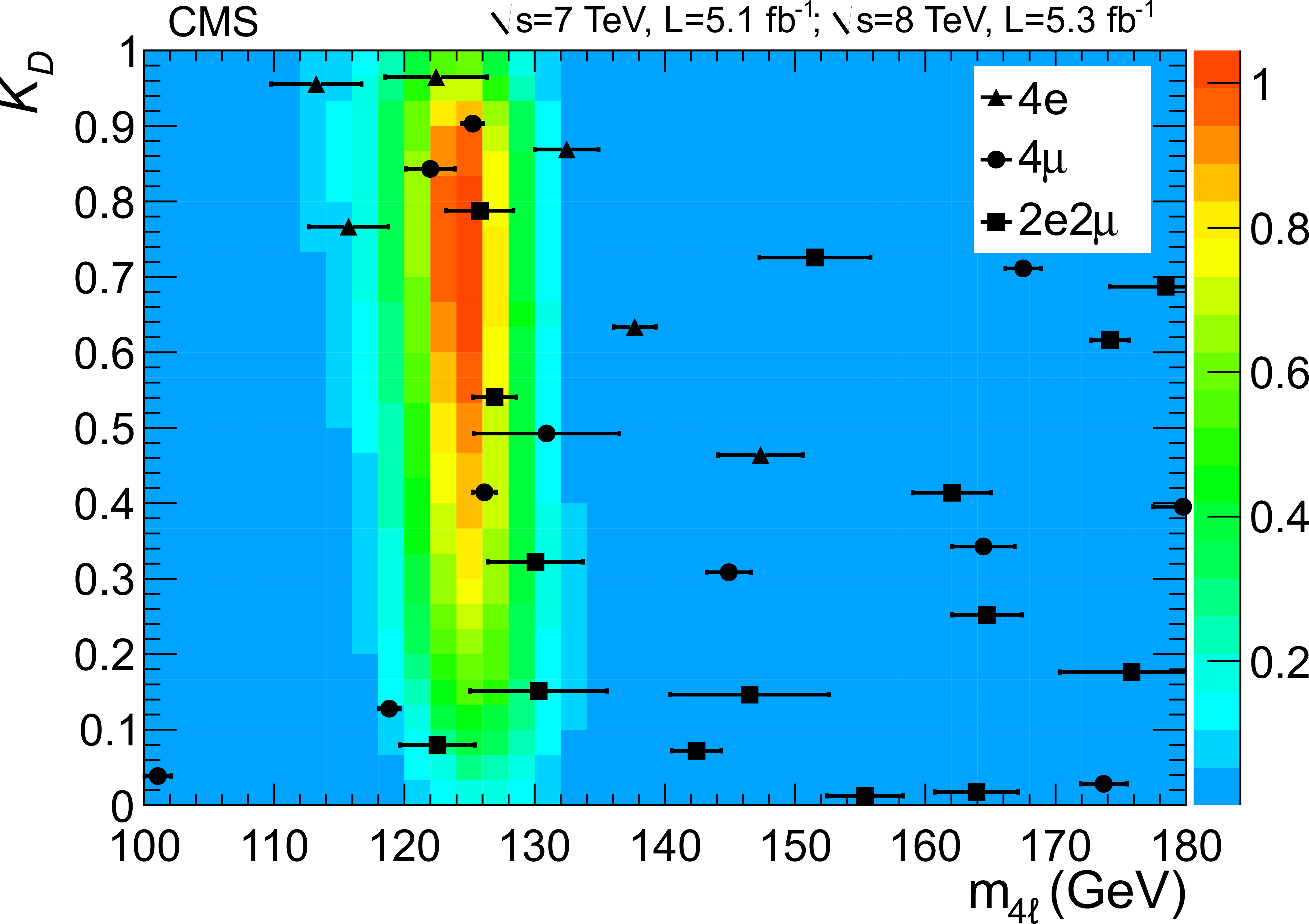
Figure 20-a:
The two-dimensional distribution of the kinematic discriminant $K_{D}$ versus $m_{4\ell }$ for selected $4\ell $ events in the combined 7 and 8 TeV data. Events in the three different final states are designated by symbols shown in the legend. The horizontal error bars indicate the estimated per-event mass resolution deduced from the combination of the per-lepton momentum uncertainties. The contours in the upper plot show the event density for the background expectation, and in the lower plot the contours for a SM Higgs boson with $ {m_{ {\mathrm {H}} }}$ = 125 GeV (both in arbitrary units). |
png pdf |
Figure 20-b:
The two-dimensional distribution of the kinematic discriminant $K_{D}$ versus $m_{4\ell }$ for selected $4\ell $ events in the combined 7 and 8 TeV data. Events in the three different final states are designated by symbols shown in the legend. The horizontal error bars indicate the estimated per-event mass resolution deduced from the combination of the per-lepton momentum uncertainties. The contours in the upper plot show the event density for the background expectation, and in the lower plot the contours for a SM Higgs boson with $ {m_{ {\mathrm {H}} }}$ = 125 GeV (both in arbitrary units). |
png pdf |
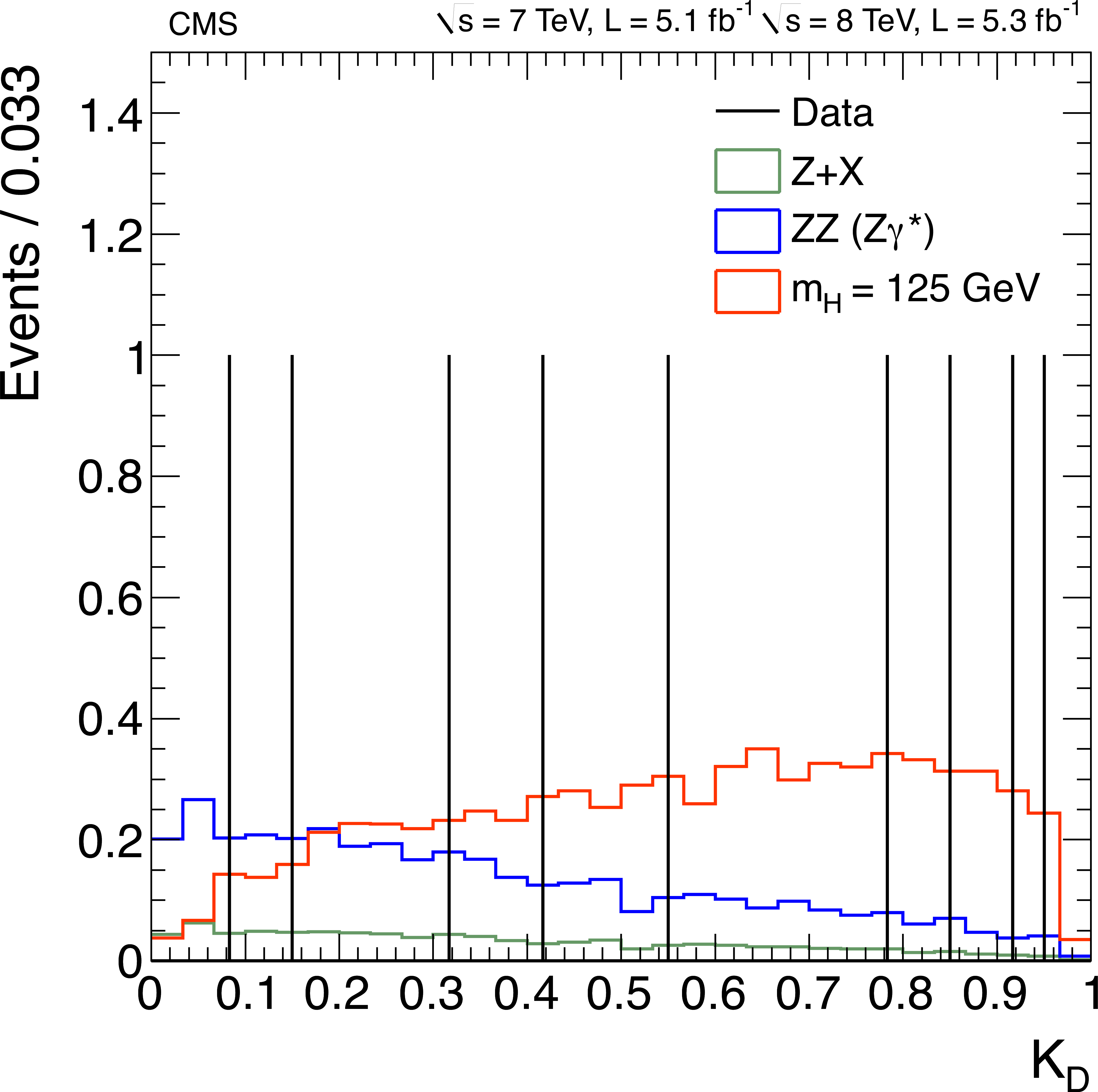
Figure 21-a:
Left: Distribution of the kinematic discriminant $K_D$ for $ {\mathrm {H}} \to {\mathrm {Z}} {\mathrm {Z}}\to 4\ell $ candidate events from the combined 7 and 8 TeV data (vertical lines) in the signal mass region $121.5 < m_{4\ell } < 130.5$ GeV . The predicted distributions for the Z+X and $ {\mathrm {Z}} {\mathrm {Z}}( {\mathrm {Z}}\gamma ^*)$ backgrounds and for a Higgs boson with a mass of 125 GeV are shown by the histograms. Right: The $m_{4\ell }$ distribution for data events with $K_D >$ 0.5 (points) and the predicted distributions for the backgrounds and a Higgs boson with a mass of 125 GeV (histograms). |
png pdf |
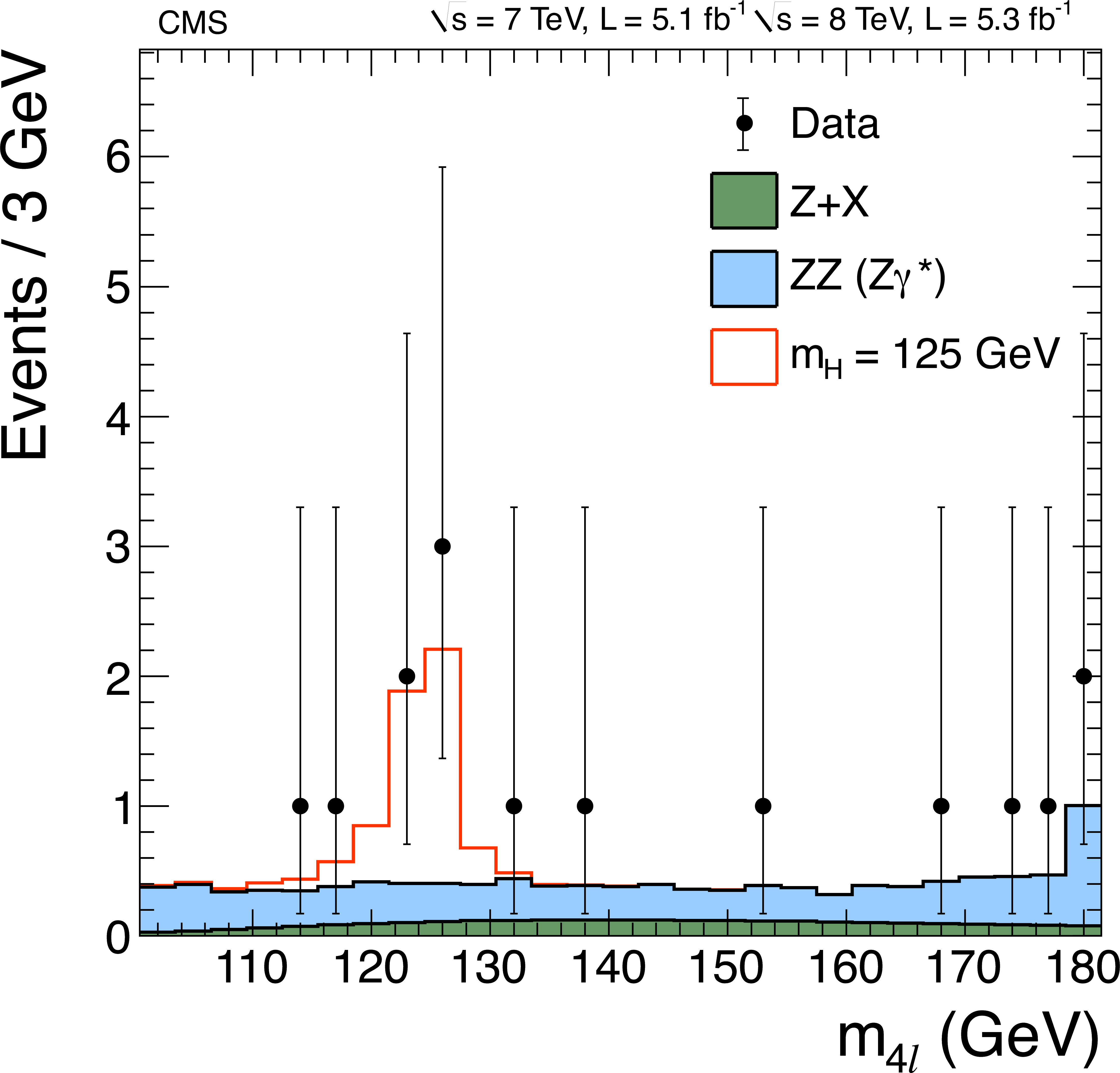
Figure 21-b:
Left: Distribution of the kinematic discriminant $K_D$ for $ {\mathrm {H}} \to {\mathrm {Z}} {\mathrm {Z}}\to 4\ell $ candidate events from the combined 7 and 8 TeV data (vertical lines) in the signal mass region $121.5 < m_{4\ell } < 130.5$ GeV . The predicted distributions for the Z+X and $ {\mathrm {Z}} {\mathrm {Z}}( {\mathrm {Z}}\gamma ^*)$ backgrounds and for a Higgs boson with a mass of 125 GeV are shown by the histograms. Right: The $m_{4\ell }$ distribution for data events with $K_D >$ 0.5 (points) and the predicted distributions for the backgrounds and a Higgs boson with a mass of 125 GeV (histograms). |

png pdf |
Figure 22-a:
Distributions of the azimuthal angle difference $ {\Delta \phi _{ {\ell } {\ell }}}$ between selected leptons in the 0-jet (left) and 1-jet (right) categories, for data (points), the main backgrounds (solid histograms), and a SM Higgs boson signal with $ {m_{ {\mathrm {H}} }}= $ 125 GeV (hatched histogram) at 8 TeV. The standard $ {\mathrm {W}} {\mathrm {W}}$ selection is applied. |

png pdf |
Figure 22-b:
Distributions of the azimuthal angle difference $ {\Delta \phi _{ {\ell } {\ell }}}$ between selected leptons in the 0-jet (left) and 1-jet (right) categories, for data (points), the main backgrounds (solid histograms), and a SM Higgs boson signal with $ {m_{ {\mathrm {H}} }}= $ 125 GeV (hatched histogram) at 8 TeV. The standard $ {\mathrm {W}} {\mathrm {W}}$ selection is applied. |

png pdf |
Figure 23-a:
Distributions of the dilepton invariant mass $ {m_{ {\ell } {\ell }}}$ of selected dileptons in the 0-jet (left) and 1-jet (right) categories, for data (points), the main backgrounds (solid histograms), and a SM Higgs boson with $ {m_{ {\mathrm {H}} }}=$ 125 GeV (hatched histogram) at 8 TeV. The standard $ {\mathrm {W}} {\mathrm {W}}$ selection is applied. The last bin contains overflows. |
png pdf |
Figure 23-b:
Distributions of the dilepton invariant mass $ {m_{ {\ell } {\ell }}}$ of selected dileptons in the 0-jet (left) and 1-jet (right) categories, for data (points), the main backgrounds (solid histograms), and a SM Higgs boson with $ {m_{ {\mathrm {H}} }}=$ 125 GeV (hatched histogram) at 8 TeV. The standard $ {\mathrm {W}} {\mathrm {W}}$ selection is applied. The last bin contains overflows. |
png pdf |
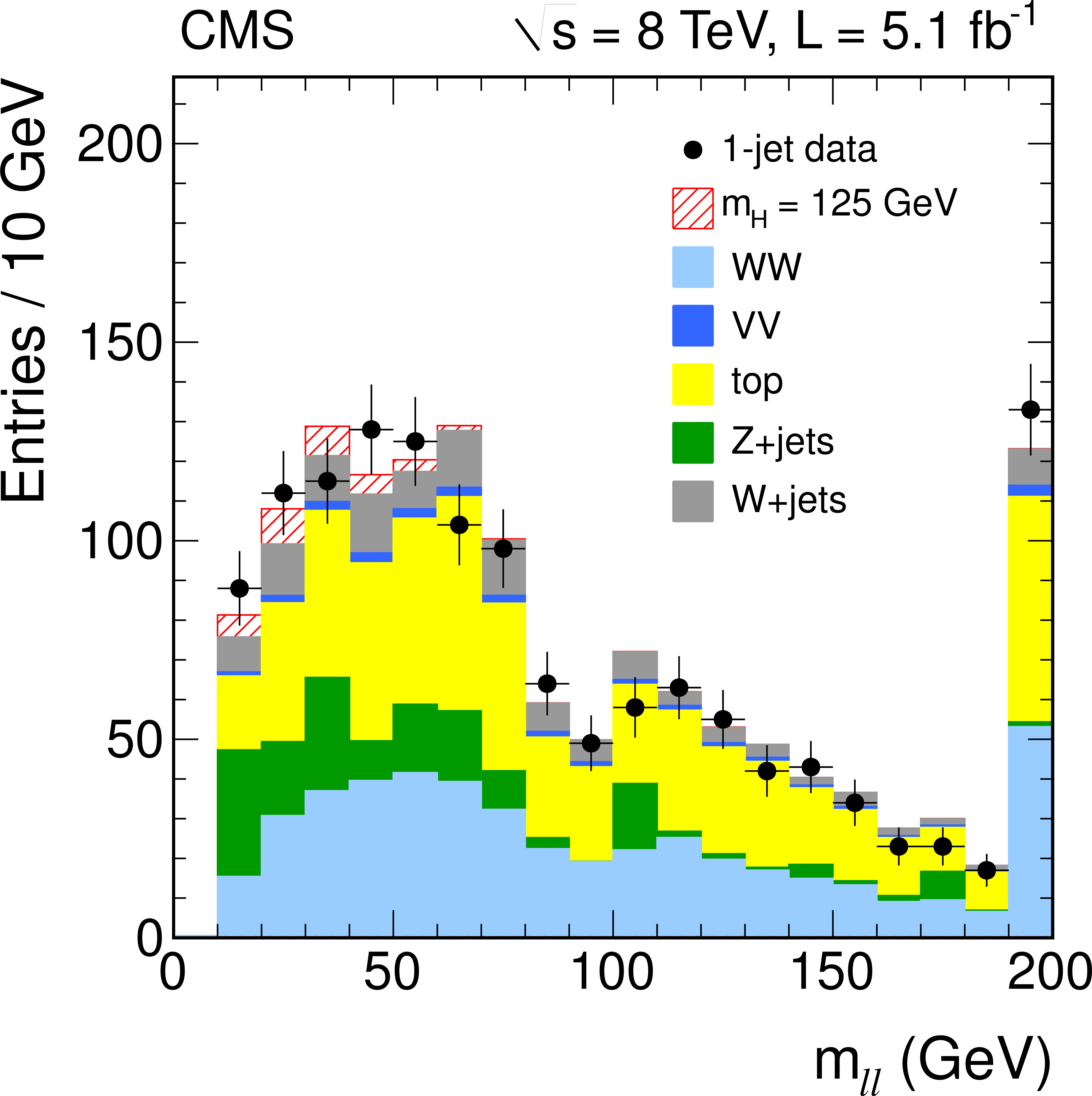
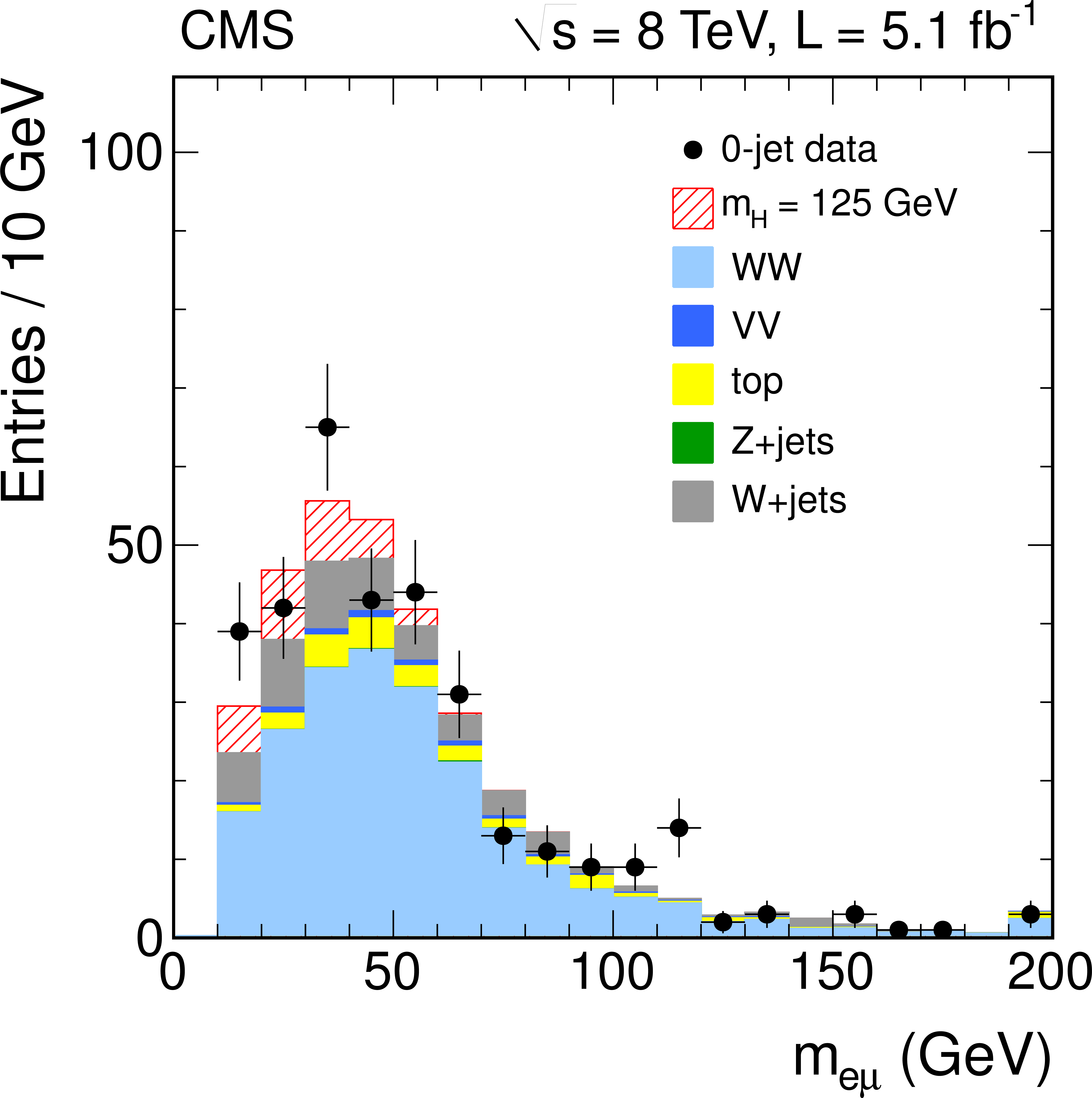
Figure 24-a:
Dilepton invariant mass distribution from the 0-jet (left) and 1-jet (right) $ {\mathrm {e}}\mu $ events from the 8 TeV data (points with error bars), and the prediction for the various backgrounds (solid histograms), and for a SM Higgs boson with $ {m_{ {\mathrm {H}} }}=$ 125 GeV (hatched histogram) at 8 TeV. The cut-based $ {\mathrm {H}} \to {\mathrm {W}} {\mathrm {W}}$ selection, except for the requirement on the dilepton mass itself, is applied. |
png pdf |
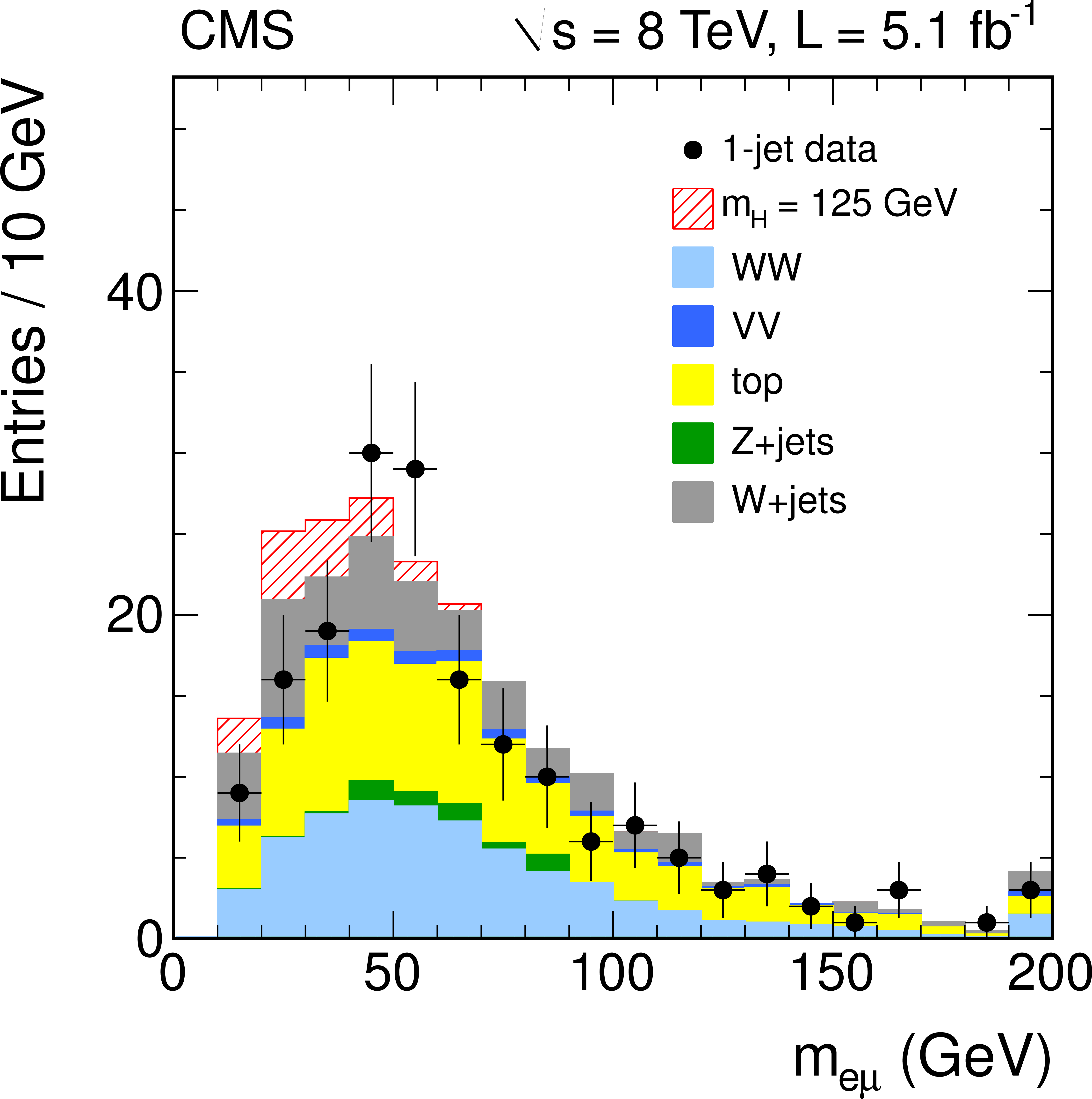
Figure 24-b:
Dilepton invariant mass distribution from the 0-jet (left) and 1-jet (right) $ {\mathrm {e}}\mu $ events from the 8 TeV data (points with error bars), and the prediction for the various backgrounds (solid histograms), and for a SM Higgs boson with $ {m_{ {\mathrm {H}} }}=$ 125 GeV (hatched histogram) at 8 TeV. The cut-based $ {\mathrm {H}} \to {\mathrm {W}} {\mathrm {W}}$ selection, except for the requirement on the dilepton mass itself, is applied. |
png pdf |
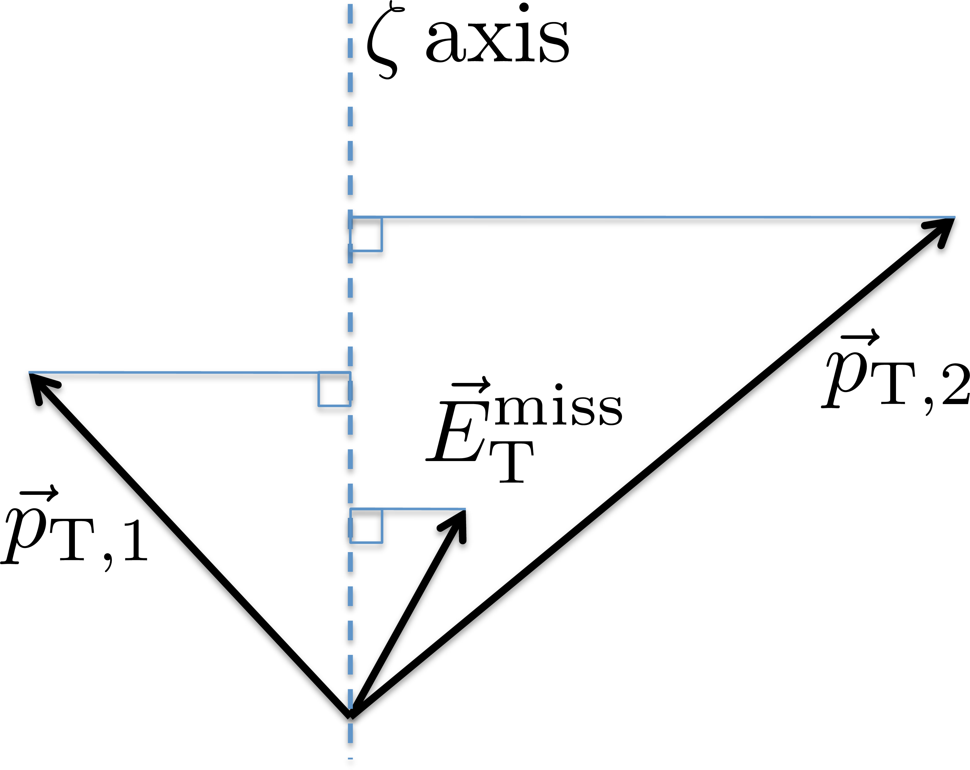
Figure 25:
The $\zeta $ axis and the projections onto this axis of $ \mathrm{E}_{\mathrm {T}}^{\text {miss}} $ and transverse momenta $\mathrm{p}_\mathrm {T,1}$ and $\mathrm{p}_\mathrm {T,2}$ of the two leptons. |
png pdf |
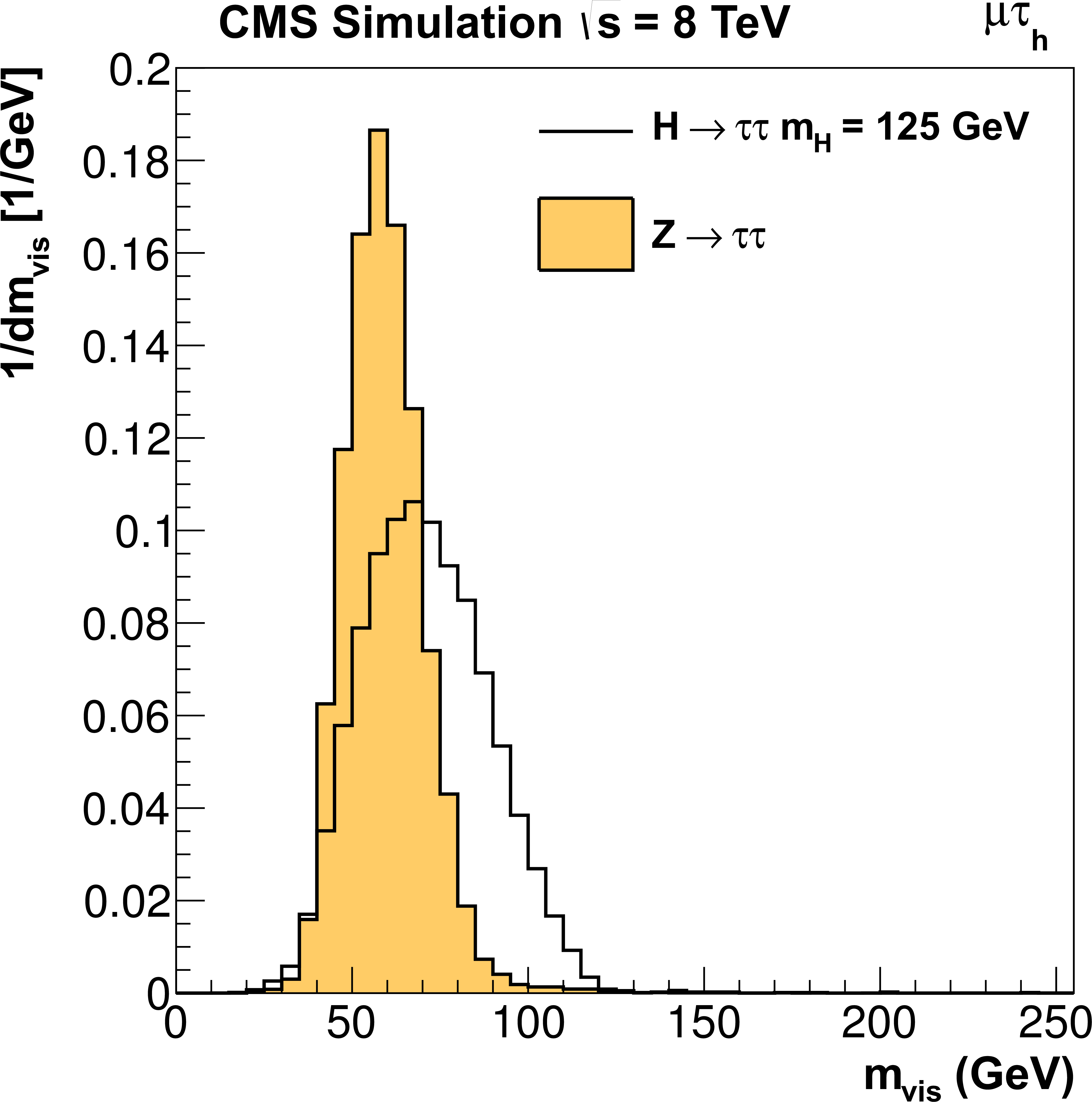
Figure 26-a:
Normalized distribution of the visible invariant mass $m_\text {vis}$ (left) and SVFit mass $m_{\tau \tau }$ (right) obtained from MC simulation in the $ {{\mu }} {\tau }_h$ channel for the $ {\mathrm {Z}}\to \tau \tau $ background (solid histogram) and a SM Higgs boson signal of mass $m_H=125 GeV $ (open histogram). |

png pdf |
Figure 26-b:
Normalized distribution of the visible invariant mass $m_\text {vis}$ (left) and SVFit mass $m_{\tau \tau }$ (right) obtained from MC simulation in the $ {{\mu }} {\tau }_h$ channel for the $ {\mathrm {Z}}\to \tau \tau $ background (solid histogram) and a SM Higgs boson signal of mass $m_H=125 GeV $ (open histogram). |
png pdf |
Figure 27-a:
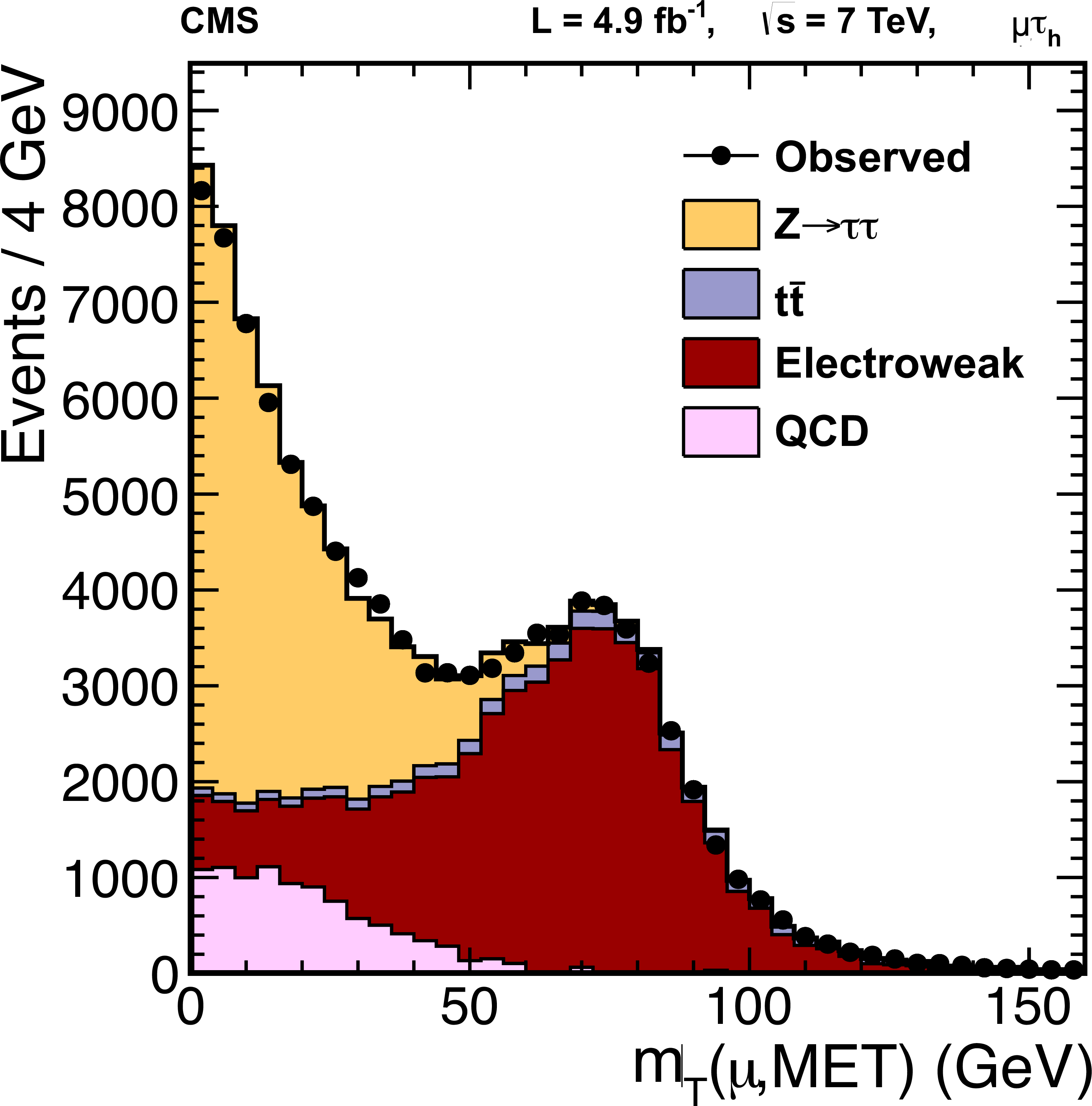
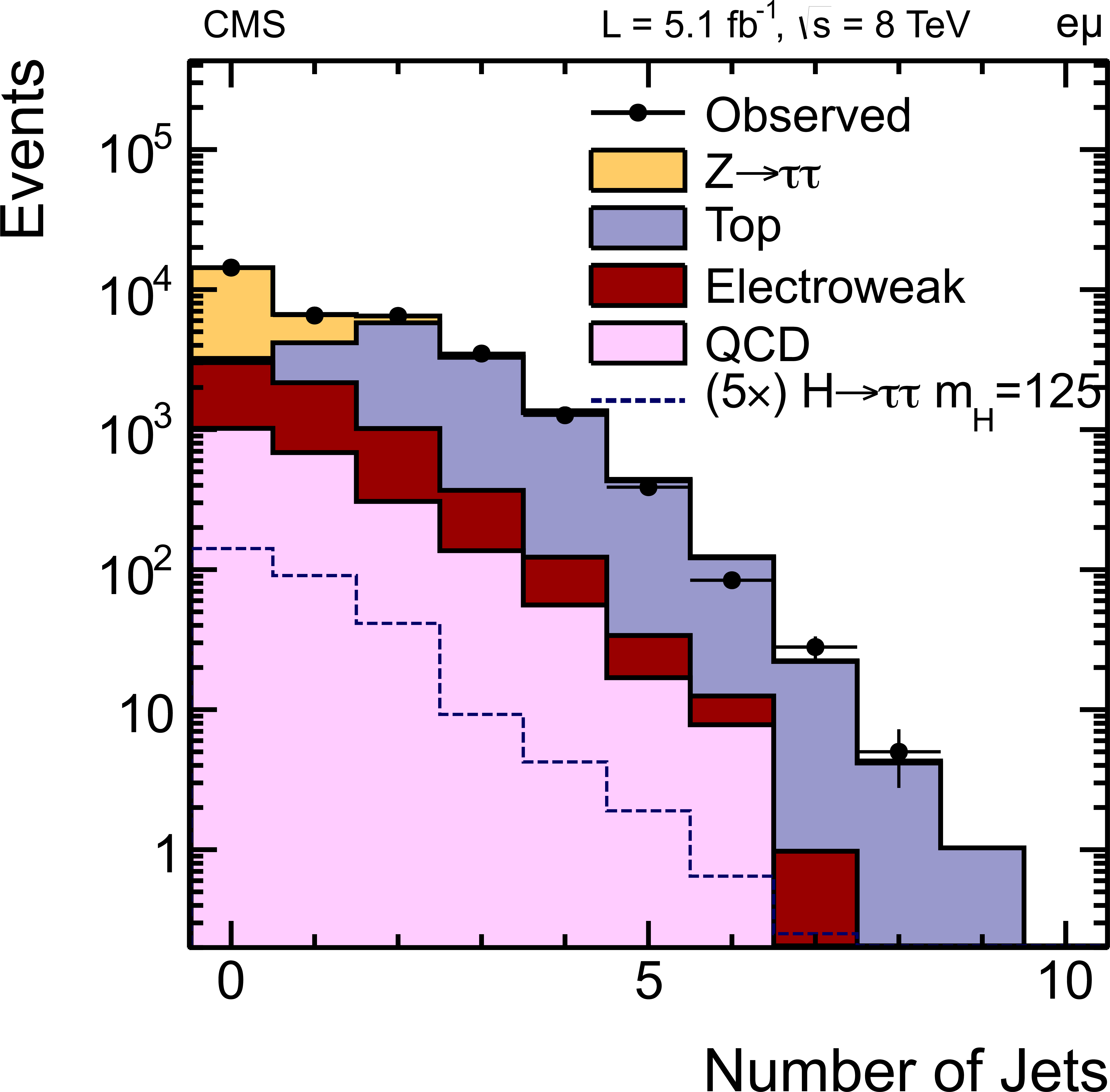
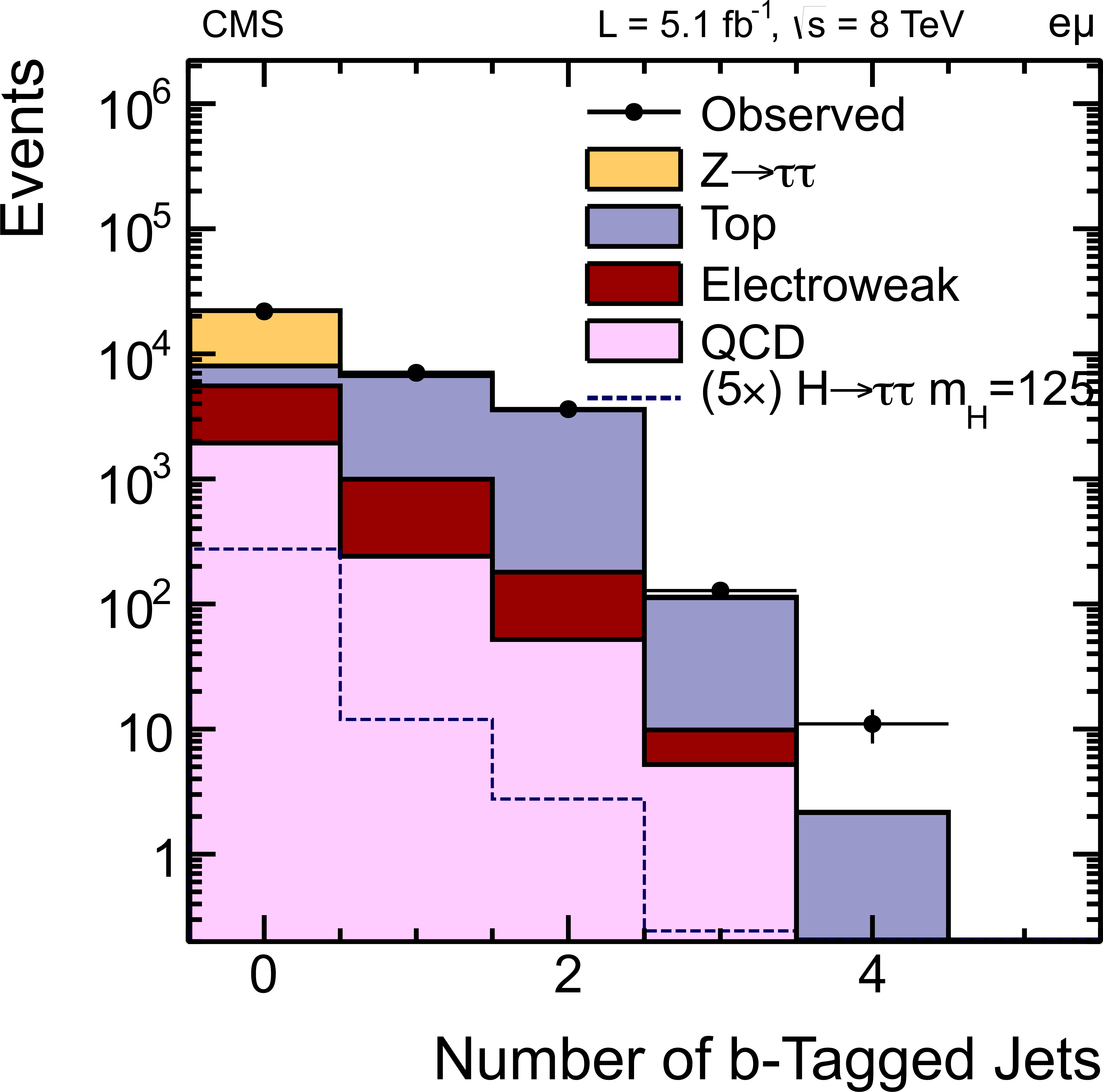
The observed distributions (points with error bars) for the (upper left) transverse mass $m_\mathrm {T}$ in the $ {{\mu }} {\tau }_h$ channel at $\sqrt {s}=$ 7 TeV; (upper right) $p_\zeta - 0.85 \cdot p_\zeta ^{\mathrm {vis}}$, (lower left) number of jets, and (lower right) number of b-tagged jets in the $ {\mathrm {e}} {{\mu }}$ channel at $\sqrt {s}=$ 8 TeV. The expected distributions from the various background sources are shown by the shaded histograms. In particular, the Electroweak background combines the expected contributions from W+jets, Z+jets, and diboson processes. The predictions for a SM Higgs boson with $ {m_{ {\mathrm {H}} }}=$ 125 GeV are given by the dotted histograms, multiplied by a factor of 5 for clarity. |
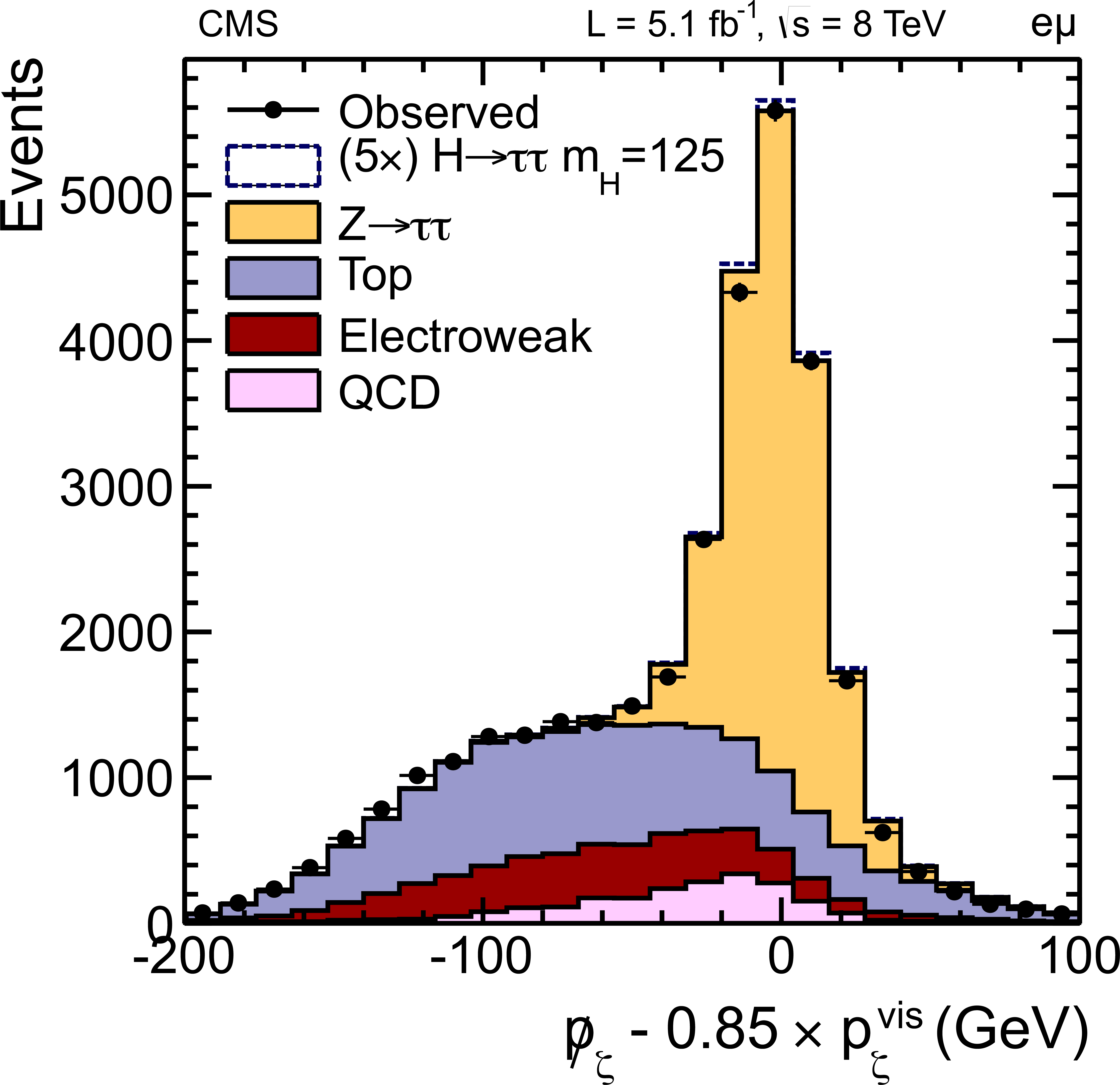
png pdf |
Figure 27-b:
The observed distributions (points with error bars) for the (upper left) transverse mass $m_\mathrm {T}$ in the $ {{\mu }} {\tau }_h$ channel at $\sqrt {s}=$ 7 TeV; (upper right) $p_\zeta - 0.85 \cdot p_\zeta ^{\mathrm {vis}}$, (lower left) number of jets, and (lower right) number of b-tagged jets in the $ {\mathrm {e}} {{\mu }}$ channel at $\sqrt {s}=$ 8 TeV. The expected distributions from the various background sources are shown by the shaded histograms. In particular, the Electroweak background combines the expected contributions from W+jets, Z+jets, and diboson processes. The predictions for a SM Higgs boson with $ {m_{ {\mathrm {H}} }}=$ 125 GeV are given by the dotted histograms, multiplied by a factor of 5 for clarity. |
png pdf |
Figure 27-c:
The observed distributions (points with error bars) for the (upper left) transverse mass $m_\mathrm {T}$ in the $ {{\mu }} {\tau }_h$ channel at $\sqrt {s}=$ 7 TeV; (upper right) $p_\zeta - 0.85 \cdot p_\zeta ^{\mathrm {vis}}$, (lower left) number of jets, and (lower right) number of b-tagged jets in the $ {\mathrm {e}} {{\mu }}$ channel at $\sqrt {s}=$ 8 TeV. The expected distributions from the various background sources are shown by the shaded histograms. In particular, the Electroweak background combines the expected contributions from W+jets, Z+jets, and diboson processes. The predictions for a SM Higgs boson with $ {m_{ {\mathrm {H}} }}=$ 125 GeV are given by the dotted histograms, multiplied by a factor of 5 for clarity. |
png pdf |
Figure 27-d:
The observed distributions (points with error bars) for the (upper left) transverse mass $m_\mathrm {T}$ in the $ {{\mu }} {\tau }_h$ channel at $\sqrt {s}=$ 7 TeV; (upper right) $p_\zeta - 0.85 \cdot p_\zeta ^{\mathrm {vis}}$, (lower left) number of jets, and (lower right) number of b-tagged jets in the $ {\mathrm {e}} {{\mu }}$ channel at $\sqrt {s}=$ 8 TeV. The expected distributions from the various background sources are shown by the shaded histograms. In particular, the Electroweak background combines the expected contributions from W+jets, Z+jets, and diboson processes. The predictions for a SM Higgs boson with $ {m_{ {\mathrm {H}} }}=$ 125 GeV are given by the dotted histograms, multiplied by a factor of 5 for clarity. |
png pdf |
Figure 28-a:
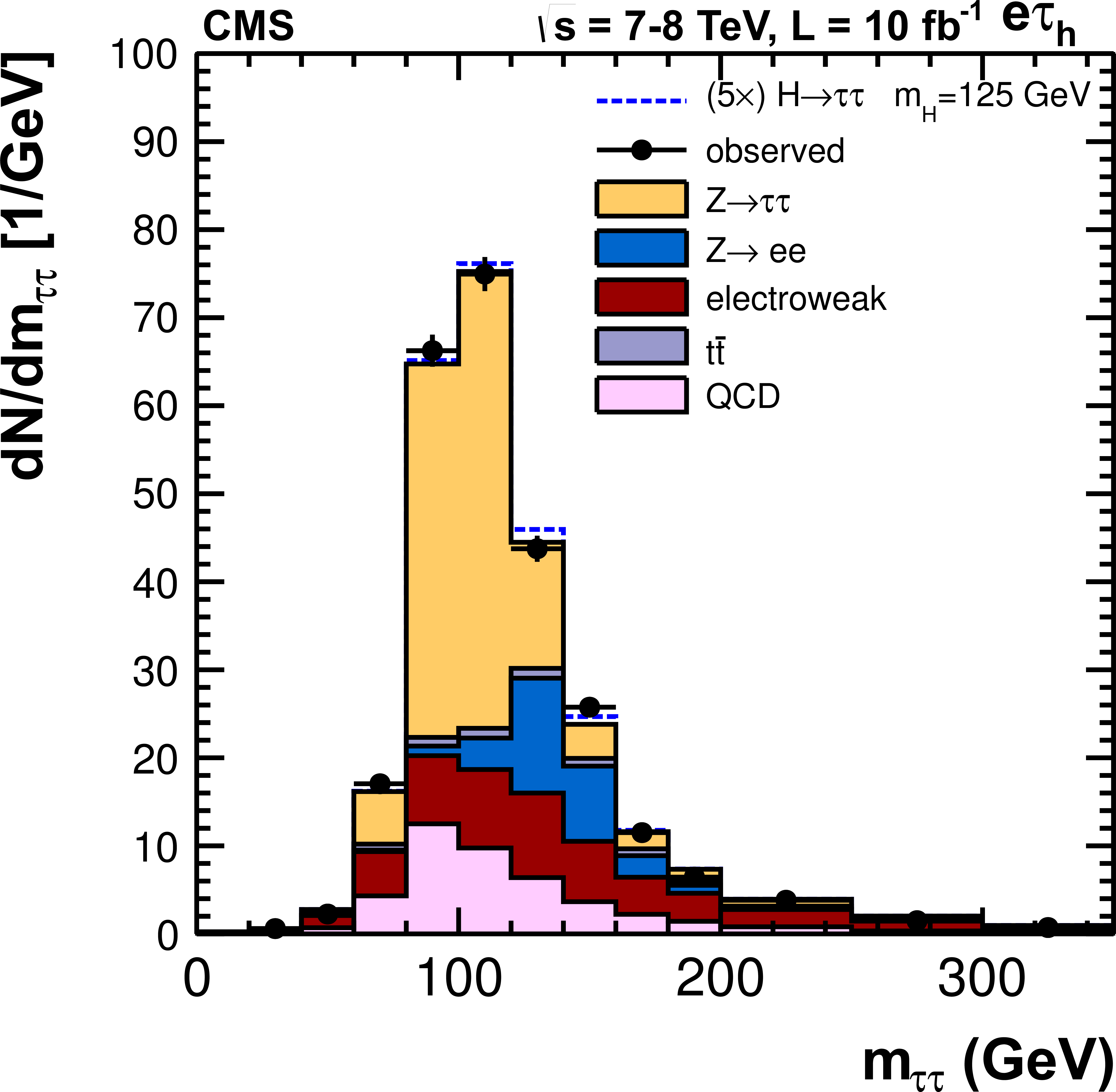
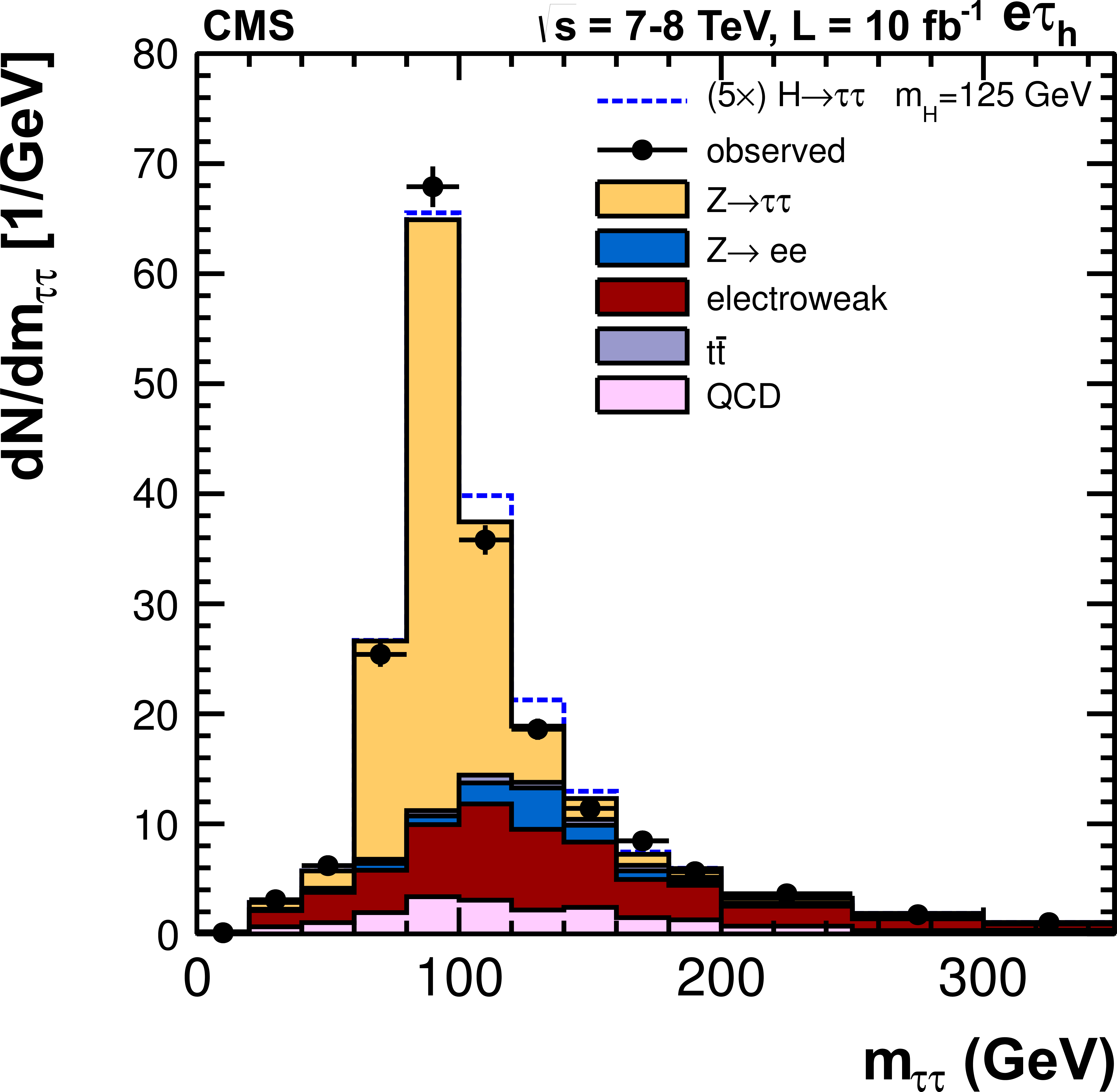
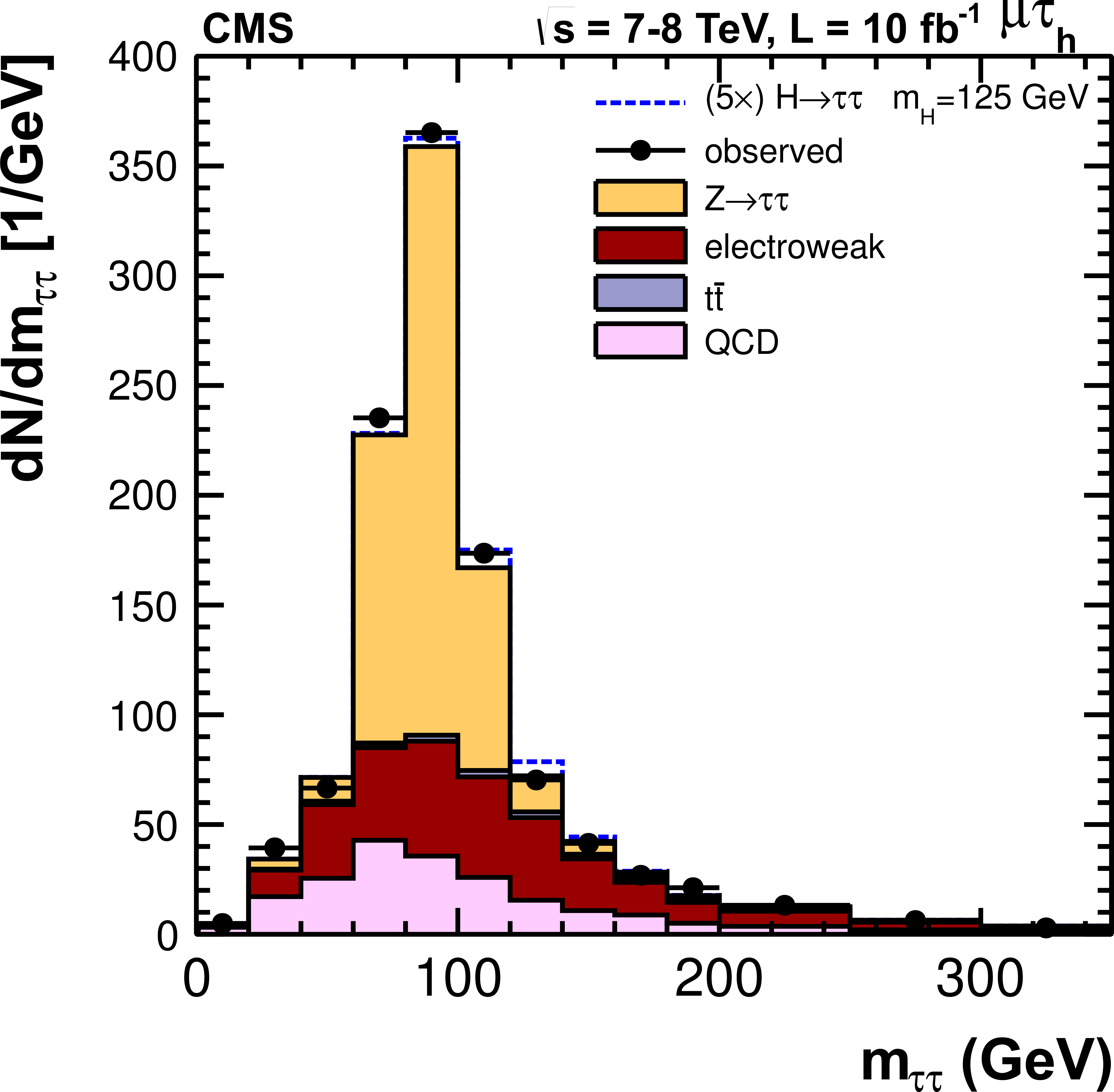
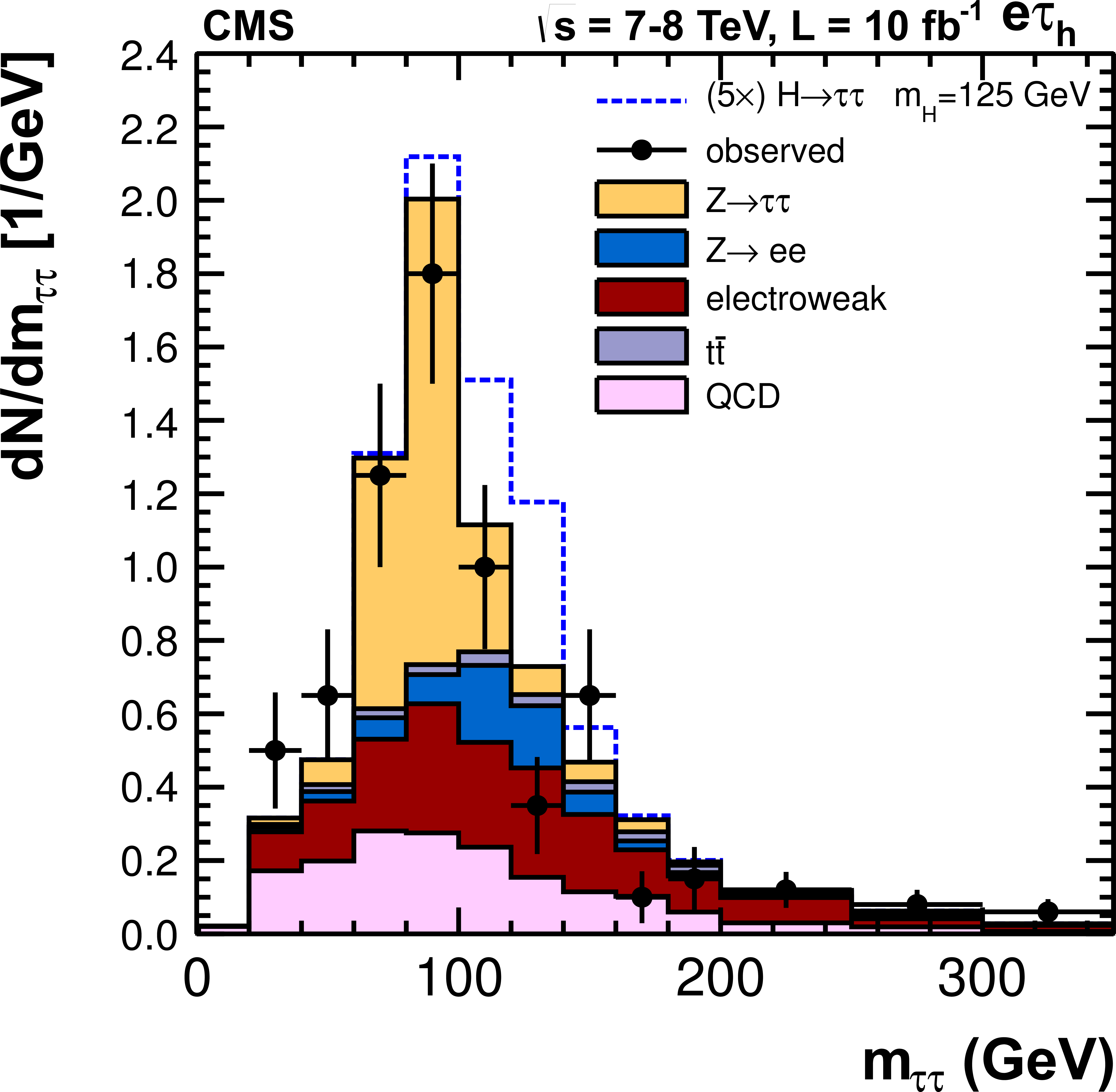
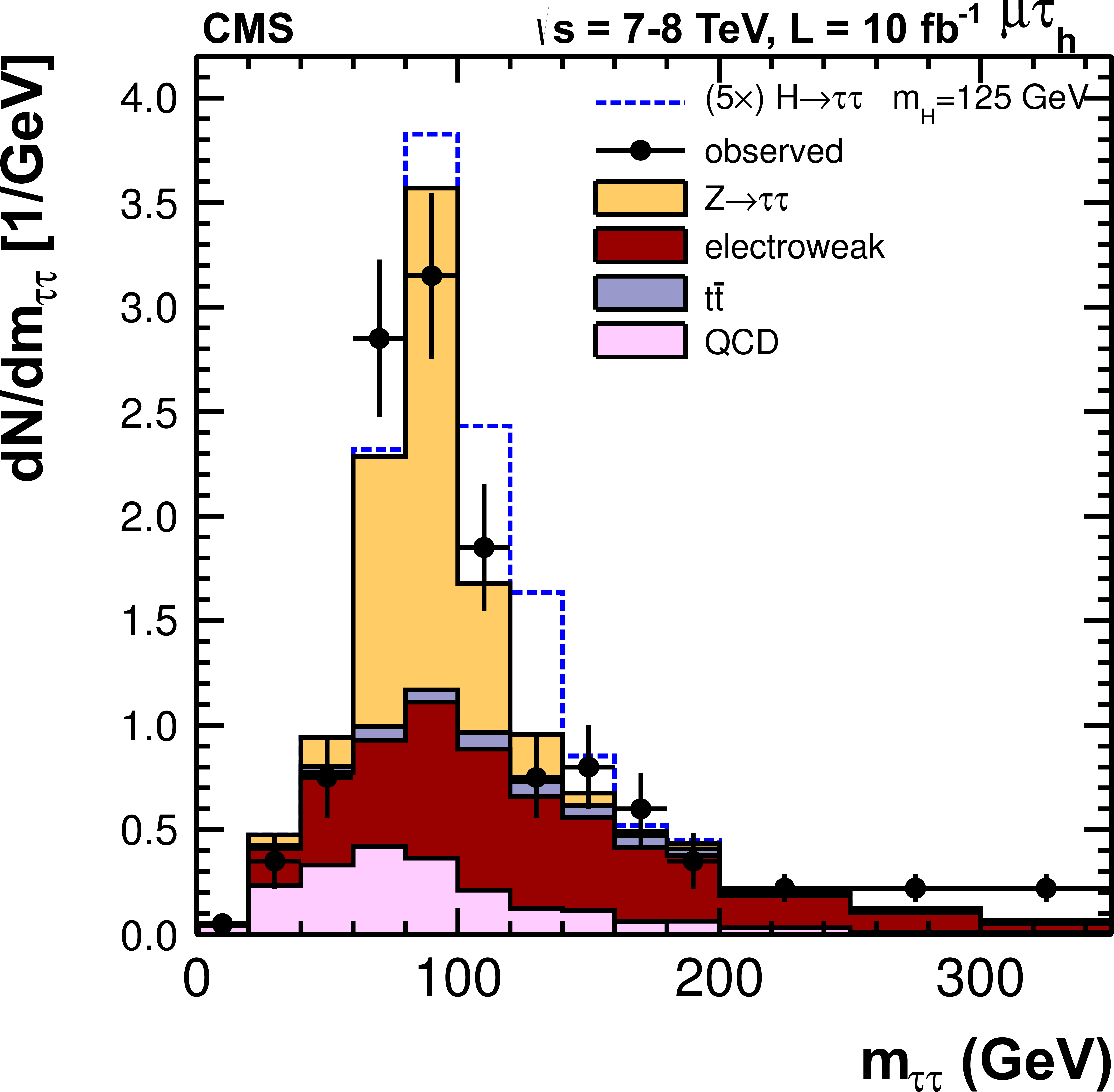
Observed (points with error bars) and expected (histograms) $m_{\tau \tau }$ distributions for the $ {\mathrm {e}} {\tau }_h$ (left) and $\mu {\tau }_h$ (right) channels, and, from top to bottom, the 0-jet, 1-jet, and VBF categories for the combined 7 and 8 TeV data sets. In the 0- and 1-jet categories, the low- and high-$ {p_{\mathrm {T}}} $ subcategories have been summed. The electroweak background combines the expected contributions from W+jets, Z+jets, and diboson processes. In the case of $ {\mathrm {e}} {\tau }_h$, the $ {\mathrm {Z}}\to {\mathrm {e}} {\mathrm {e}}$ background is shown separately. The dotted histogram shows the expected distribution for a SM Higgs boson with $ {m_{ {\mathrm {H}} }}=$ 125 GeV (multiplied by a factor of 5 for clarity). |
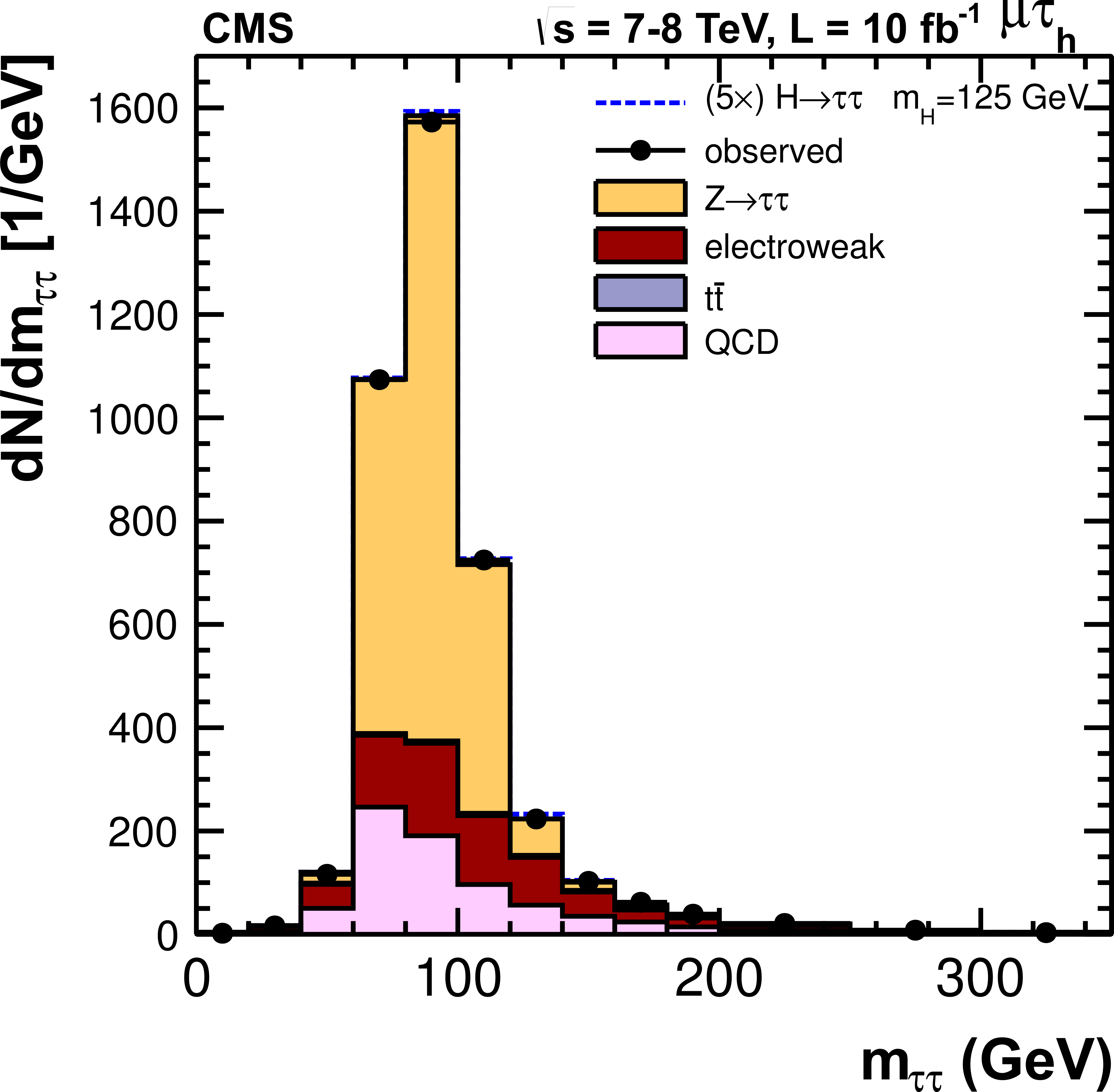
png pdf |
Figure 28-b:
Observed (points with error bars) and expected (histograms) $m_{\tau \tau }$ distributions for the $ {\mathrm {e}} {\tau }_h$ (left) and $\mu {\tau }_h$ (right) channels, and, from top to bottom, the 0-jet, 1-jet, and VBF categories for the combined 7 and 8 TeV data sets. In the 0- and 1-jet categories, the low- and high-$ {p_{\mathrm {T}}} $ subcategories have been summed. The electroweak background combines the expected contributions from W+jets, Z+jets, and diboson processes. In the case of $ {\mathrm {e}} {\tau }_h$, the $ {\mathrm {Z}}\to {\mathrm {e}} {\mathrm {e}}$ background is shown separately. The dotted histogram shows the expected distribution for a SM Higgs boson with $ {m_{ {\mathrm {H}} }}=$ 125 GeV (multiplied by a factor of 5 for clarity). |
png pdf |
Figure 28-c:
Observed (points with error bars) and expected (histograms) $m_{\tau \tau }$ distributions for the $ {\mathrm {e}} {\tau }_h$ (left) and $\mu {\tau }_h$ (right) channels, and, from top to bottom, the 0-jet, 1-jet, and VBF categories for the combined 7 and 8 TeV data sets. In the 0- and 1-jet categories, the low- and high-$ {p_{\mathrm {T}}} $ subcategories have been summed. The electroweak background combines the expected contributions from W+jets, Z+jets, and diboson processes. In the case of $ {\mathrm {e}} {\tau }_h$, the $ {\mathrm {Z}}\to {\mathrm {e}} {\mathrm {e}}$ background is shown separately. The dotted histogram shows the expected distribution for a SM Higgs boson with $ {m_{ {\mathrm {H}} }}=$ 125 GeV (multiplied by a factor of 5 for clarity). |
png pdf |
Figure 28-d:
Observed (points with error bars) and expected (histograms) $m_{\tau \tau }$ distributions for the $ {\mathrm {e}} {\tau }_h$ (left) and $\mu {\tau }_h$ (right) channels, and, from top to bottom, the 0-jet, 1-jet, and VBF categories for the combined 7 and 8 TeV data sets. In the 0- and 1-jet categories, the low- and high-$ {p_{\mathrm {T}}} $ subcategories have been summed. The electroweak background combines the expected contributions from W+jets, Z+jets, and diboson processes. In the case of $ {\mathrm {e}} {\tau }_h$, the $ {\mathrm {Z}}\to {\mathrm {e}} {\mathrm {e}}$ background is shown separately. The dotted histogram shows the expected distribution for a SM Higgs boson with $ {m_{ {\mathrm {H}} }}=$ 125 GeV (multiplied by a factor of 5 for clarity). |
png pdf |
Figure 28-e:
Observed (points with error bars) and expected (histograms) $m_{\tau \tau }$ distributions for the $ {\mathrm {e}} {\tau }_h$ (left) and $\mu {\tau }_h$ (right) channels, and, from top to bottom, the 0-jet, 1-jet, and VBF categories for the combined 7 and 8 TeV data sets. In the 0- and 1-jet categories, the low- and high-$ {p_{\mathrm {T}}} $ subcategories have been summed. The electroweak background combines the expected contributions from W+jets, Z+jets, and diboson processes. In the case of $ {\mathrm {e}} {\tau }_h$, the $ {\mathrm {Z}}\to {\mathrm {e}} {\mathrm {e}}$ background is shown separately. The dotted histogram shows the expected distribution for a SM Higgs boson with $ {m_{ {\mathrm {H}} }}=$ 125 GeV (multiplied by a factor of 5 for clarity). |
png pdf |
Figure 28-f:
Observed (points with error bars) and expected (histograms) $m_{\tau \tau }$ distributions for the $ {\mathrm {e}} {\tau }_h$ (left) and $\mu {\tau }_h$ (right) channels, and, from top to bottom, the 0-jet, 1-jet, and VBF categories for the combined 7 and 8 TeV data sets. In the 0- and 1-jet categories, the low- and high-$ {p_{\mathrm {T}}} $ subcategories have been summed. The electroweak background combines the expected contributions from W+jets, Z+jets, and diboson processes. In the case of $ {\mathrm {e}} {\tau }_h$, the $ {\mathrm {Z}}\to {\mathrm {e}} {\mathrm {e}}$ background is shown separately. The dotted histogram shows the expected distribution for a SM Higgs boson with $ {m_{ {\mathrm {H}} }}=$ 125 GeV (multiplied by a factor of 5 for clarity). |
png pdf |
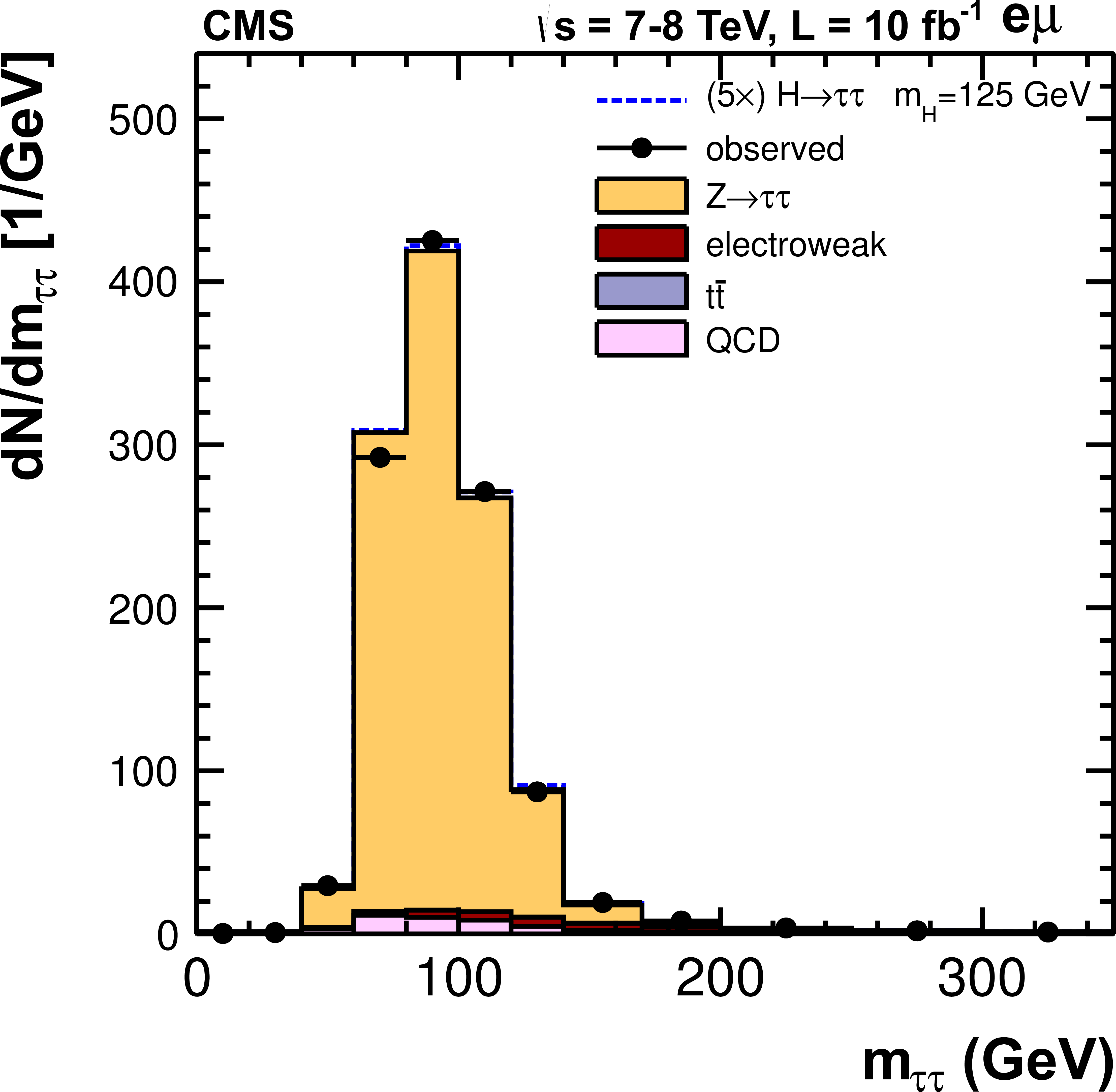
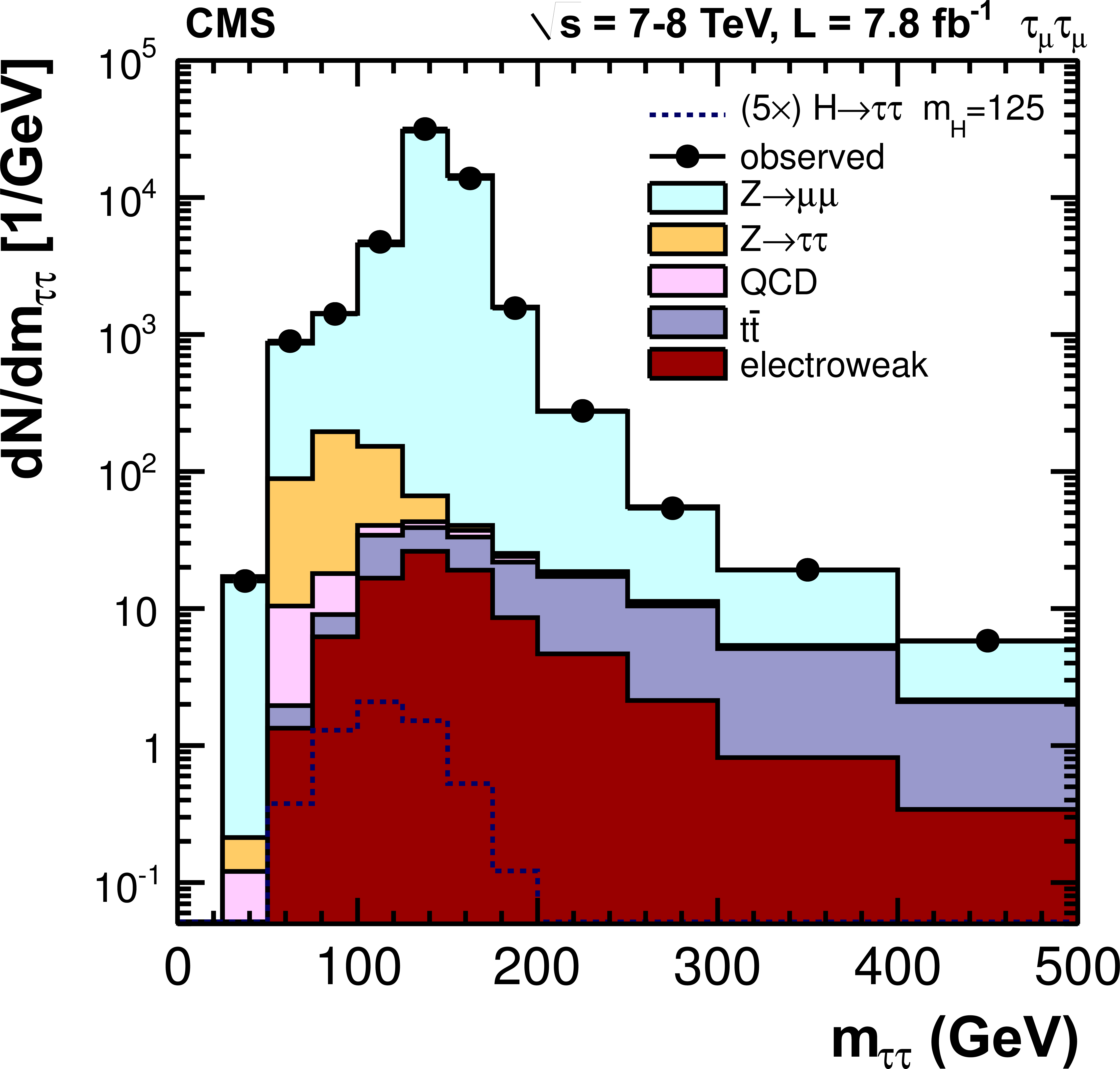
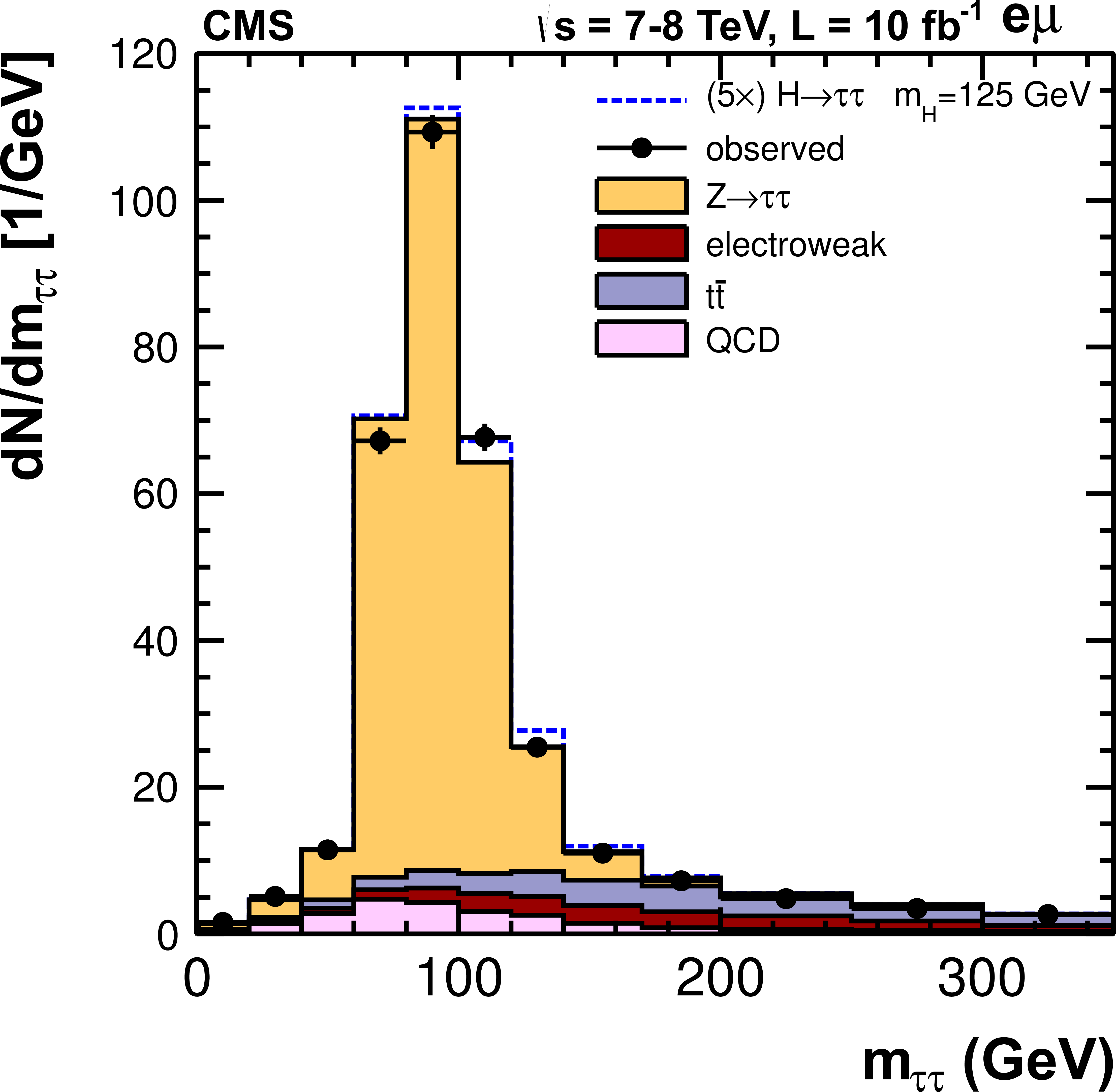
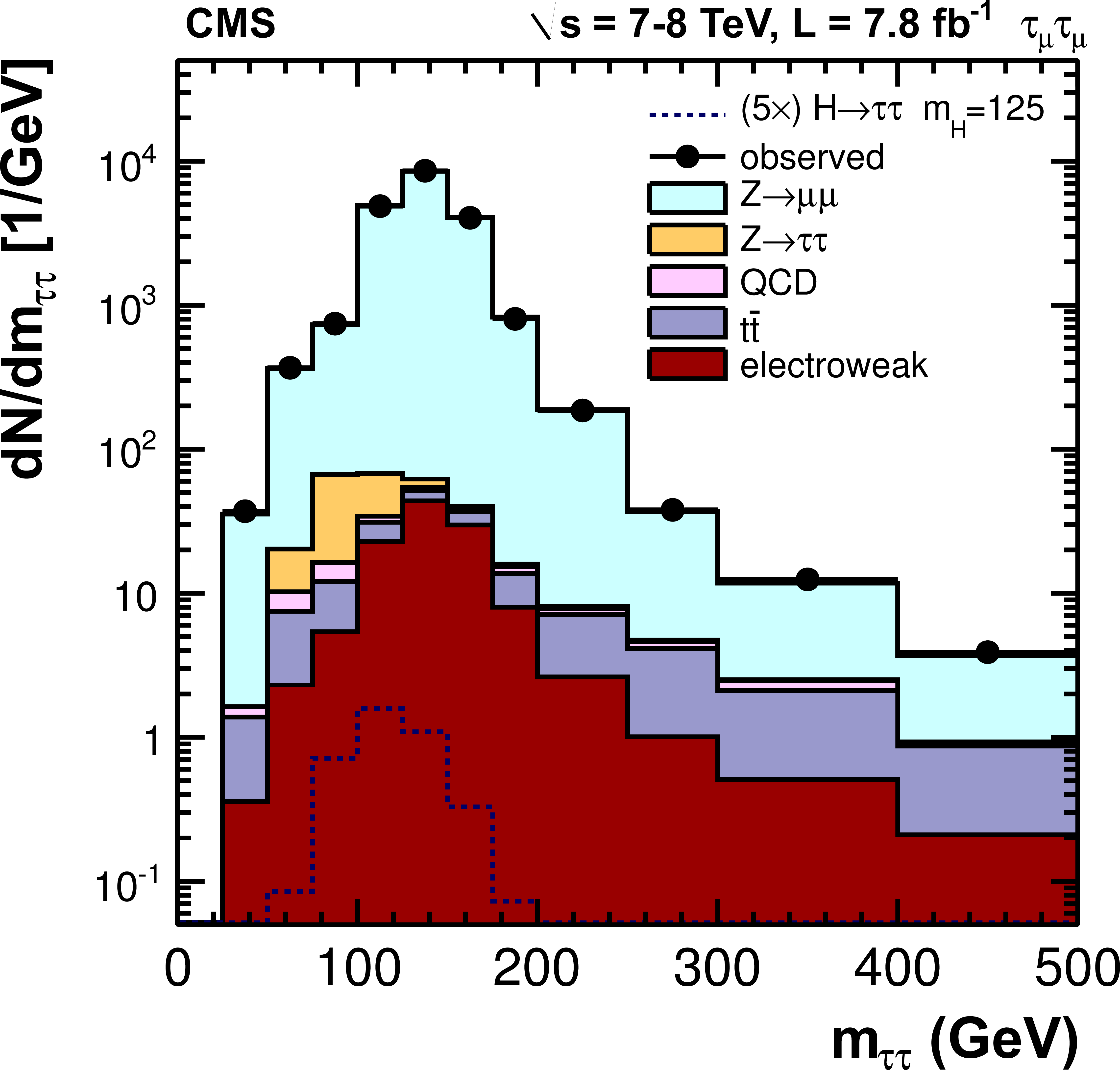
Figure 29-a:
Observed (points with error bars) and expected (histograms) $m_{\tau \tau }$ distributions for the $ {\mathrm {e}}\mu $ (left) and $\mu \mu $ (right) channels, and, from top to bottom, the 0-jet, 1-jet, and VBF categories for the combined 7 and 8 TeV data sets. In the 0- and 1-jet categories, the low- and high-$ {p_{\mathrm {T}}} $ subcategories have been summed. The electroweak background combines the contributions from $ {\mathrm {W}}$+jets, $ {\mathrm {Z}}$+jets, and diboson processes. In the case of $\mu \mu $, the $ {\mathrm {Z}}\to \mu \mu $ background is shown separately. The dotted histogram shows the expected distribution for a SM Higgs boson with $ {m_{ {\mathrm {H}} }}=$ 125 GeV (multiplied by a factor of 5 for clarity). |
png pdf |
Figure 29-b:
Observed (points with error bars) and expected (histograms) $m_{\tau \tau }$ distributions for the $ {\mathrm {e}}\mu $ (left) and $\mu \mu $ (right) channels, and, from top to bottom, the 0-jet, 1-jet, and VBF categories for the combined 7 and 8 TeV data sets. In the 0- and 1-jet categories, the low- and high-$ {p_{\mathrm {T}}} $ subcategories have been summed. The electroweak background combines the contributions from $ {\mathrm {W}}$+jets, $ {\mathrm {Z}}$+jets, and diboson processes. In the case of $\mu \mu $, the $ {\mathrm {Z}}\to \mu \mu $ background is shown separately. The dotted histogram shows the expected distribution for a SM Higgs boson with $ {m_{ {\mathrm {H}} }}=$ 125 GeV (multiplied by a factor of 5 for clarity). |
png pdf |
Figure 29-c:
Observed (points with error bars) and expected (histograms) $m_{\tau \tau }$ distributions for the $ {\mathrm {e}}\mu $ (left) and $\mu \mu $ (right) channels, and, from top to bottom, the 0-jet, 1-jet, and VBF categories for the combined 7 and 8 TeV data sets. In the 0- and 1-jet categories, the low- and high-$ {p_{\mathrm {T}}} $ subcategories have been summed. The electroweak background combines the contributions from $ {\mathrm {W}}$+jets, $ {\mathrm {Z}}$+jets, and diboson processes. In the case of $\mu \mu $, the $ {\mathrm {Z}}\to \mu \mu $ background is shown separately. The dotted histogram shows the expected distribution for a SM Higgs boson with $ {m_{ {\mathrm {H}} }}=$ 125 GeV (multiplied by a factor of 5 for clarity). |
png pdf |
Figure 29-d:
Observed (points with error bars) and expected (histograms) $m_{\tau \tau }$ distributions for the $ {\mathrm {e}}\mu $ (left) and $\mu \mu $ (right) channels, and, from top to bottom, the 0-jet, 1-jet, and VBF categories for the combined 7 and 8 TeV data sets. In the 0- and 1-jet categories, the low- and high-$ {p_{\mathrm {T}}} $ subcategories have been summed. The electroweak background combines the contributions from $ {\mathrm {W}}$+jets, $ {\mathrm {Z}}$+jets, and diboson processes. In the case of $\mu \mu $, the $ {\mathrm {Z}}\to \mu \mu $ background is shown separately. The dotted histogram shows the expected distribution for a SM Higgs boson with $ {m_{ {\mathrm {H}} }}=$ 125 GeV (multiplied by a factor of 5 for clarity). |

png pdf |
Figure 29-e:
Observed (points with error bars) and expected (histograms) $m_{\tau \tau }$ distributions for the $ {\mathrm {e}}\mu $ (left) and $\mu \mu $ (right) channels, and, from top to bottom, the 0-jet, 1-jet, and VBF categories for the combined 7 and 8 TeV data sets. In the 0- and 1-jet categories, the low- and high-$ {p_{\mathrm {T}}} $ subcategories have been summed. The electroweak background combines the contributions from $ {\mathrm {W}}$+jets, $ {\mathrm {Z}}$+jets, and diboson processes. In the case of $\mu \mu $, the $ {\mathrm {Z}}\to \mu \mu $ background is shown separately. The dotted histogram shows the expected distribution for a SM Higgs boson with $ {m_{ {\mathrm {H}} }}=$ 125 GeV (multiplied by a factor of 5 for clarity). |

png pdf |
Figure 29-f:
Observed (points with error bars) and expected (histograms) $m_{\tau \tau }$ distributions for the $ {\mathrm {e}}\mu $ (left) and $\mu \mu $ (right) channels, and, from top to bottom, the 0-jet, 1-jet, and VBF categories for the combined 7 and 8 TeV data sets. In the 0- and 1-jet categories, the low- and high-$ {p_{\mathrm {T}}} $ subcategories have been summed. The electroweak background combines the contributions from $ {\mathrm {W}}$+jets, $ {\mathrm {Z}}$+jets, and diboson processes. In the case of $\mu \mu $, the $ {\mathrm {Z}}\to \mu \mu $ background is shown separately. The dotted histogram shows the expected distribution for a SM Higgs boson with $ {m_{ {\mathrm {H}} }}=$ 125 GeV (multiplied by a factor of 5 for clarity). |
png pdf |
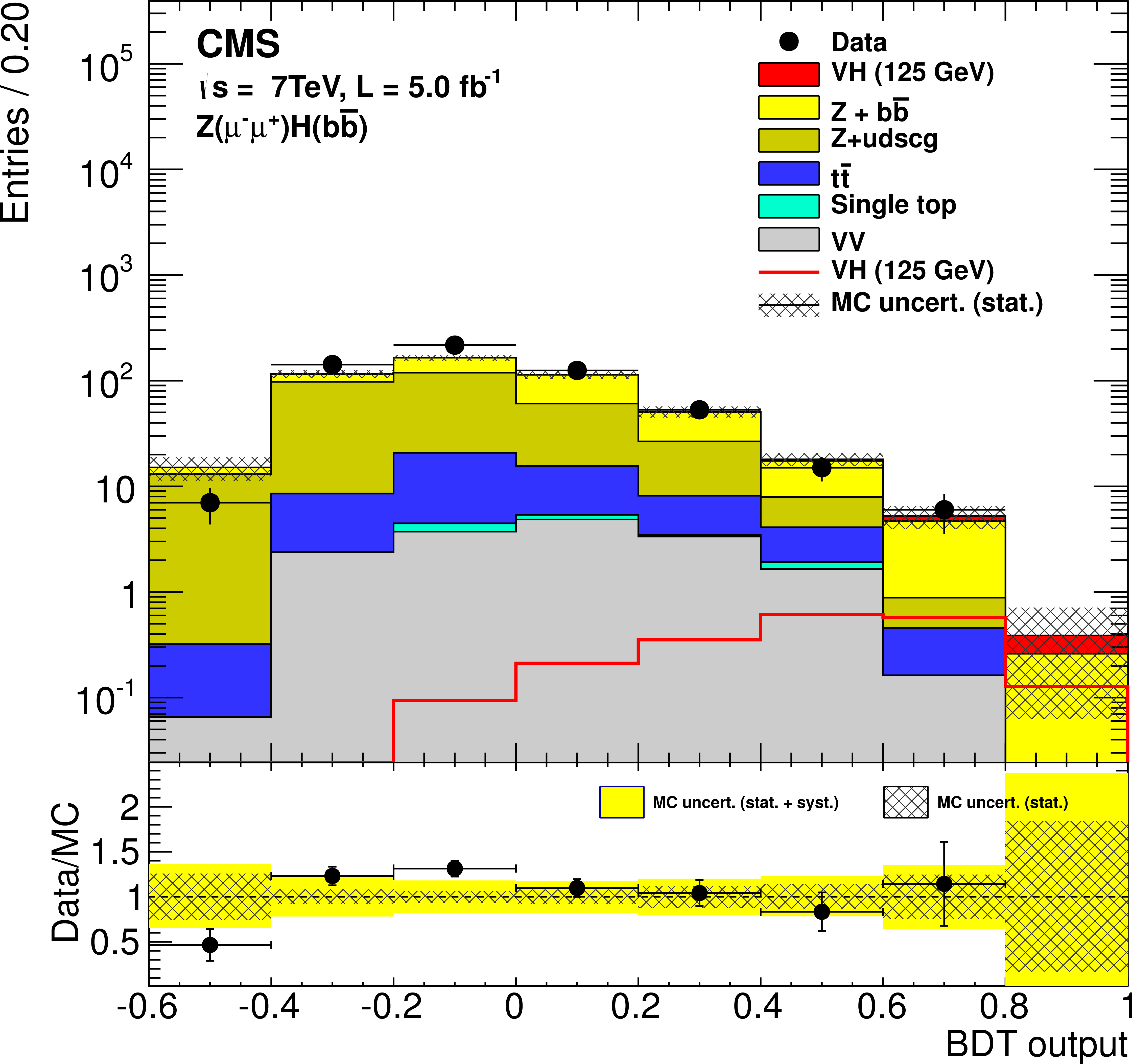
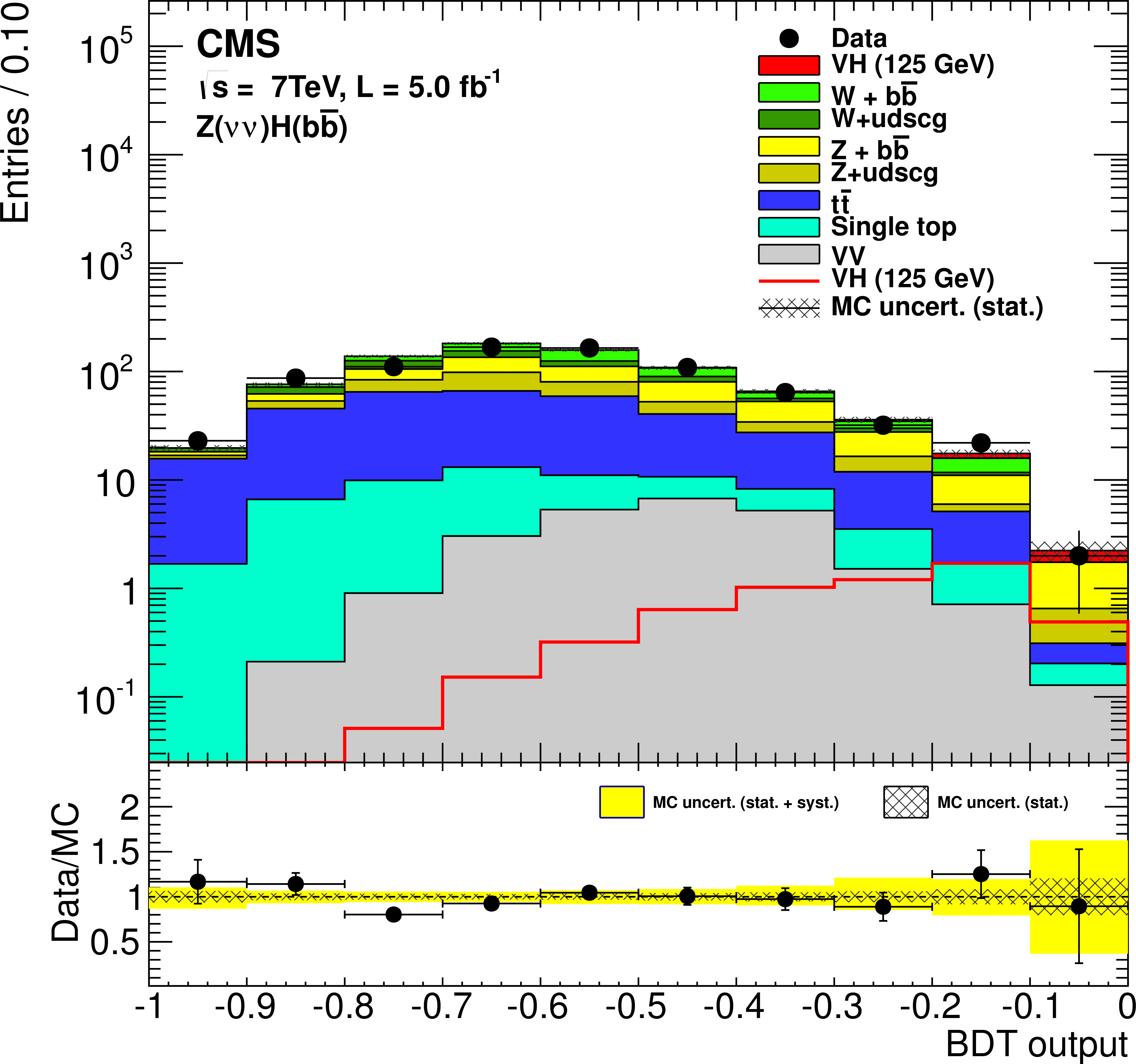
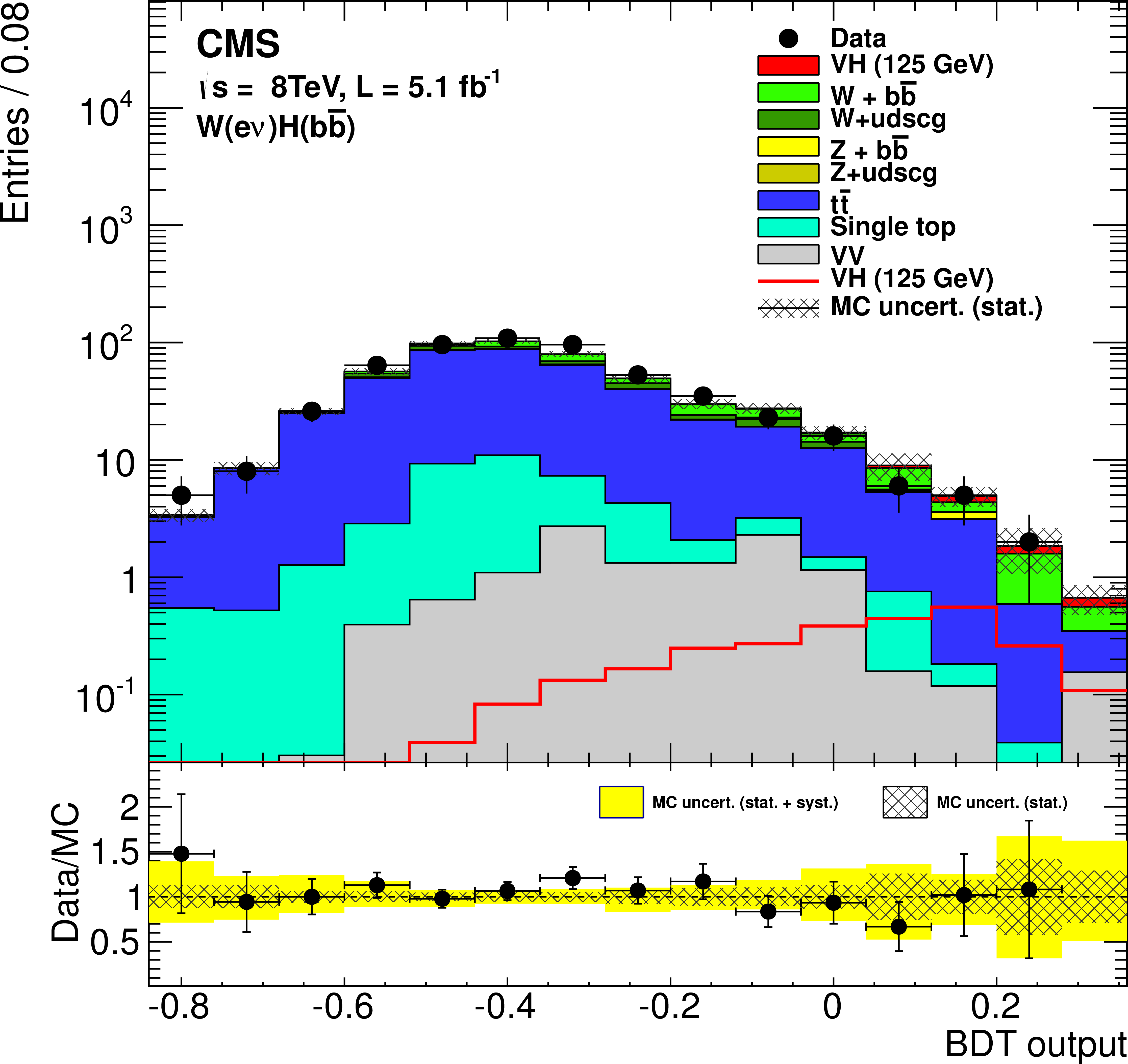
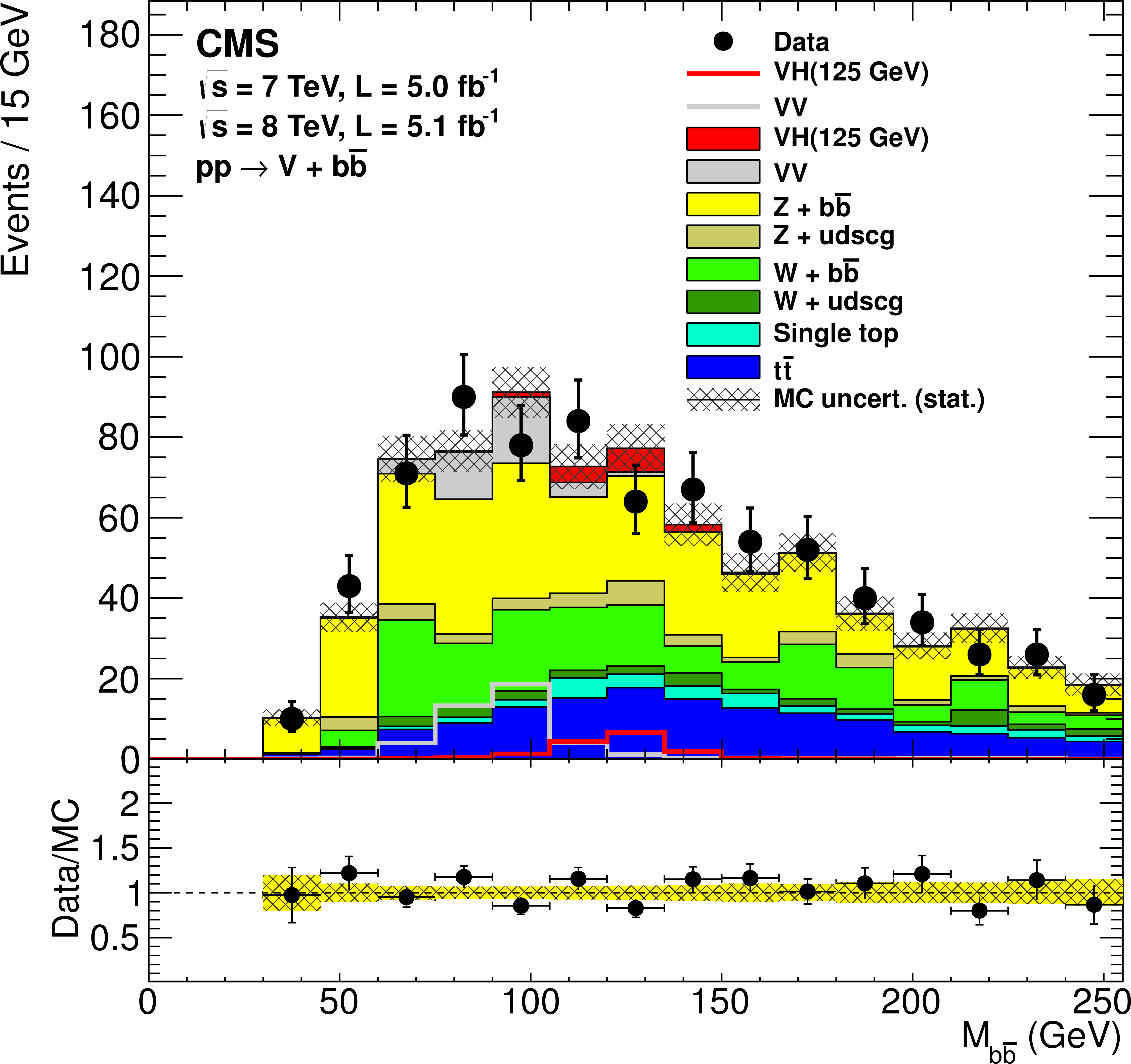
Figure 30-a:
Example of BDT output distributions in the high $ { {p_{\mathrm {T}}} (\mathrm {V})}$ bin, after all the selection criteria have been applied, for $ { {\mathrm {Z}}( {{\mu }} {{\mu }}) {\mathrm {H}} }$ (top left), $ { {\mathrm {Z}}( {\nu } {\nu }) {\mathrm {H}} }$ (top right), and $ { {\mathrm {W}}( {\mathrm {e}} {\nu }) {\mathrm {H}} }$ (bottom left). Bottom right: the $ {\mathrm {b}}$-tagged dijet invariant-mass distribution from the combination of all VH channels for the combined 7 and 8 TeV data sets. Only events that pass a more restrictive selection are included (see text). For all figures the solid histograms show the signal and the various backgrounds, with the hatched region denoting the statistical uncertainties in the MC simulation. The data are represented by points with error bars. The VH signal is represented by a red line histogram. The ratio of the data to the sum of the expected background distributions is shown at the bottom of each figure. |
png pdf |
Figure 30-b:
Example of BDT output distributions in the high $ { {p_{\mathrm {T}}} (\mathrm {V})}$ bin, after all the selection criteria have been applied, for $ { {\mathrm {Z}}( {{\mu }} {{\mu }}) {\mathrm {H}} }$ (top left), $ { {\mathrm {Z}}( {\nu } {\nu }) {\mathrm {H}} }$ (top right), and $ { {\mathrm {W}}( {\mathrm {e}} {\nu }) {\mathrm {H}} }$ (bottom left). Bottom right: the $ {\mathrm {b}}$-tagged dijet invariant-mass distribution from the combination of all VH channels for the combined 7 and 8 TeV data sets. Only events that pass a more restrictive selection are included (see text). For all figures the solid histograms show the signal and the various backgrounds, with the hatched region denoting the statistical uncertainties in the MC simulation. The data are represented by points with error bars. The VH signal is represented by a red line histogram. The ratio of the data to the sum of the expected background distributions is shown at the bottom of each figure. |
png pdf |
Figure 30-c:
Example of BDT output distributions in the high $ { {p_{\mathrm {T}}} (\mathrm {V})}$ bin, after all the selection criteria have been applied, for $ { {\mathrm {Z}}( {{\mu }} {{\mu }}) {\mathrm {H}} }$ (top left), $ { {\mathrm {Z}}( {\nu } {\nu }) {\mathrm {H}} }$ (top right), and $ { {\mathrm {W}}( {\mathrm {e}} {\nu }) {\mathrm {H}} }$ (bottom left). Bottom right: the $ {\mathrm {b}}$-tagged dijet invariant-mass distribution from the combination of all VH channels for the combined 7 and 8 TeV data sets. Only events that pass a more restrictive selection are included (see text). For all figures the solid histograms show the signal and the various backgrounds, with the hatched region denoting the statistical uncertainties in the MC simulation. The data are represented by points with error bars. The VH signal is represented by a red line histogram. The ratio of the data to the sum of the expected background distributions is shown at the bottom of each figure. |
png pdf |
Figure 30-d:
Example of BDT output distributions in the high $ { {p_{\mathrm {T}}} (\mathrm {V})}$ bin, after all the selection criteria have been applied, for $ { {\mathrm {Z}}( {{\mu }} {{\mu }}) {\mathrm {H}} }$ (top left), $ { {\mathrm {Z}}( {\nu } {\nu }) {\mathrm {H}} }$ (top right), and $ { {\mathrm {W}}( {\mathrm {e}} {\nu }) {\mathrm {H}} }$ (bottom left). Bottom right: the $ {\mathrm {b}}$-tagged dijet invariant-mass distribution from the combination of all VH channels for the combined 7 and 8 TeV data sets. Only events that pass a more restrictive selection are included (see text). For all figures the solid histograms show the signal and the various backgrounds, with the hatched region denoting the statistical uncertainties in the MC simulation. The data are represented by points with error bars. The VH signal is represented by a red line histogram. The ratio of the data to the sum of the expected background distributions is shown at the bottom of each figure. |

png pdf |
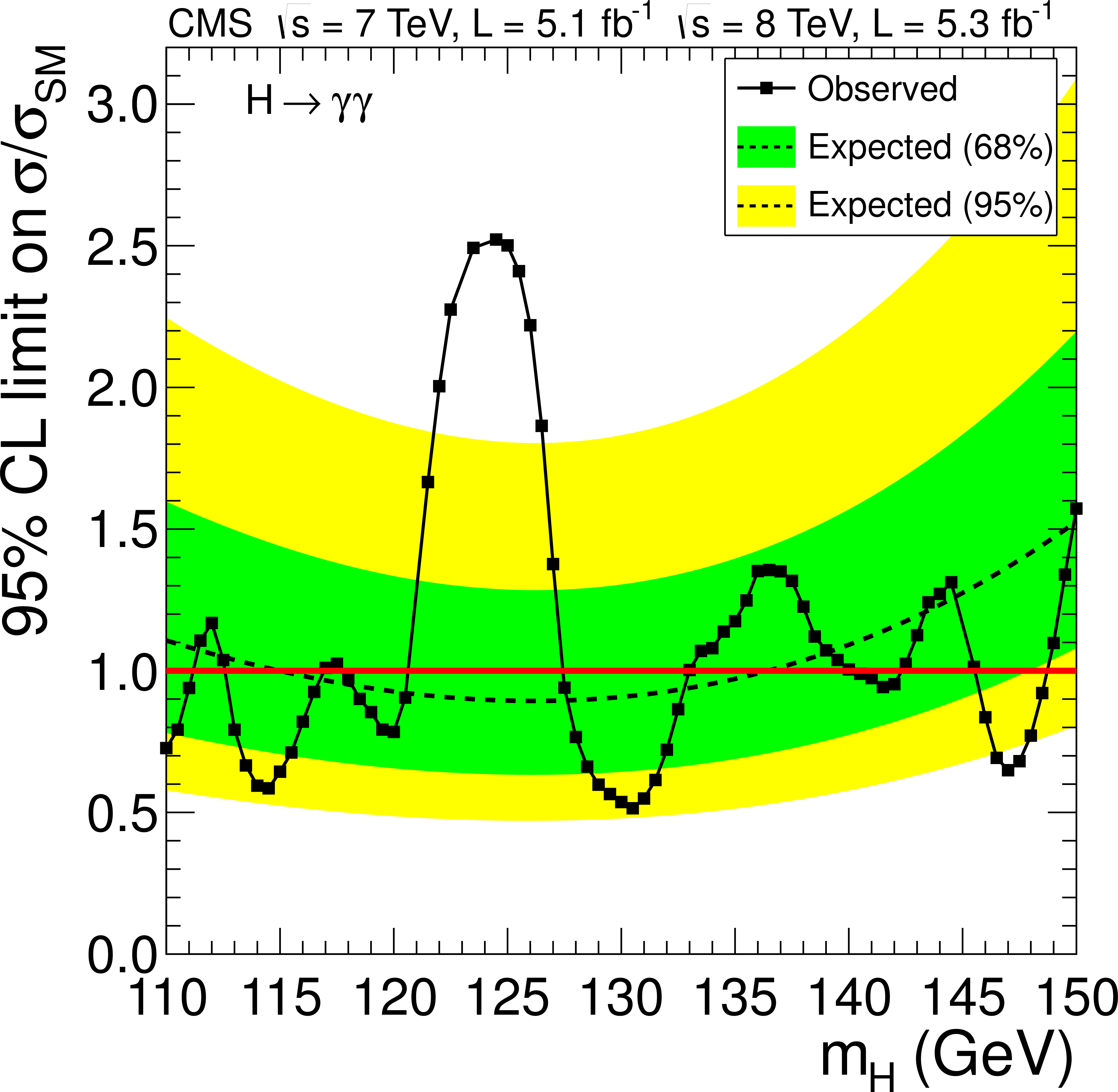
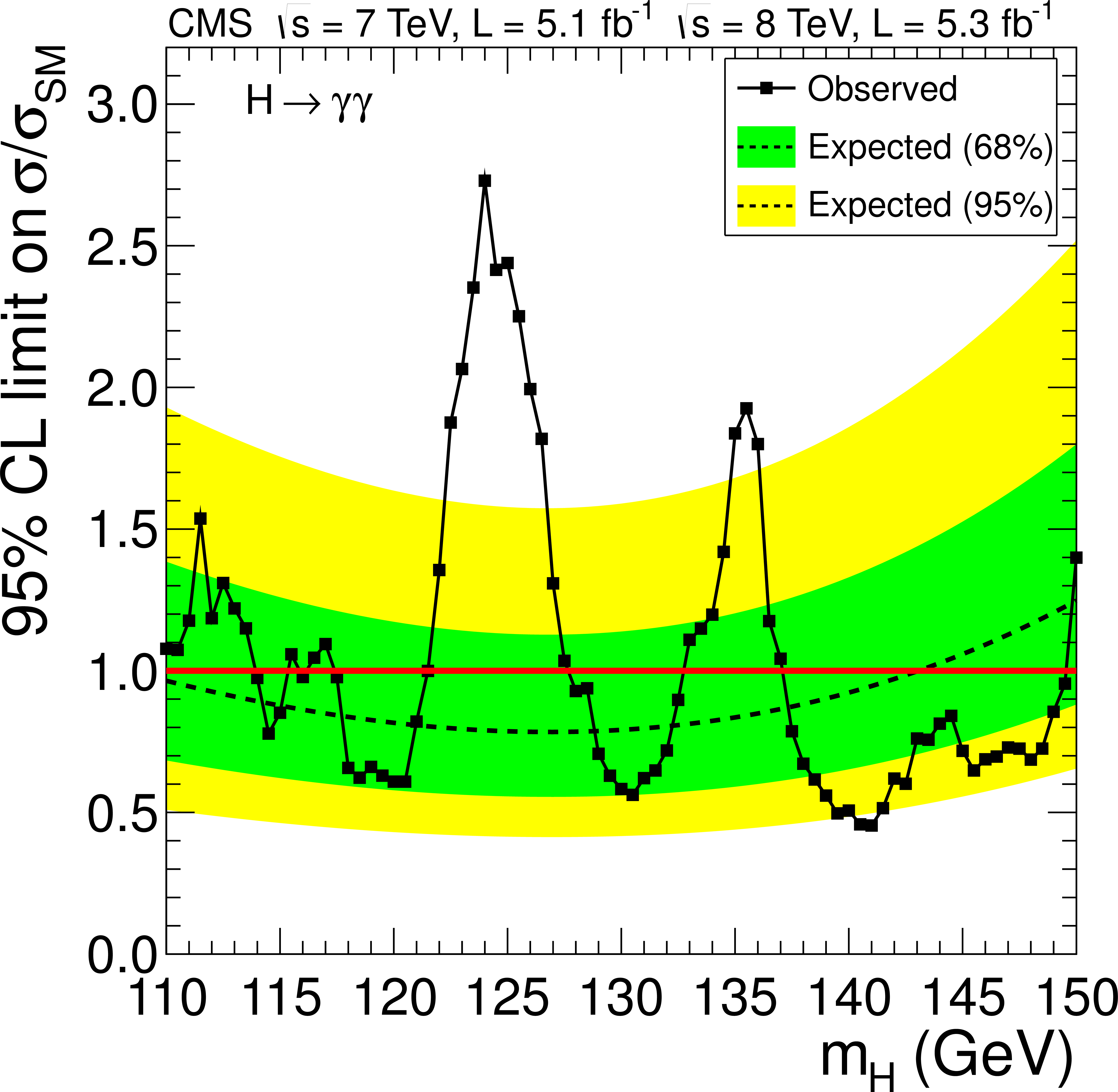
Figure 31-a:
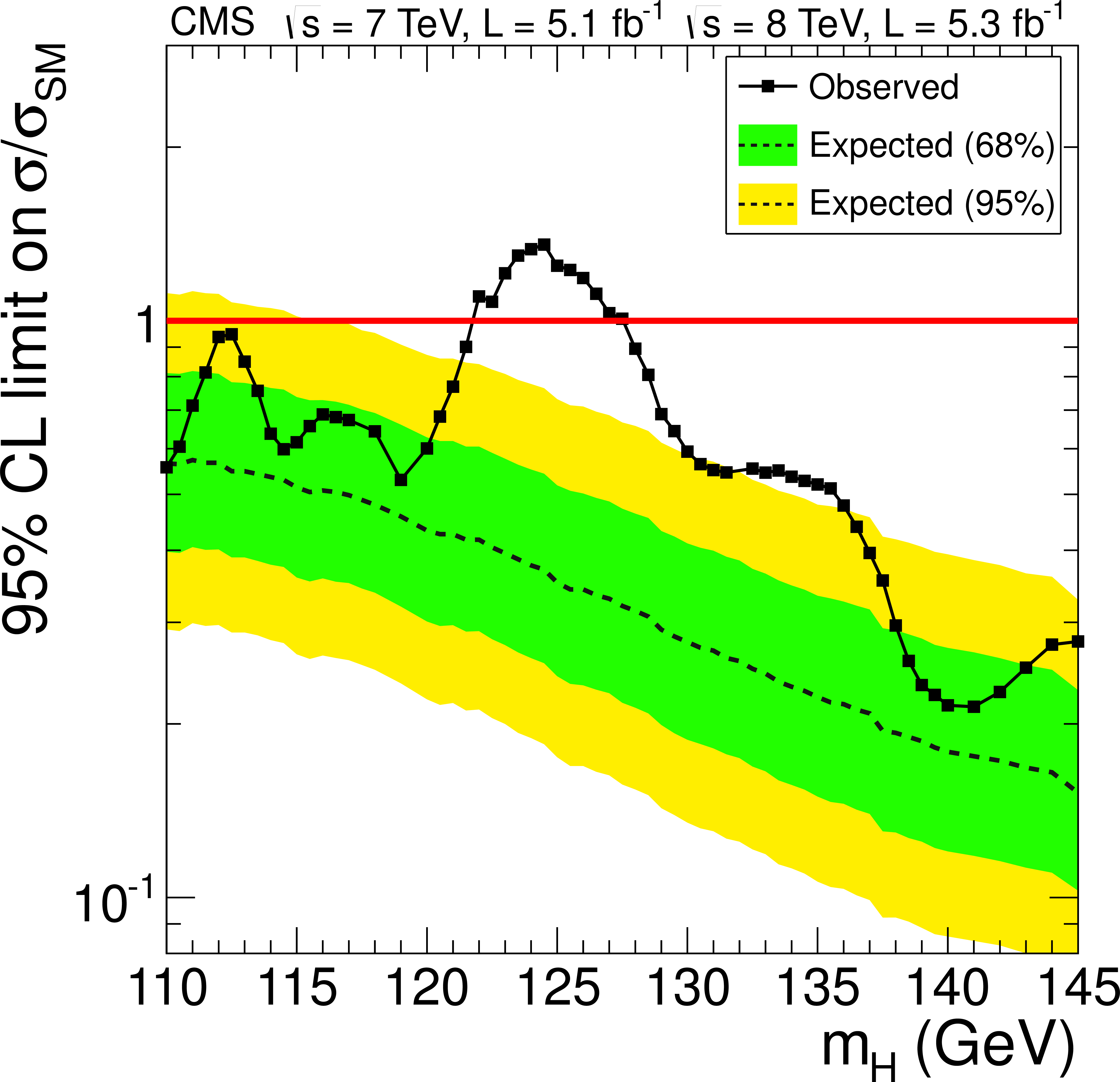
The 95% CL upper limits on the production cross section of a Higgs boson expressed in units of the SM Higgs boson production cross section, $\sigma / \sigma _\text {SM}$, as obtained in the $ {\mathrm {H}} \to {\gamma } {\gamma }$ search channel for (top) the baseline analysis, (lower left) the cut-based analysis, and (lower right) the sideband analysis. The solid lines represent the observed limits; the background-only hypotheses are represented by their median (dashed lines) and by their 68% (dark) and 95% (light) CL bands. |
png pdf |
Figure 31-b:
The 95% CL upper limits on the production cross section of a Higgs boson expressed in units of the SM Higgs boson production cross section, $\sigma / \sigma _\text {SM}$, as obtained in the $ {\mathrm {H}} \to {\gamma } {\gamma }$ search channel for (top) the baseline analysis, (lower left) the cut-based analysis, and (lower right) the sideband analysis. The solid lines represent the observed limits; the background-only hypotheses are represented by their median (dashed lines) and by their 68% (dark) and 95% (light) CL bands. |
png pdf |
Figure 31-c:
The 95% CL upper limits on the production cross section of a Higgs boson expressed in units of the SM Higgs boson production cross section, $\sigma / \sigma _\text {SM}$, as obtained in the $ {\mathrm {H}} \to {\gamma } {\gamma }$ search channel for (top) the baseline analysis, (lower left) the cut-based analysis, and (lower right) the sideband analysis. The solid lines represent the observed limits; the background-only hypotheses are represented by their median (dashed lines) and by their 68% (dark) and 95% (light) CL bands. |
png pdf |
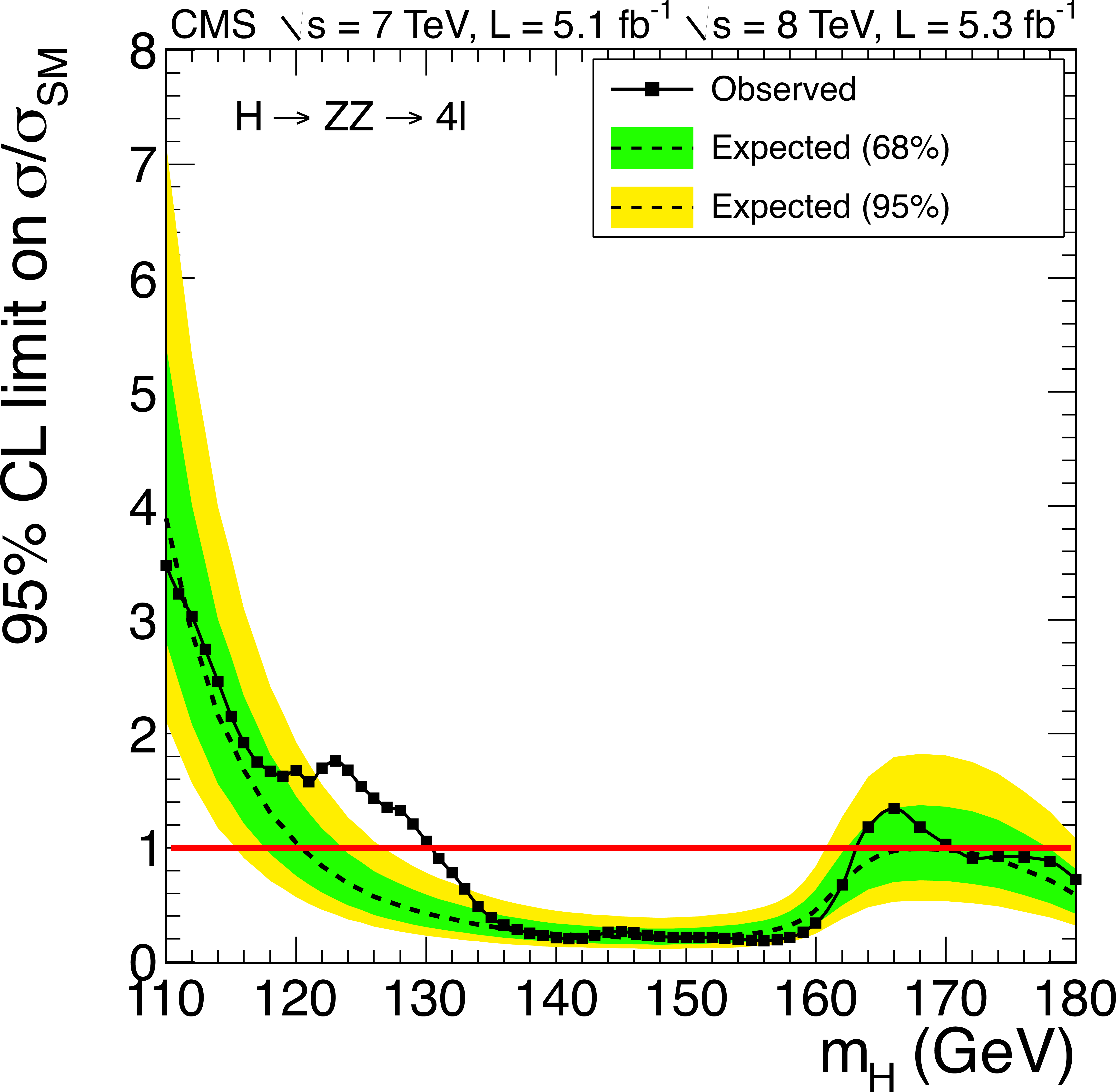
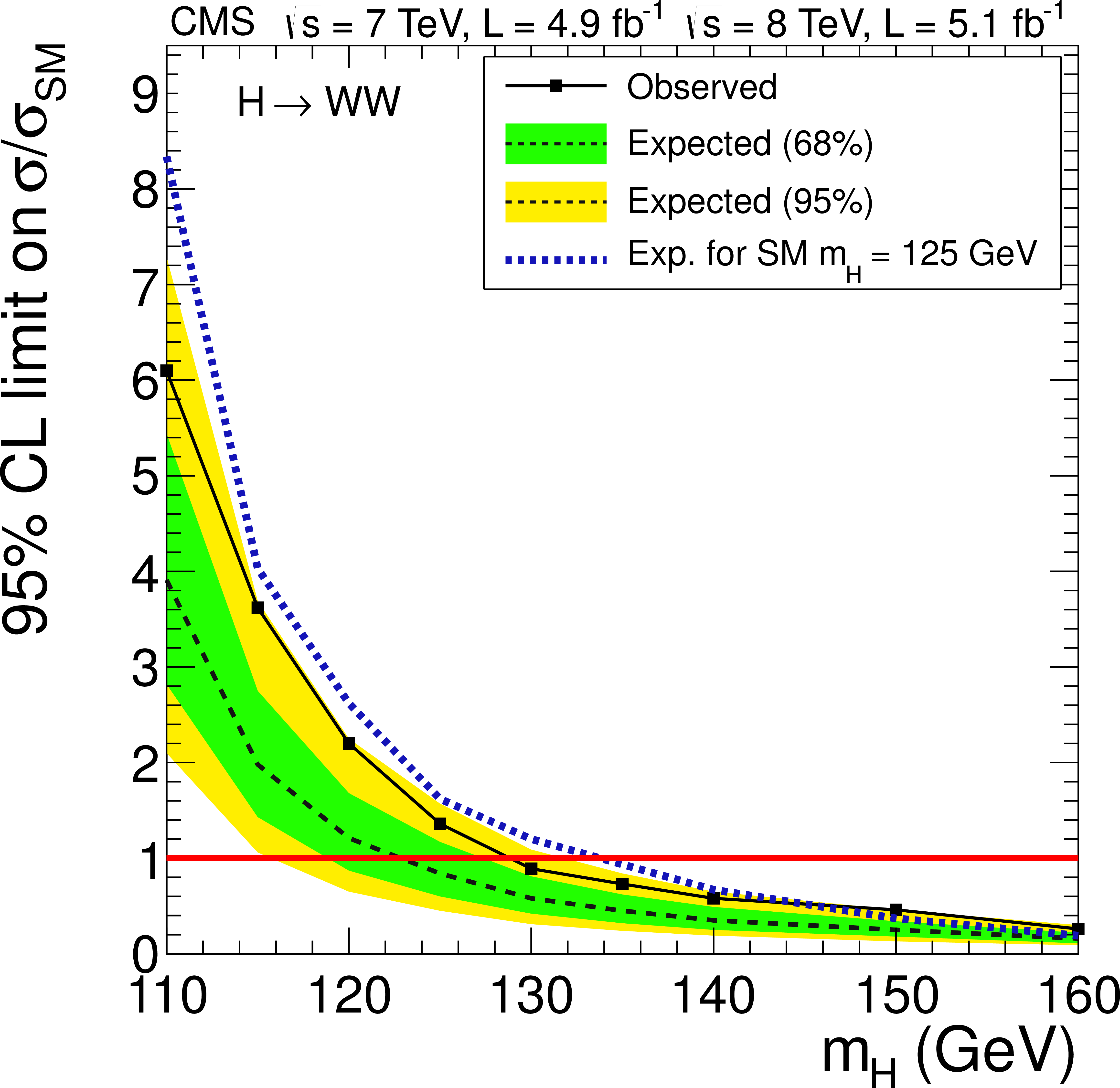
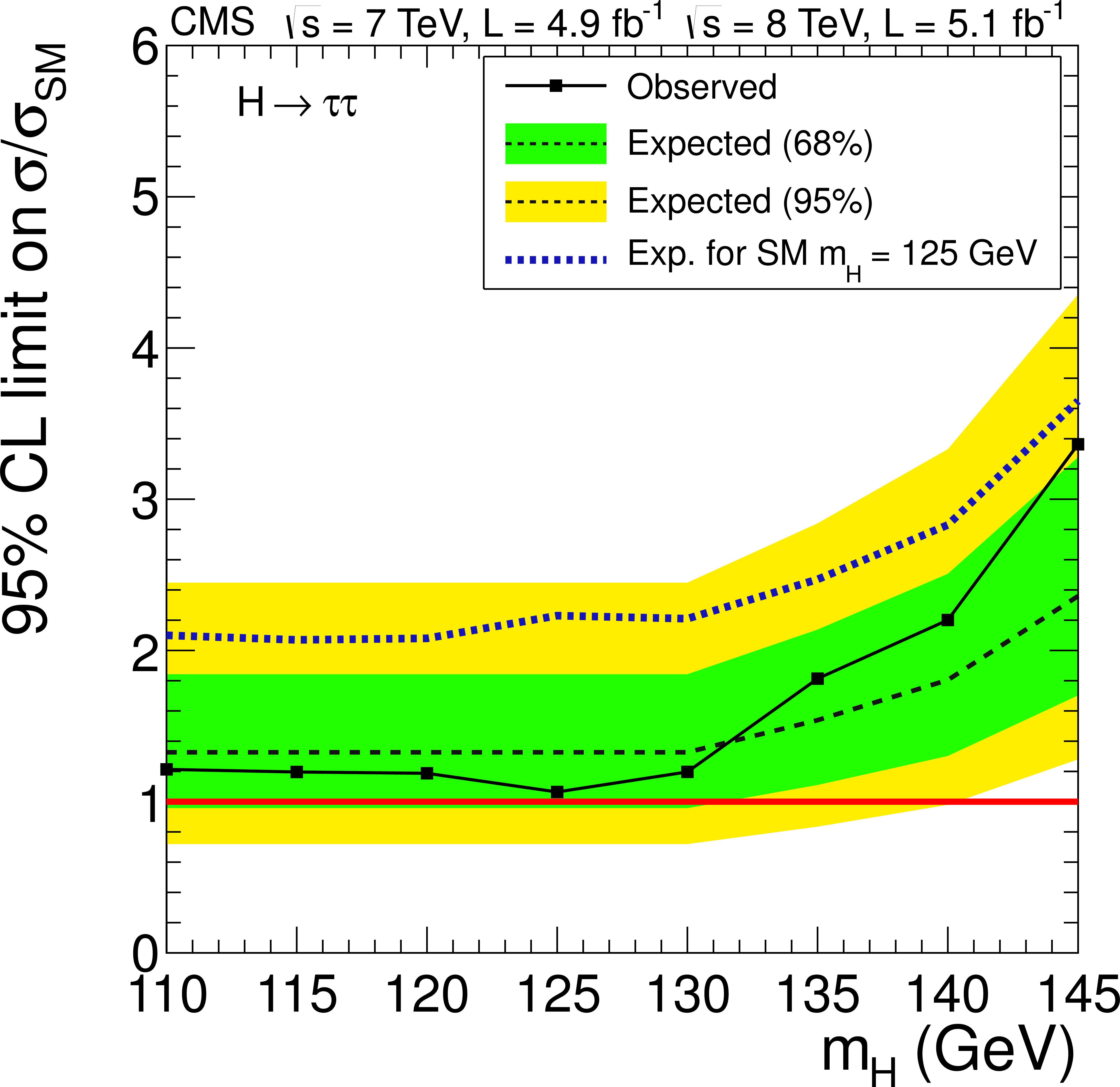
Figure 32-a:
The 95% CL upper limits on the production cross section of a Higgs boson expressed in units of the SM Higgs boson production cross section, $\sigma / \sigma _\text {SM}$, for the following search modes: (upper left) $ {\mathrm {H}} \to {\mathrm {Z}} {\mathrm {Z}}\to 4\ell $, (upper right) $ {\mathrm {H}} \to {\mathrm {W}} {\mathrm {W}}$, (lower left) $ {\mathrm {H}} \to {\tau } {\tau }$, and (lower right) $ {\mathrm {H}} \to {\mathrm {b}} {\mathrm {b}}$. The solid lines represent the observed limits; the background-only hypotheses are represented by their median (dashed lines) and by the 68% and 95% CL bands. The signal-plus-background expectation (dotted lines) from a Higgs boson with mass $ {m_{ {\mathrm {H}} }}= 125$ GeV is also shown for the final states with a poor mass resolution, $ {\mathrm {W}} {\mathrm {W}}$, $\tau \tau $, and $ {\mathrm {b}} {\mathrm {b}}$. |
png pdf |
Figure 32-b:
The 95% CL upper limits on the production cross section of a Higgs boson expressed in units of the SM Higgs boson production cross section, $\sigma / \sigma _\text {SM}$, for the following search modes: (upper left) $ {\mathrm {H}} \to {\mathrm {Z}} {\mathrm {Z}}\to 4\ell $, (upper right) $ {\mathrm {H}} \to {\mathrm {W}} {\mathrm {W}}$, (lower left) $ {\mathrm {H}} \to {\tau } {\tau }$, and (lower right) $ {\mathrm {H}} \to {\mathrm {b}} {\mathrm {b}}$. The solid lines represent the observed limits; the background-only hypotheses are represented by their median (dashed lines) and by the 68% and 95% CL bands. The signal-plus-background expectation (dotted lines) from a Higgs boson with mass $ {m_{ {\mathrm {H}} }}= 125$ GeV is also shown for the final states with a poor mass resolution, $ {\mathrm {W}} {\mathrm {W}}$, $\tau \tau $, and $ {\mathrm {b}} {\mathrm {b}}$. |
png pdf |
Figure 32-c:
The 95% CL upper limits on the production cross section of a Higgs boson expressed in units of the SM Higgs boson production cross section, $\sigma / \sigma _\text {SM}$, for the following search modes: (upper left) $ {\mathrm {H}} \to {\mathrm {Z}} {\mathrm {Z}}\to 4\ell $, (upper right) $ {\mathrm {H}} \to {\mathrm {W}} {\mathrm {W}}$, (lower left) $ {\mathrm {H}} \to {\tau } {\tau }$, and (lower right) $ {\mathrm {H}} \to {\mathrm {b}} {\mathrm {b}}$. The solid lines represent the observed limits; the background-only hypotheses are represented by their median (dashed lines) and by the 68% and 95% CL bands. The signal-plus-background expectation (dotted lines) from a Higgs boson with mass $ {m_{ {\mathrm {H}} }}= 125$ GeV is also shown for the final states with a poor mass resolution, $ {\mathrm {W}} {\mathrm {W}}$, $\tau \tau $, and $ {\mathrm {b}} {\mathrm {b}}$. |

png pdf |
Figure 32-d:
The 95% CL upper limits on the production cross section of a Higgs boson expressed in units of the SM Higgs boson production cross section, $\sigma / \sigma _\text {SM}$, for the following search modes: (upper left) $ {\mathrm {H}} \to {\mathrm {Z}} {\mathrm {Z}}\to 4\ell $, (upper right) $ {\mathrm {H}} \to {\mathrm {W}} {\mathrm {W}}$, (lower left) $ {\mathrm {H}} \to {\tau } {\tau }$, and (lower right) $ {\mathrm {H}} \to {\mathrm {b}} {\mathrm {b}}$. The solid lines represent the observed limits; the background-only hypotheses are represented by their median (dashed lines) and by the 68% and 95% CL bands. The signal-plus-background expectation (dotted lines) from a Higgs boson with mass $ {m_{ {\mathrm {H}} }}= 125$ GeV is also shown for the final states with a poor mass resolution, $ {\mathrm {W}} {\mathrm {W}}$, $\tau \tau $, and $ {\mathrm {b}} {\mathrm {b}}$. |
png pdf |
Figure 33-a:
The 95% CL upper limits on the production cross section of a Higgs boson expressed in units of the SM Higgs boson production cross section, $\sigma / \sigma _\text {SM}$, (left) and the $ {\mathrm {CL_s} }$ values (right) for the SM Higgs boson hypothesis, as a function of the Higgs boson mass for the five decay modes and the 7 and 8 TeV data sample combined. The solid lines represent the observed limits; the background-only hypotheses are represented by their median (dashed lines) and by the 68% and 95% CL bands. The three horizontal lines on the right plot show the $ {\mathrm {CL_s} }$ values 0.05, 0.01, and 0.001, corresponding to 95%, 99%, and 99.9% confidence levels, defined as $(1- {\mathrm {CL_s} })$. |

png pdf |
Figure 33-b:
The 95% CL upper limits on the production cross section of a Higgs boson expressed in units of the SM Higgs boson production cross section, $\sigma / \sigma _\text {SM}$, (left) and the $ {\mathrm {CL_s} }$ values (right) for the SM Higgs boson hypothesis, as a function of the Higgs boson mass for the five decay modes and the 7 and 8 TeV data sample combined. The solid lines represent the observed limits; the background-only hypotheses are represented by their median (dashed lines) and by the 68% and 95% CL bands. The three horizontal lines on the right plot show the $ {\mathrm {CL_s} }$ values 0.05, 0.01, and 0.001, corresponding to 95%, 99%, and 99.9% confidence levels, defined as $(1- {\mathrm {CL_s} })$. |
png pdf |
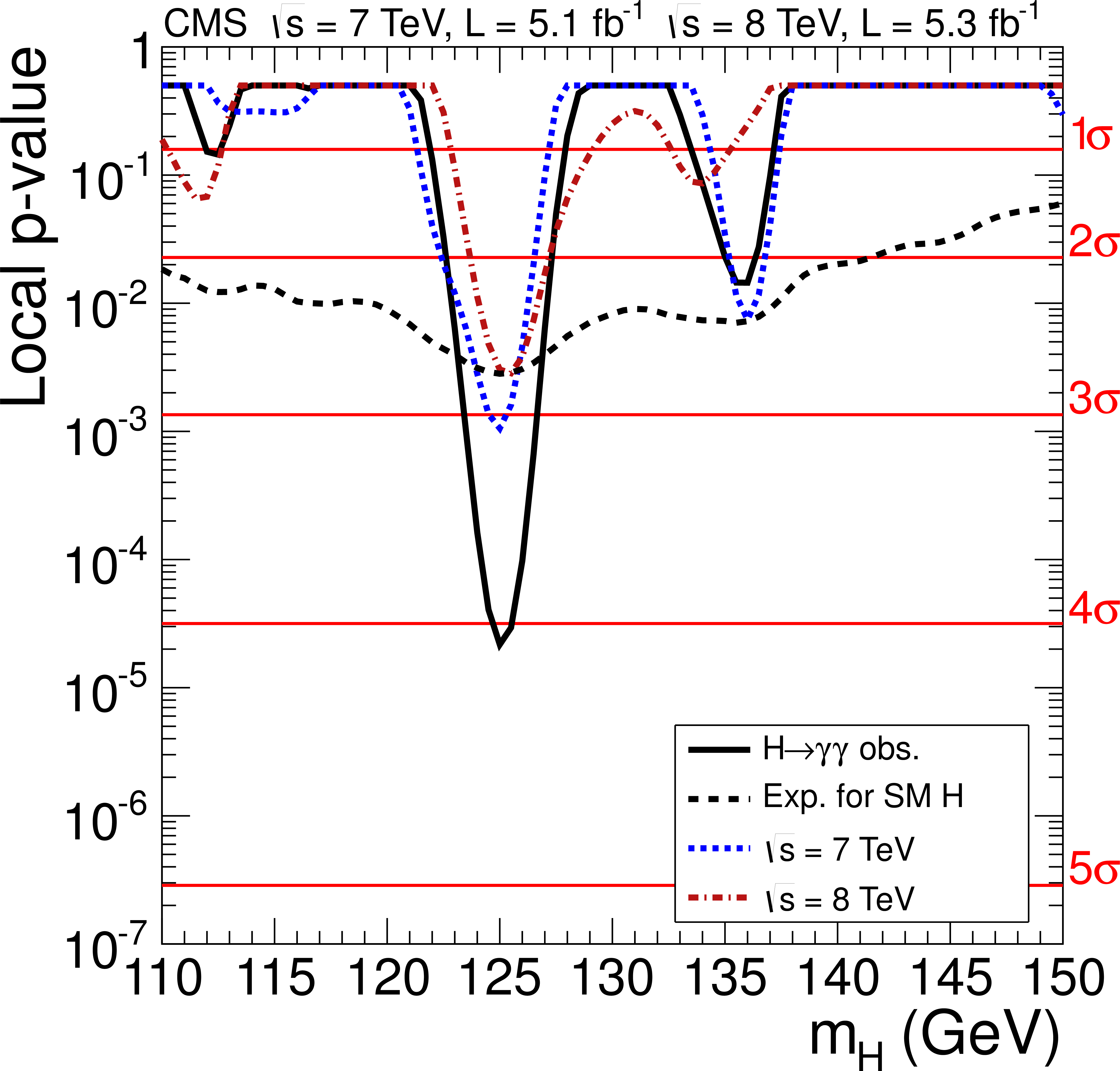
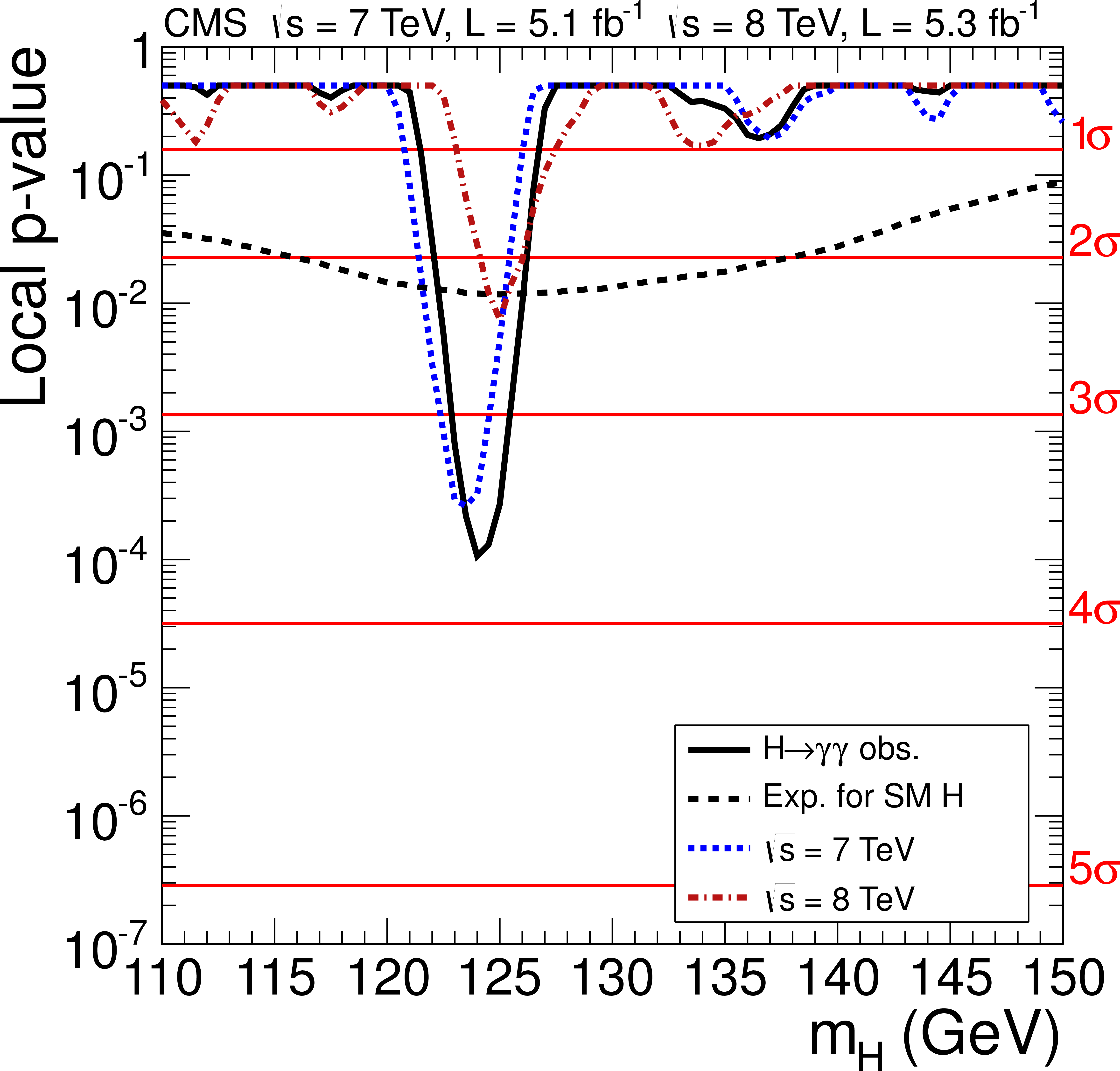
Figure 34-a:
The local $p$-value as a function of $ {m_{ {\mathrm {H}} }}$ for the 7 and 8 TeV data sets and their combination for the $ {\gamma } {\gamma }$ mode from (top) the primary analysis, (lower left) the cut-based analysis, and (lower right) the side-band analysis. The observed $p$-values for the combined 7 and 8 TeV data sets are shown by the solid lines; the median expected $p$-values for a SM Higgs boson with mass $ {m_{ {\mathrm {H}} }}$, are shown by the dashed lines. The horizontal lines show the relationship between the $p$-value (left $y$ axis) and the significance in standard deviations (right $y$ axis). |
png pdf |
Figure 34-b:
The local $p$-value as a function of $ {m_{ {\mathrm {H}} }}$ for the 7 and 8 TeV data sets and their combination for the $ {\gamma } {\gamma }$ mode from (top) the primary analysis, (lower left) the cut-based analysis, and (lower right) the side-band analysis. The observed $p$-values for the combined 7 and 8 TeV data sets are shown by the solid lines; the median expected $p$-values for a SM Higgs boson with mass $ {m_{ {\mathrm {H}} }}$, are shown by the dashed lines. The horizontal lines show the relationship between the $p$-value (left $y$ axis) and the significance in standard deviations (right $y$ axis). |

png pdf |
Figure 34-c:
The local $p$-value as a function of $ {m_{ {\mathrm {H}} }}$ for the 7 and 8 TeV data sets and their combination for the $ {\gamma } {\gamma }$ mode from (top) the primary analysis, (lower left) the cut-based analysis, and (lower right) the side-band analysis. The observed $p$-values for the combined 7 and 8 TeV data sets are shown by the solid lines; the median expected $p$-values for a SM Higgs boson with mass $ {m_{ {\mathrm {H}} }}$, are shown by the dashed lines. The horizontal lines show the relationship between the $p$-value (left $y$ axis) and the significance in standard deviations (right $y$ axis). |
png pdf |
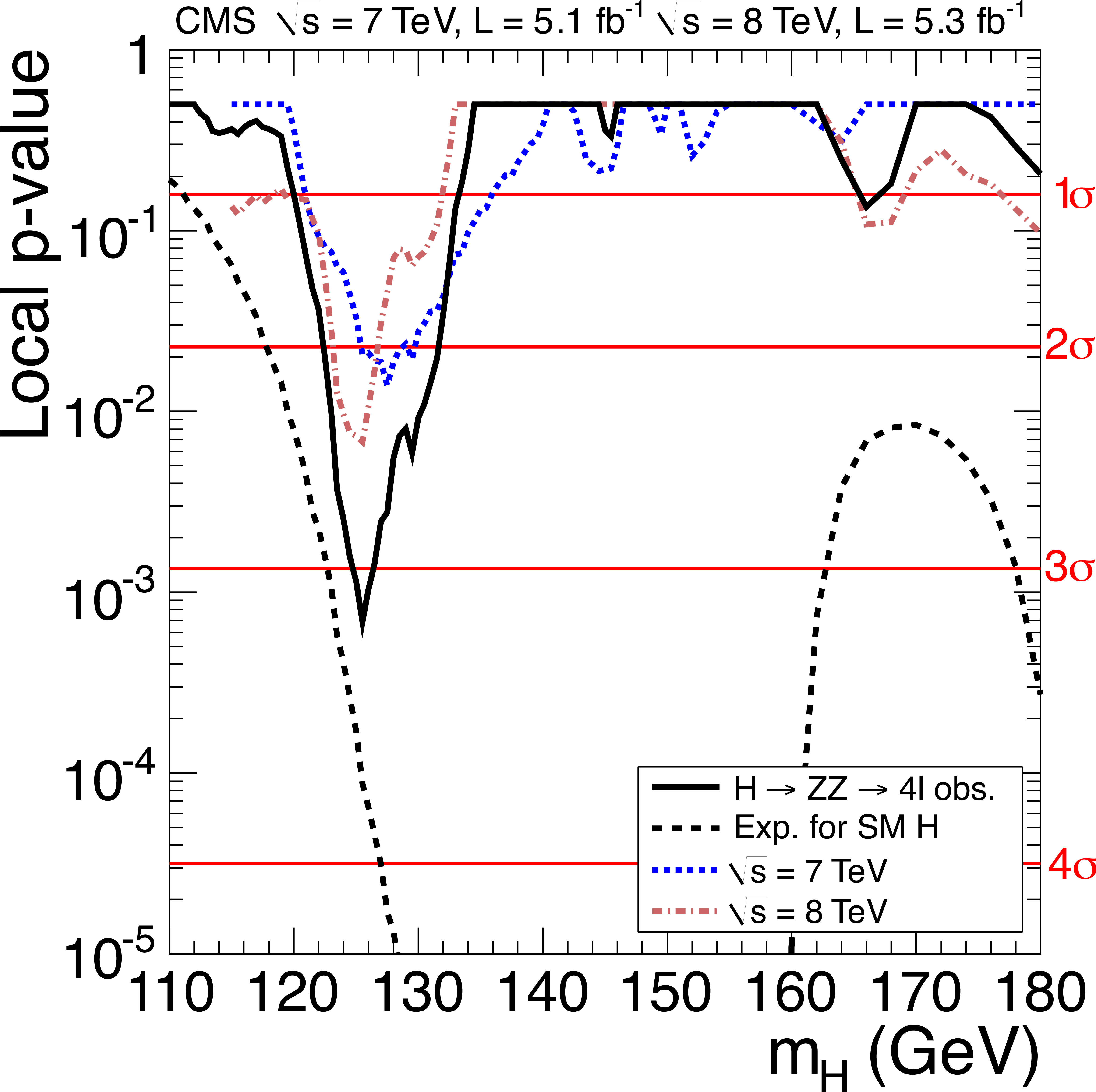
Figure 35:
The local $p$-value as a function of $ {m_{ {\mathrm {H}} }}$ for the 7 and 8 TeV data sets and their combination for the $ {\mathrm {Z}} {\mathrm {Z}}\to 4\ell $ channel. The observed $p$-values for the combined 7 and 8 TeV data sets are shown by the solid line; the median expected $p$-values for a SM Higgs boson with mass $ {m_{ {\mathrm {H}} }}$ are shown by the dashed line. The observed $p$-values for the 7 and 8 TeV data sets are shown by the dotted lines. The horizontal lines show the relationship between the $p$-value (left $y$ axis) and the significance in standard deviations (right $y$ axis). |
png pdf |
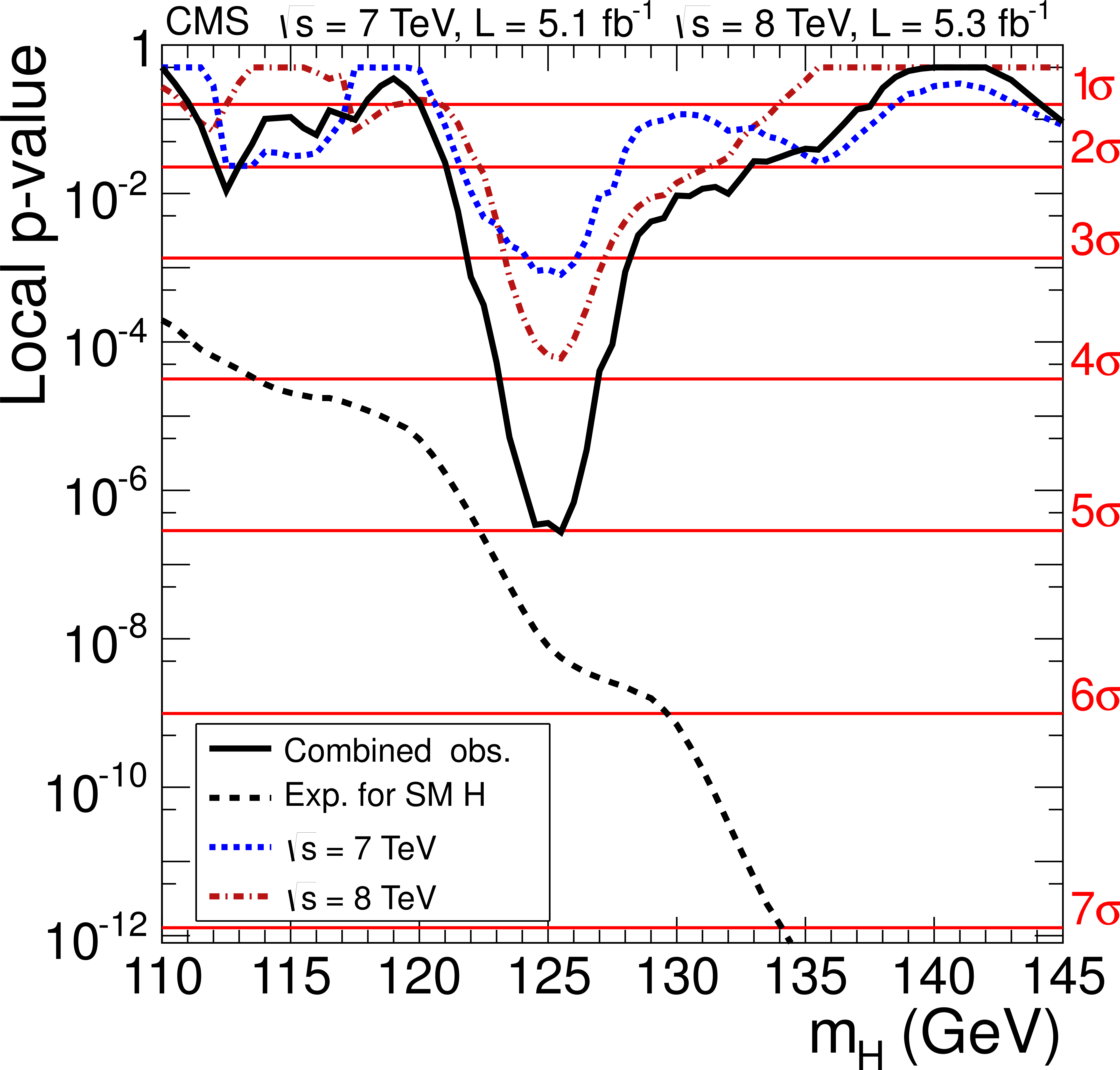
Figure 36-a:
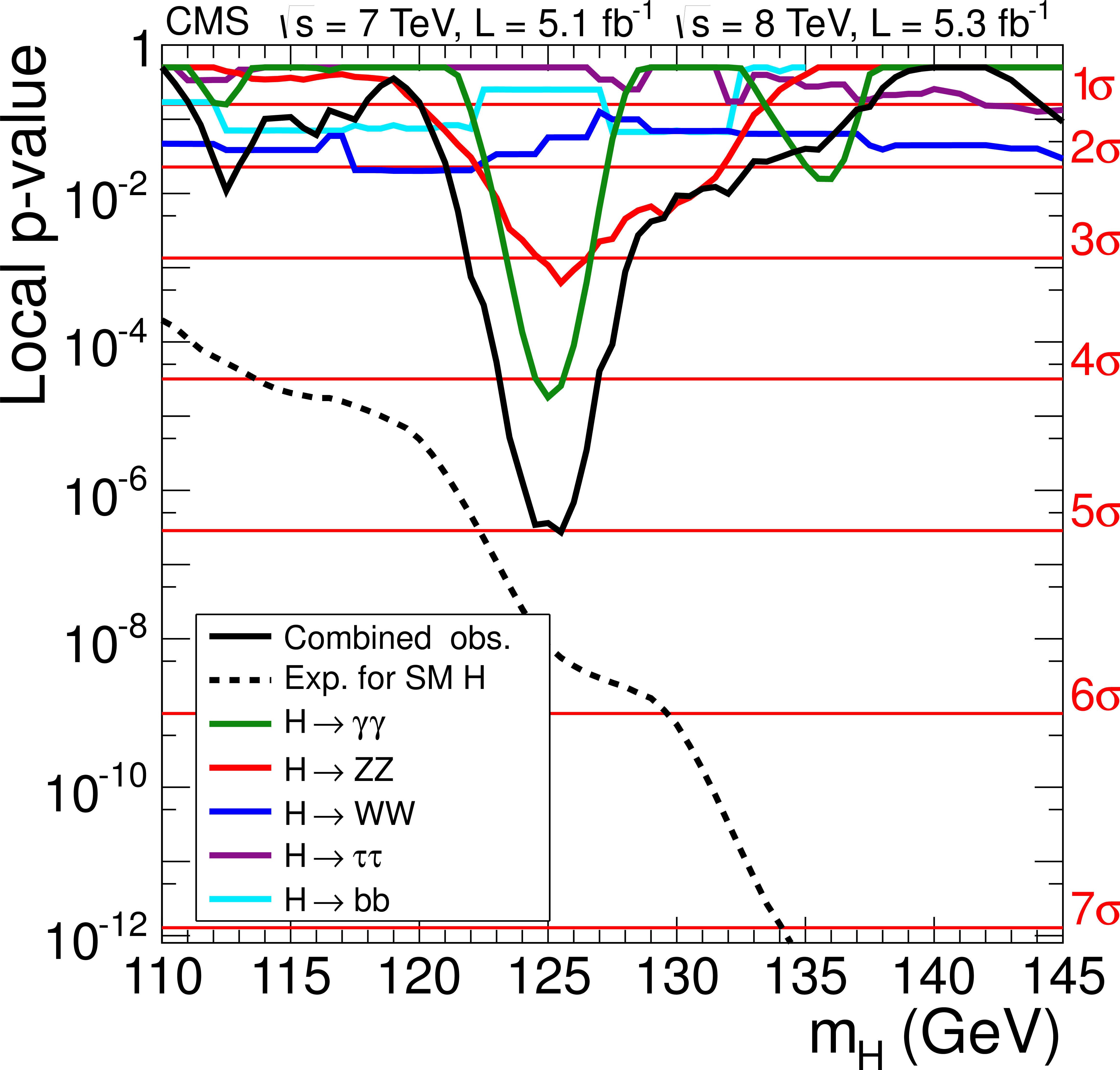
(Left) The observed local $p$-value for the combination of all five decay modes with the 7 and 8 TeV data sets, and their combination as a function of the Higgs boson mass. (Right) The observed local $p$-value for each separate decay mode and their combination, as a function of the Higgs boson mass. The dashed lines show the mean expected local $p$-values for a SM Higgs boson with mass $ {m_{ {\mathrm {H}} }}$. |
png pdf |
Figure 36-b:
(Left) The observed local $p$-value for the combination of all five decay modes with the 7 and 8 TeV data sets, and their combination as a function of the Higgs boson mass. (Right) The observed local $p$-value for each separate decay mode and their combination, as a function of the Higgs boson mass. The dashed lines show the mean expected local $p$-values for a SM Higgs boson with mass $ {m_{ {\mathrm {H}} }}$. |
png pdf |
Figure 37-a:
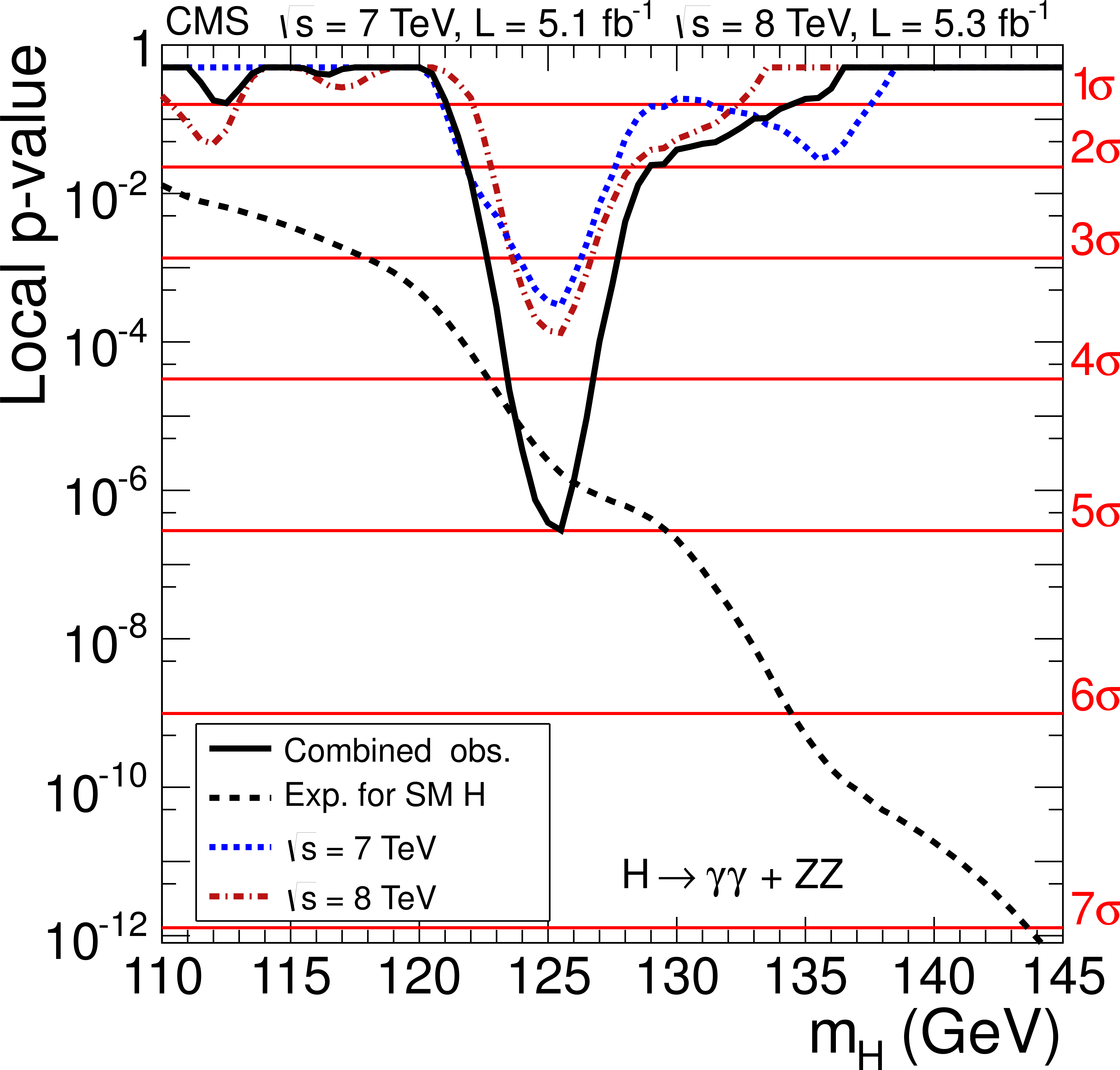
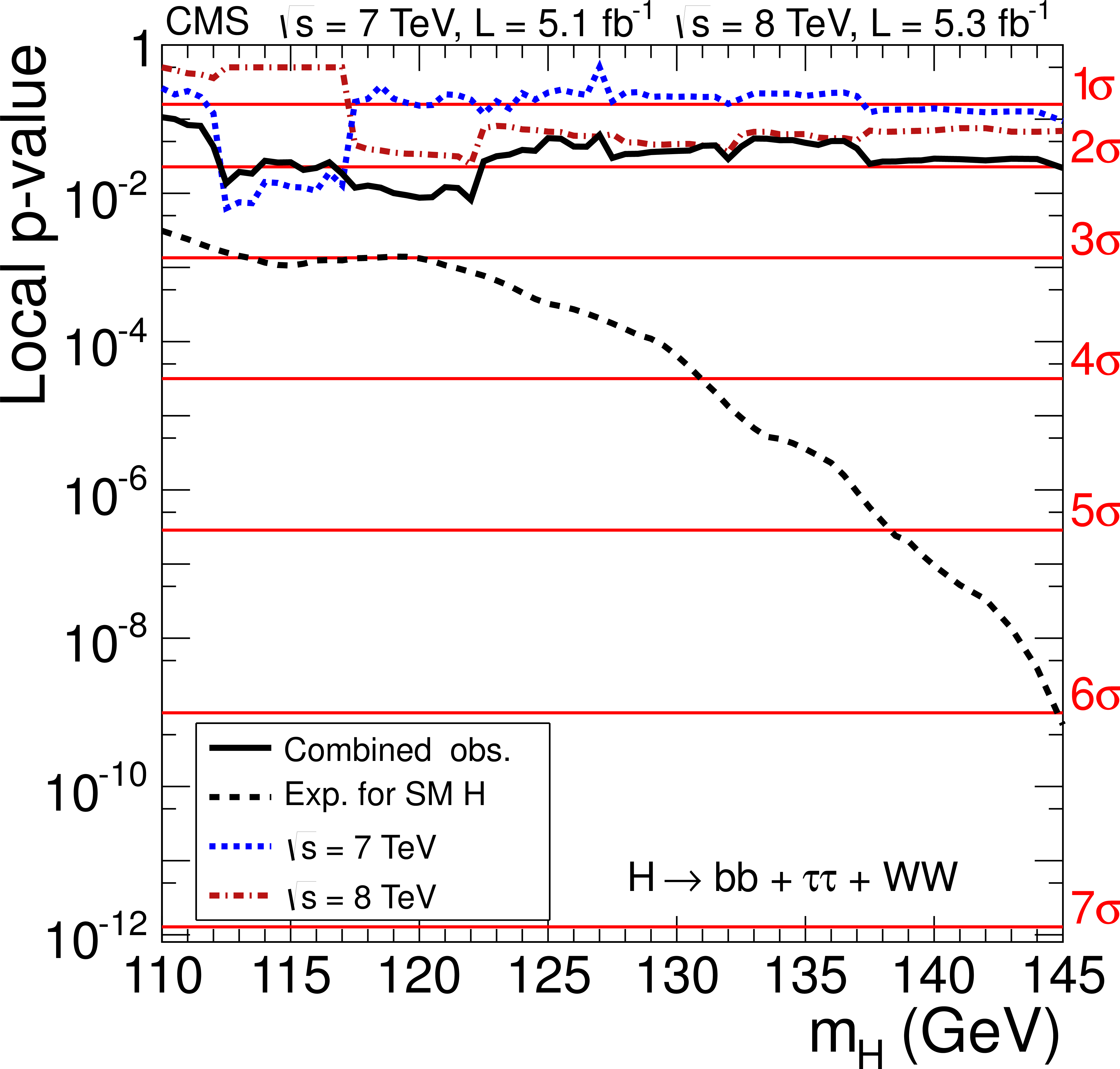
The observed local $p$-value for the $ {\gamma } {\gamma }$ and $ {\mathrm {Z}} {\mathrm {Z}}\to 4\ell $ decay channels with good mass resolution (left) and the $ {\mathrm {W}} {\mathrm {W}}$, $ {\mathrm {b}} {\mathrm {b}}$, and $ {\tau } {\tau }$ modes with poorer mass resolution (right), as a function of the Higgs boson mass for the 7 and 8 TeV data sets and their combination. The dashed lines show the expected local $p$-values for a SM Higgs boson with mass $ {m_{ {\mathrm {H}} }}$. |
png pdf |
Figure 37-b:
The observed local $p$-value for the $ {\gamma } {\gamma }$ and $ {\mathrm {Z}} {\mathrm {Z}}\to 4\ell $ decay channels with good mass resolution (left) and the $ {\mathrm {W}} {\mathrm {W}}$, $ {\mathrm {b}} {\mathrm {b}}$, and $ {\tau } {\tau }$ modes with poorer mass resolution (right), as a function of the Higgs boson mass for the 7 and 8 TeV data sets and their combination. The dashed lines show the expected local $p$-values for a SM Higgs boson with mass $ {m_{ {\mathrm {H}} }}$. |
png pdf |
Figure 38-a:
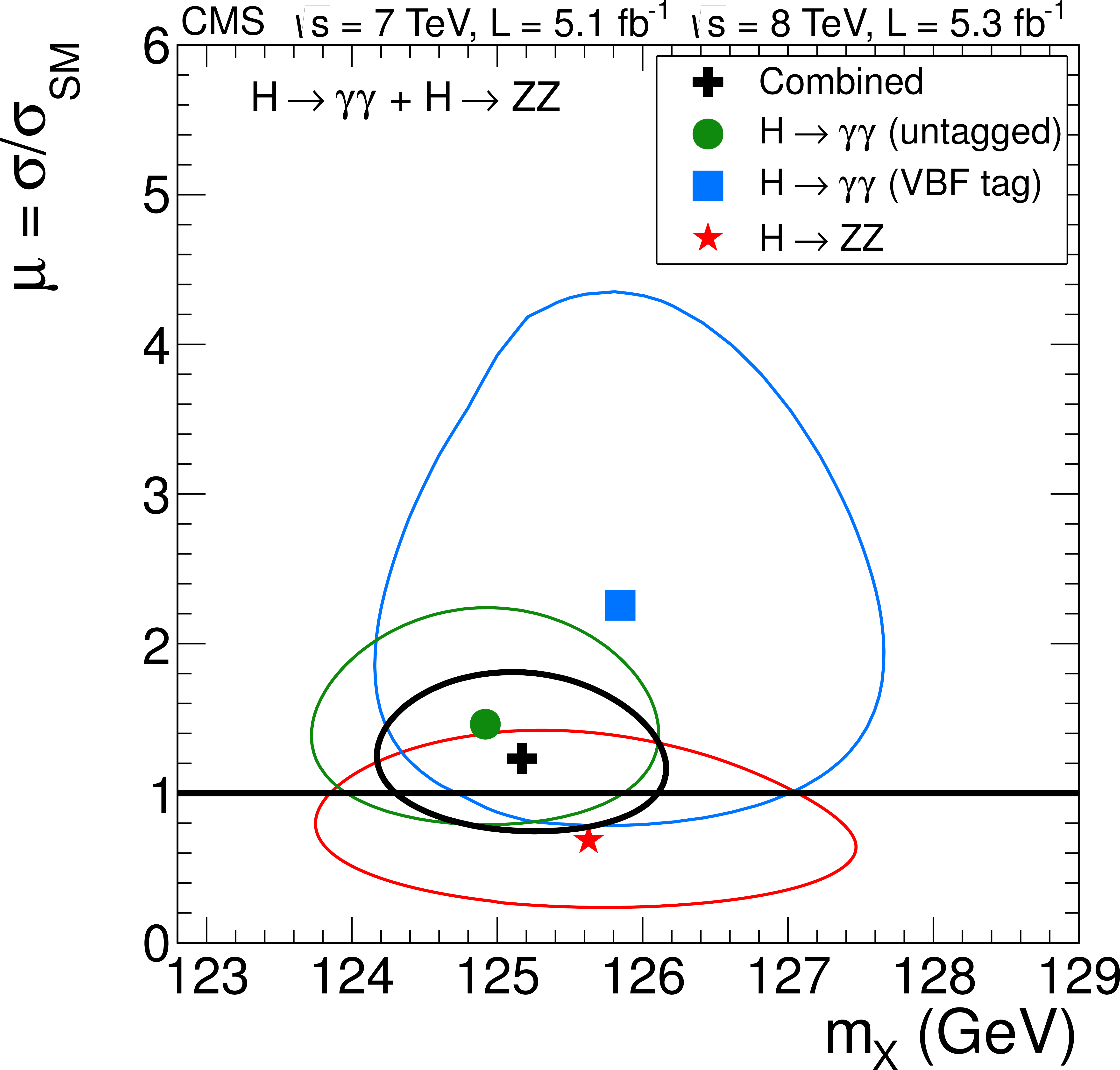
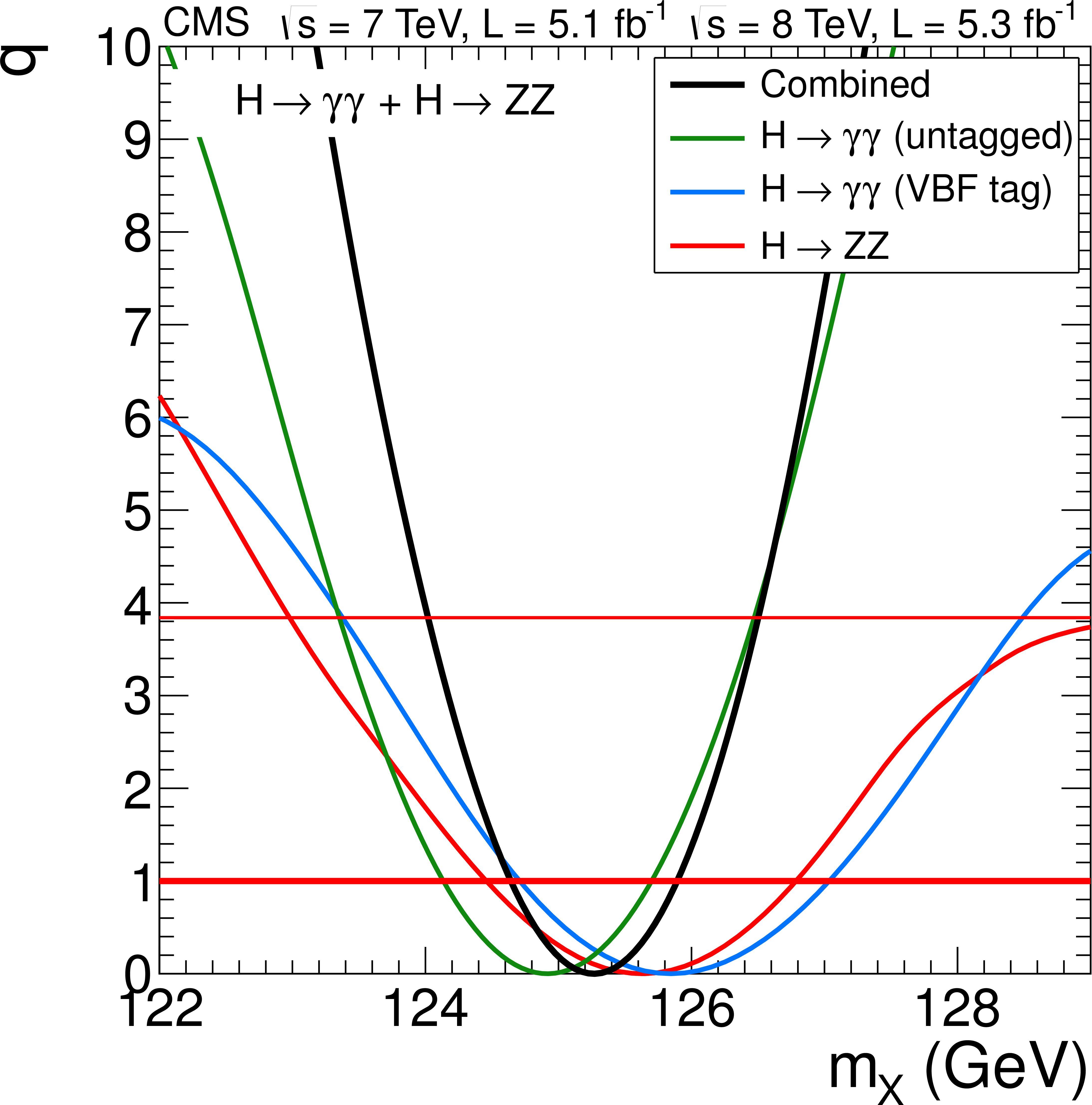
(Left) The 2D 68% CL contours for a hypothesized boson mass $m_{X}$ versus $\mu = \sigma / \sigma _{\mathrm {SM}}$ for the untagged $\gamma \gamma $, VBF-tagged $\gamma \gamma $, and $ {\mathrm {Z}} {\mathrm {Z}}\to 4\ell $ decay channels, and their combination from the combined 7 and 8 TeV data. In the combination, the relative signal strengths for the three final states are fixed to those for the SM Higgs boson. (Right) The maximum-likelihood test statistic $q$ versus $m_{\mathrm {X}}$ for the untagged $\gamma \gamma $, VBF-tagged $\gamma \gamma $, and $ {\mathrm {Z}} {\mathrm {Z}}\to 4\ell $ final states, and their combination from the combined 7 and 8 TeV data. Neither the absolute nor the relative signal strengths for the three final states are constrained to the SM Higgs boson expectations. The crossings with the thick (thin) horizontal line $q=1$ define the 68% (95%) CL interval for the measured mass, shown by the vertical lines. |
png pdf |
Figure 38-b:
(Left) The 2D 68% CL contours for a hypothesized boson mass $m_{X}$ versus $\mu = \sigma / \sigma _{\mathrm {SM}}$ for the untagged $\gamma \gamma $, VBF-tagged $\gamma \gamma $, and $ {\mathrm {Z}} {\mathrm {Z}}\to 4\ell $ decay channels, and their combination from the combined 7 and 8 TeV data. In the combination, the relative signal strengths for the three final states are fixed to those for the SM Higgs boson. (Right) The maximum-likelihood test statistic $q$ versus $m_{\mathrm {X}}$ for the untagged $\gamma \gamma $, VBF-tagged $\gamma \gamma $, and $ {\mathrm {Z}} {\mathrm {Z}}\to 4\ell $ final states, and their combination from the combined 7 and 8 TeV data. Neither the absolute nor the relative signal strengths for the three final states are constrained to the SM Higgs boson expectations. The crossings with the thick (thin) horizontal line $q=1$ define the 68% (95%) CL interval for the measured mass, shown by the vertical lines. |
png pdf |
Figure 39:
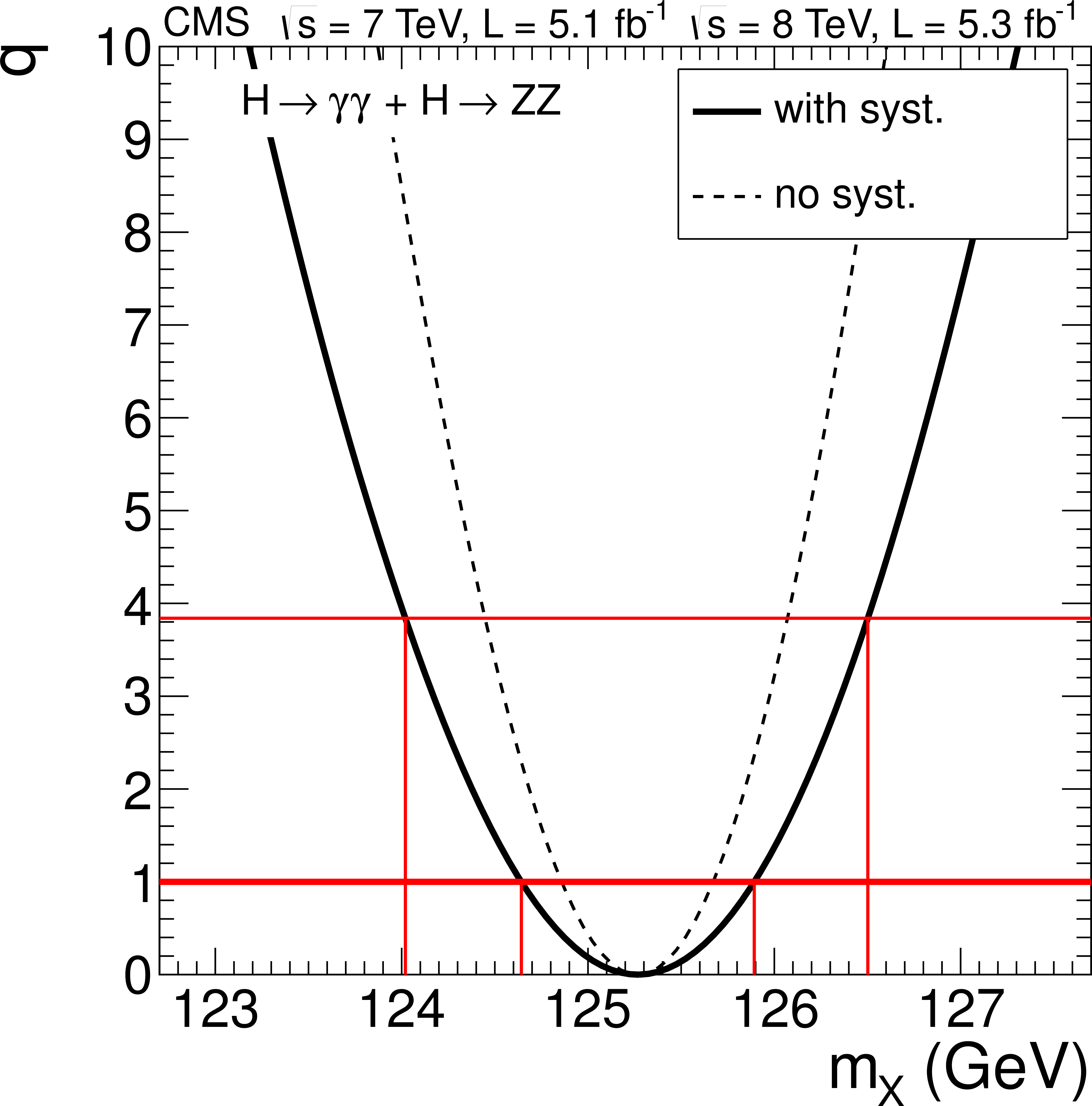
The maximum-likelihood test statistic $q$ versus the hypothesized boson mass $m_{\mathrm {X}}$ for the combination of the $\gamma \gamma $ and $ {\mathrm {Z}} {\mathrm {Z}}\to 4\ell $ modes from the combined 7 and 8 TeV data. The solid line is obtained including all the nuisance parameters and, hence, includes both the statistical and systematic uncertainties. The dashed line is found with all nuisance parameters fixed to their best-fit values and, hence, represents the statistical uncertainties only. The crossings with the thick (thin) horizontal line $q=1$ (3.8) define the 68% (95%) CL interval for the measured mass, shown by the vertical lines. |
png pdf |
Figure 40:
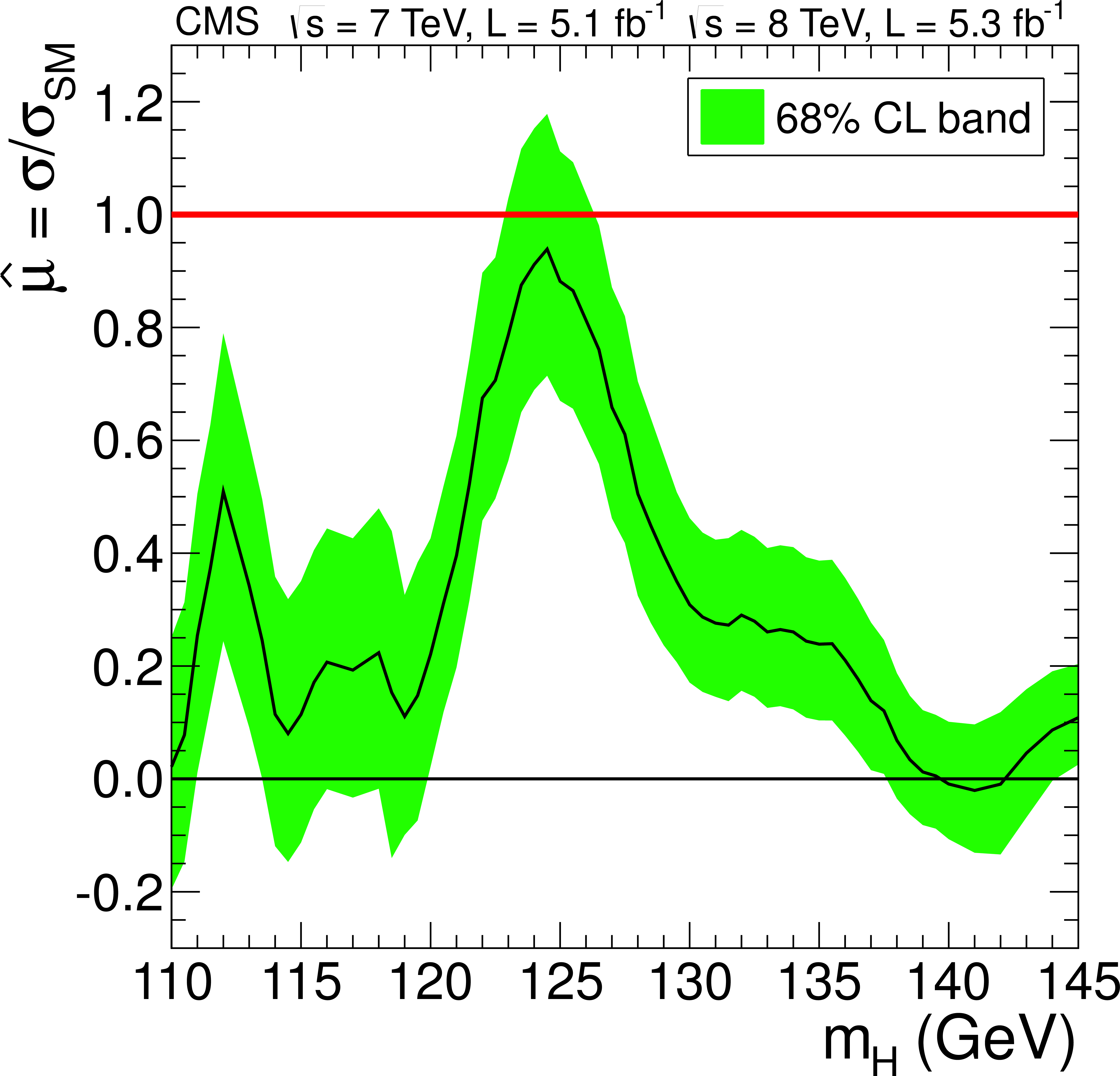
The signal-strength $\hat{\mu} = \sigma / \sigma _\mathrm {SM}$ as a function of the hypothesized SM Higgs boson mass $ {m_{ {\mathrm {H}} }}$ using all the decay modes and the combined 7 and 8 TeV data sets. The bands correspond to ${\pm }1$ standard deviation including both statistical and systematic uncertainties. |
png pdf |
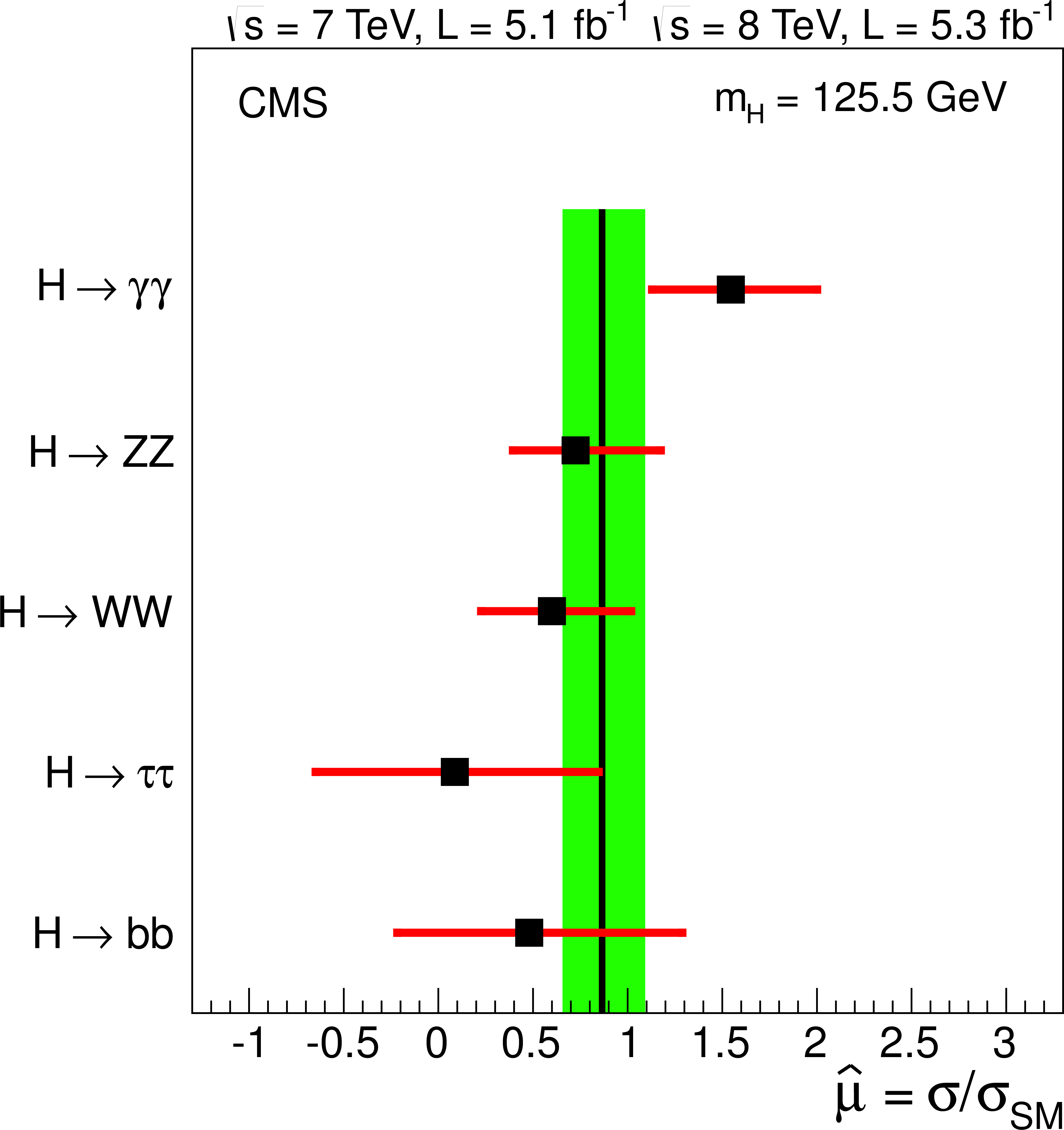
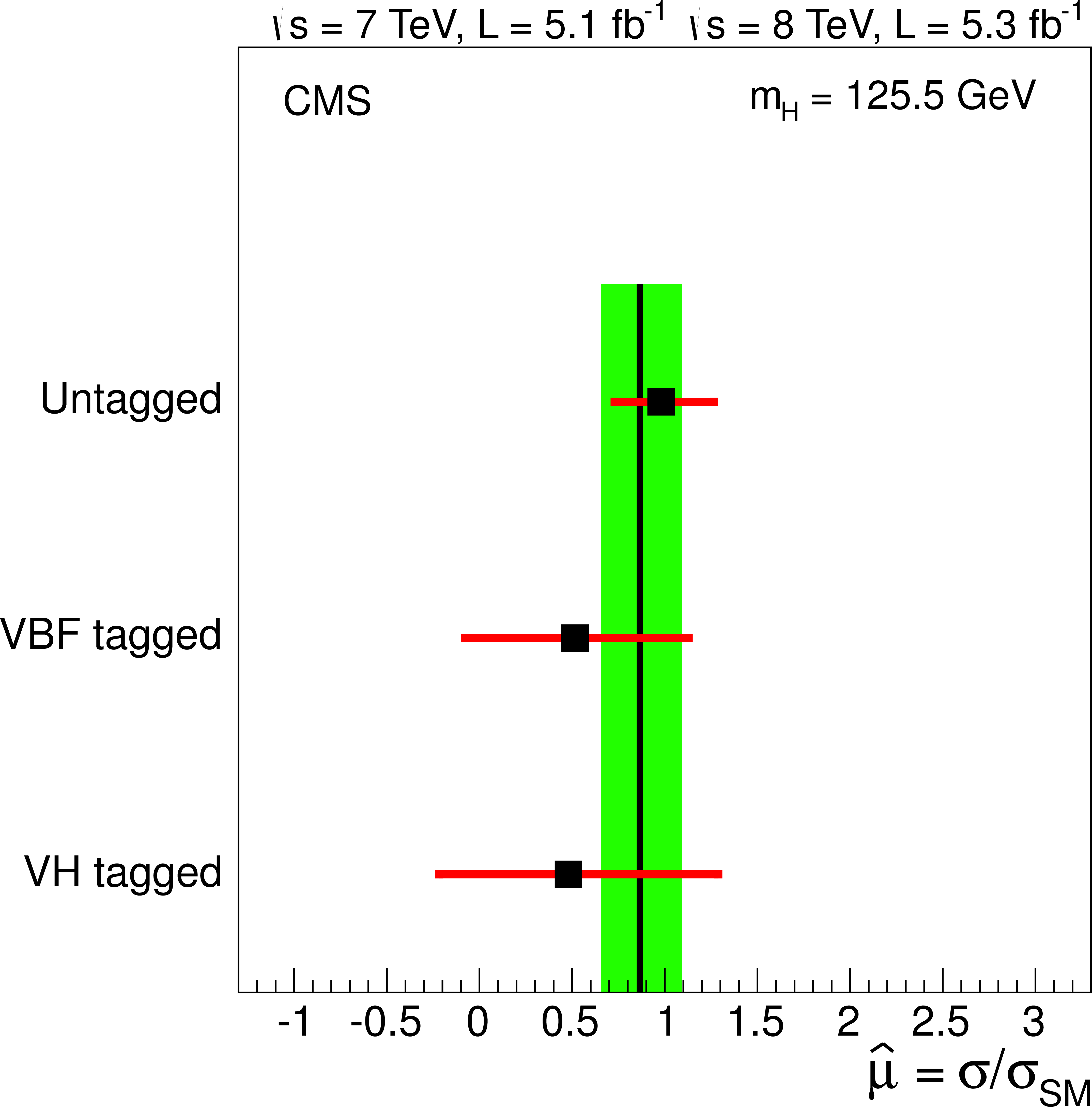
Figure 41-a:
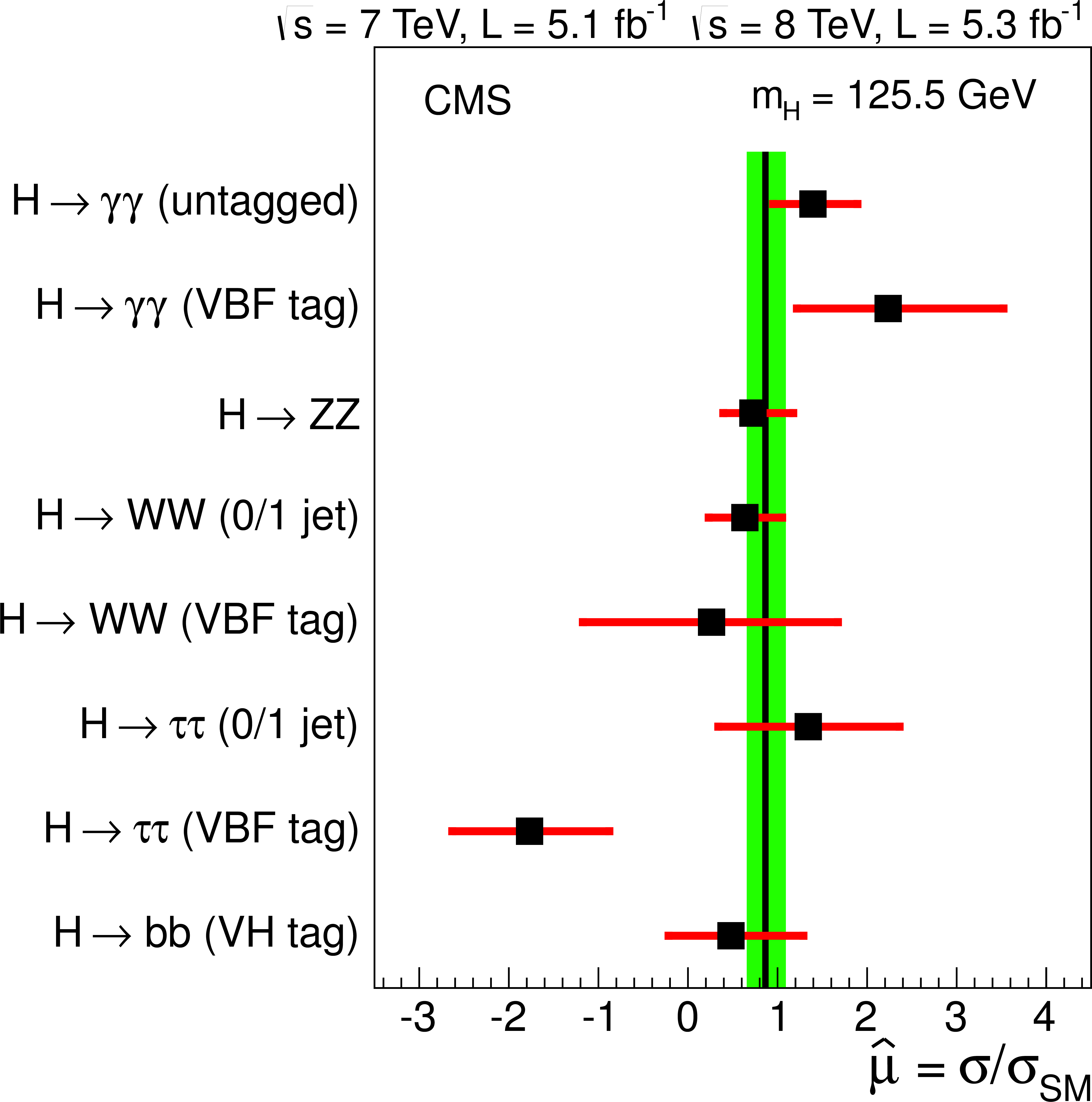
Signal-strength values $\hat{\mu} = \sigma / \sigma _\mathrm {SM}$ for various combinations of the search channels with $ {m_{ {\mathrm {H}} }}=125.5 GeV $. The horizontal bars indicate the $\pm 1 \sigma $ statistical-plus-systematic uncertainties. The vertical line with the band shows the combined $\hat{\mu} $ value with its uncertainty. (Top) Combinations by decay mode and additional requirements that select events with an enriched purity of a particular production mechanism. (Bottom-left) Combinations by decay mode. (Bottom-right) Combinations by selecting events with additional requirements that select events with an enriched purity of a particular production mechanism. |
png pdf |
Figure 41-b:
Signal-strength values $\hat{\mu} = \sigma / \sigma _\mathrm {SM}$ for various combinations of the search channels with $ {m_{ {\mathrm {H}} }}=125.5 GeV $. The horizontal bars indicate the $\pm 1 \sigma $ statistical-plus-systematic uncertainties. The vertical line with the band shows the combined $\hat{\mu} $ value with its uncertainty. (Top) Combinations by decay mode and additional requirements that select events with an enriched purity of a particular production mechanism. (Bottom-left) Combinations by decay mode. (Bottom-right) Combinations by selecting events with additional requirements that select events with an enriched purity of a particular production mechanism. |
png pdf |
Figure 41-c:
Signal-strength values $\hat{\mu} = \sigma / \sigma _\mathrm {SM}$ for various combinations of the search channels with $ {m_{ {\mathrm {H}} }}=125.5 GeV $. The horizontal bars indicate the $\pm 1 \sigma $ statistical-plus-systematic uncertainties. The vertical line with the band shows the combined $\hat{\mu} $ value with its uncertainty. (Top) Combinations by decay mode and additional requirements that select events with an enriched purity of a particular production mechanism. (Bottom-left) Combinations by decay mode. (Bottom-right) Combinations by selecting events with additional requirements that select events with an enriched purity of a particular production mechanism. |
png pdf |
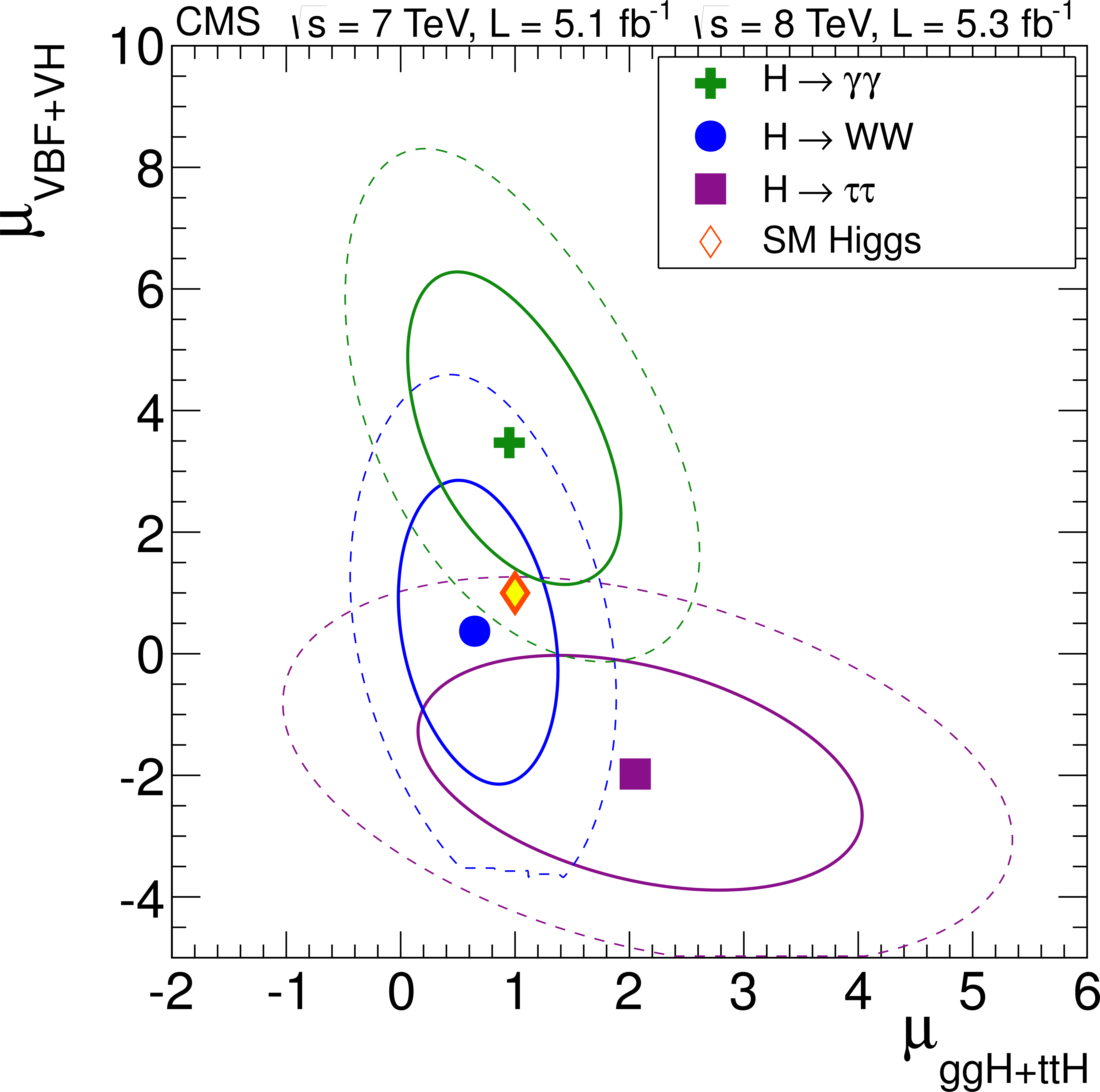
Figure 42:
The 68% (solid lines) and 95% (dashed lines) CL contours for the signal strength of the gluon-gluon fusion plus $ {\mathrm {t}} {\mathrm {t}} {\mathrm {H}} $ production mechanisms ($\mu _{ {\mathrm {g}} {\mathrm {g}} {\mathrm {H}} + {\mathrm {t}} {\mathrm {t}} {\mathrm {H}} }$), versus VBF plus VH ($\mu _{\mathrm {VBF+VH}}$). The three different lines show the results for the decay modes: $\gamma \gamma $, $ {\mathrm {W}} {\mathrm {W}}$, and $\tau \tau $. The markers indicate the best-fit values for each mode. The diamond at (1,1) indicates the expected values for the SM Higgs boson. |
png pdf |
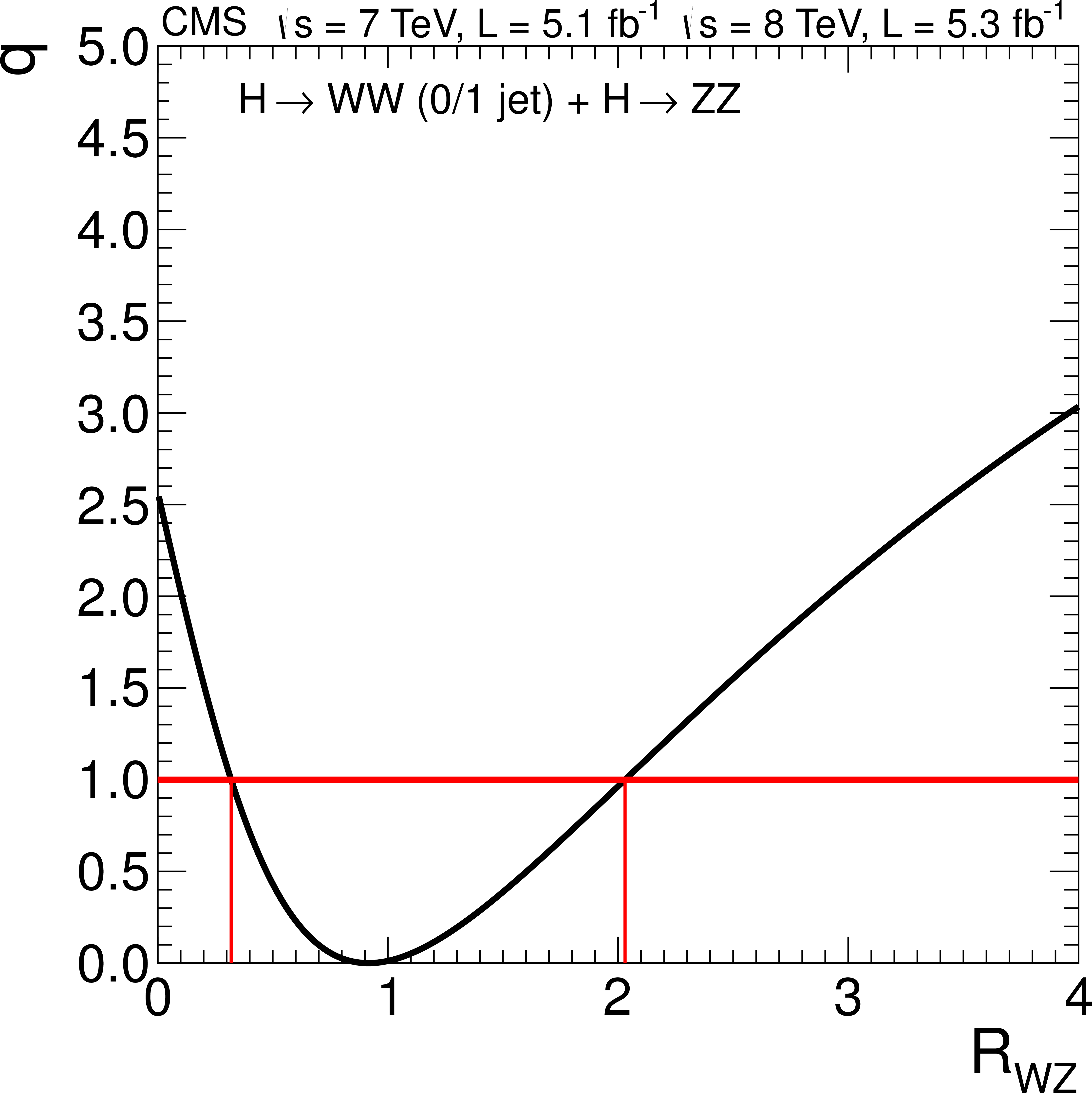
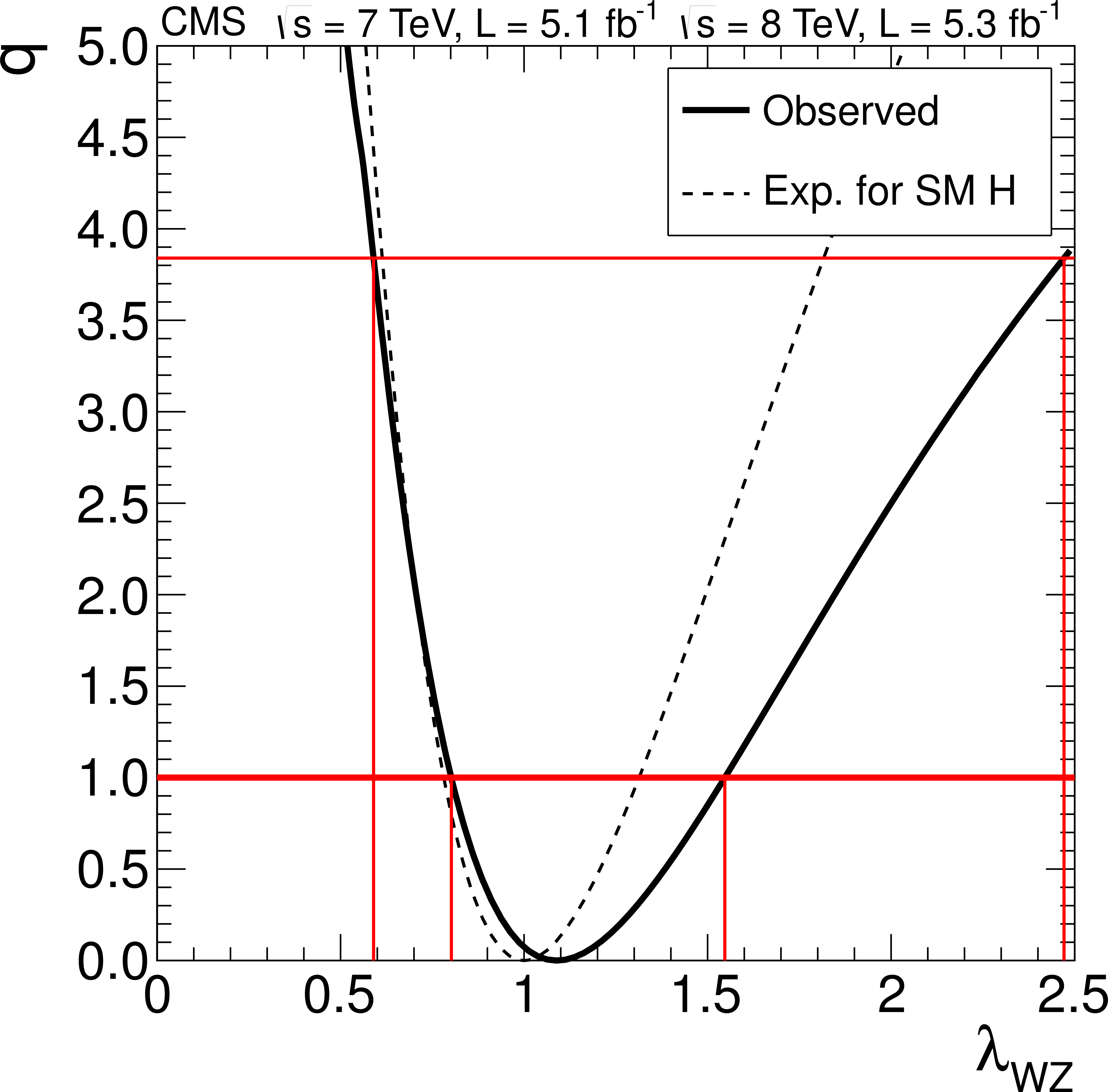
Figure 43-a:
(Left) The likelihood test statistic $q(R_{ {\mathrm {W}} {\mathrm {Z}}})$ as a function of the event-rate modifier $R_{ {\mathrm {W}} {\mathrm {Z}}}$ from the combined untagged $ {\mathrm {H}} \to {\mathrm {W}} {\mathrm {W}}\to \ell {\nu }\ell {\nu }$ and inclusive $ {\mathrm {H}} \to {\mathrm {Z}} {\mathrm {Z}}\to 4\ell $ searches. (Right) The test statistic $q(\lambda _{ {\mathrm {W}} {\mathrm {Z}}})$ as a function of the ratio of the couplings to $ {\mathrm {W}}$ and $ {\mathrm {Z}}$ bosons, $\lambda _{ {\mathrm {W}} {\mathrm {Z}}}$, from the combination of all channels. The intersection of the curves with the horizontal lines $q= 1$ and 3.8 give the 68% and 95% CL intervals, respectively. |
png pdf |
Figure 43-b:
(Left) The likelihood test statistic $q(R_{ {\mathrm {W}} {\mathrm {Z}}})$ as a function of the event-rate modifier $R_{ {\mathrm {W}} {\mathrm {Z}}}$ from the combined untagged $ {\mathrm {H}} \to {\mathrm {W}} {\mathrm {W}}\to \ell {\nu }\ell {\nu }$ and inclusive $ {\mathrm {H}} \to {\mathrm {Z}} {\mathrm {Z}}\to 4\ell $ searches. (Right) The test statistic $q(\lambda _{ {\mathrm {W}} {\mathrm {Z}}})$ as a function of the ratio of the couplings to $ {\mathrm {W}}$ and $ {\mathrm {Z}}$ bosons, $\lambda _{ {\mathrm {W}} {\mathrm {Z}}}$, from the combination of all channels. The intersection of the curves with the horizontal lines $q= 1$ and 3.8 give the 68% and 95% CL intervals, respectively. |
png pdf |
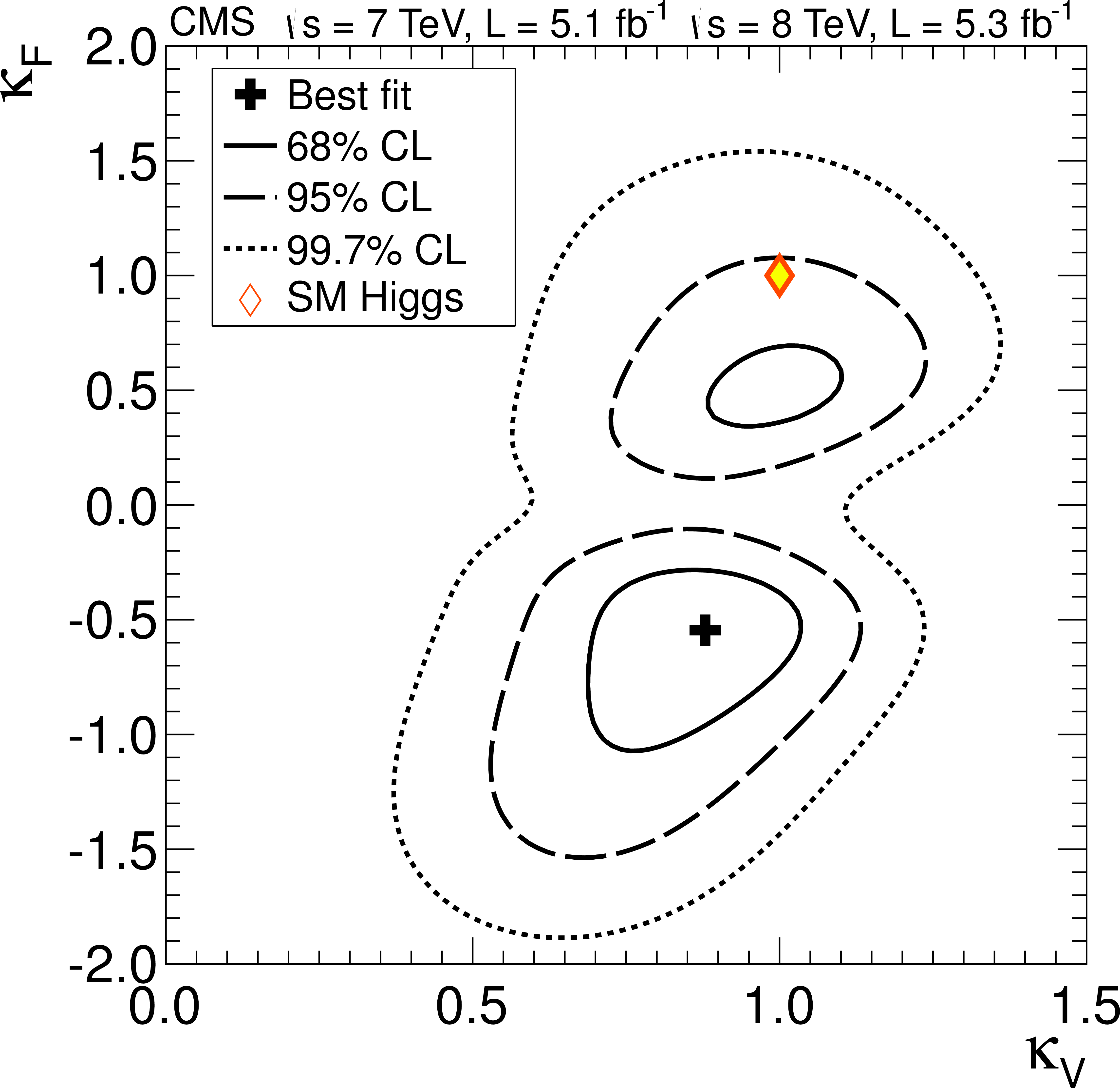
Figure 44-a:
The likelihood test statistic in the $\kappa _V$ versus $\kappa _F$ plane. The cross indicates the best-fit values. The solid, dashed, and dotted lines show the 68%, 95%, and 99.7% CL contours, respectively. The diamond shows the SM point $(\kappa _V, \kappa _F)$ = (1, 1). The left plot allows for different signs of $\kappa _V$ and $\kappa _F$, while the right plot constrains them both to be positive. |
png pdf |
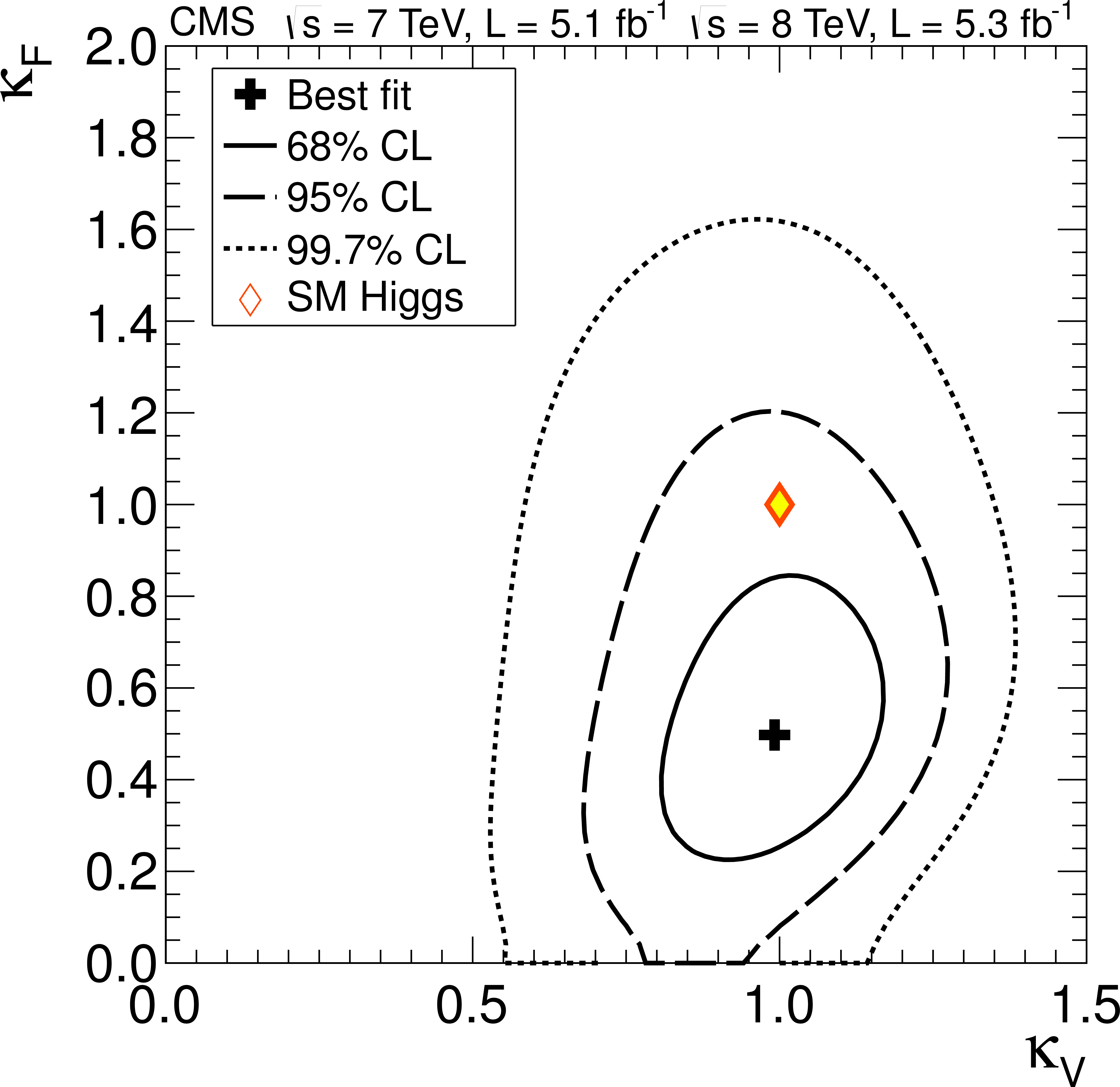
Figure 44-b:
The likelihood test statistic in the $\kappa _V$ versus $\kappa _F$ plane. The cross indicates the best-fit values. The solid, dashed, and dotted lines show the 68%, 95%, and 99.7% CL contours, respectively. The diamond shows the SM point $(\kappa _V, \kappa _F)$ = (1, 1). The left plot allows for different signs of $\kappa _V$ and $\kappa _F$, while the right plot constrains them both to be positive. |

png pdf |
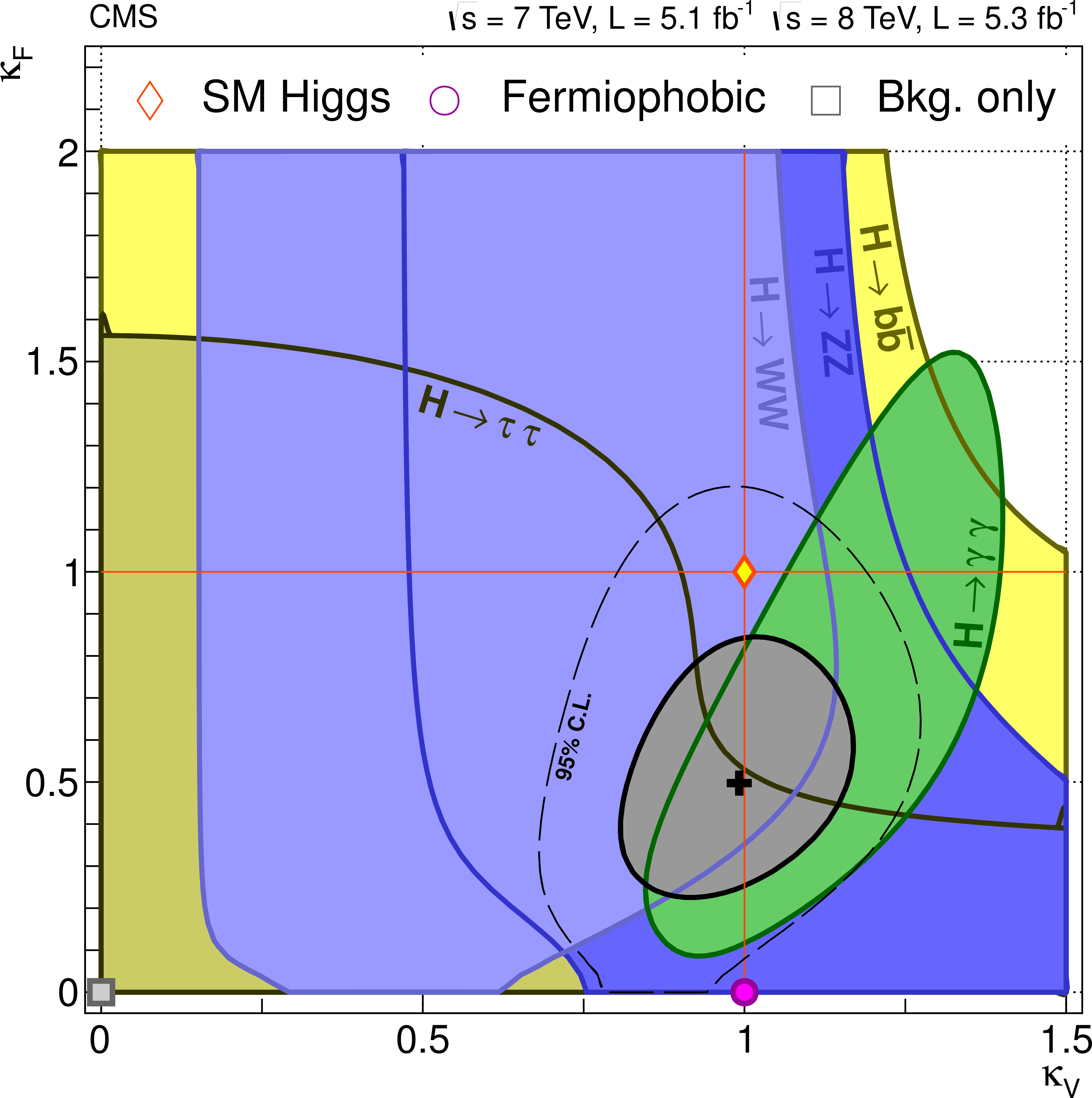
Figure 45-a:
The 68% CL contours for the test statistic in the $(\kappa _V$ versus $\kappa _F)$ plane for individual channels (coloured regions) and the overall combination (solid thick lines). The thin dashed lines show the 95% CL range for the overall combination. The black cross indicates the global best-fit values. The diamond shows the SM Higgs boson point $(\kappa _V, \kappa _F)$ = (1, 1). The point $(\kappa _V, \kappa _F)$ = (1, 0), indicated by the circle, corresponds to the fermiophobic Higgs boson scenario. The left plot allows for different signs of $\kappa _V$ and $\kappa _F$, while the right plot constrains them both to be positive. |
png pdf |
Figure 45-b:
The 68% CL contours for the test statistic in the $(\kappa _V$ versus $\kappa _F)$ plane for individual channels (coloured regions) and the overall combination (solid thick lines). The thin dashed lines show the 95% CL range for the overall combination. The black cross indicates the global best-fit values. The diamond shows the SM Higgs boson point $(\kappa _V, \kappa _F)$ = (1, 1). The point $(\kappa _V, \kappa _F)$ = (1, 0), indicated by the circle, corresponds to the fermiophobic Higgs boson scenario. The left plot allows for different signs of $\kappa _V$ and $\kappa _F$, while the right plot constrains them both to be positive. |
png pdf |
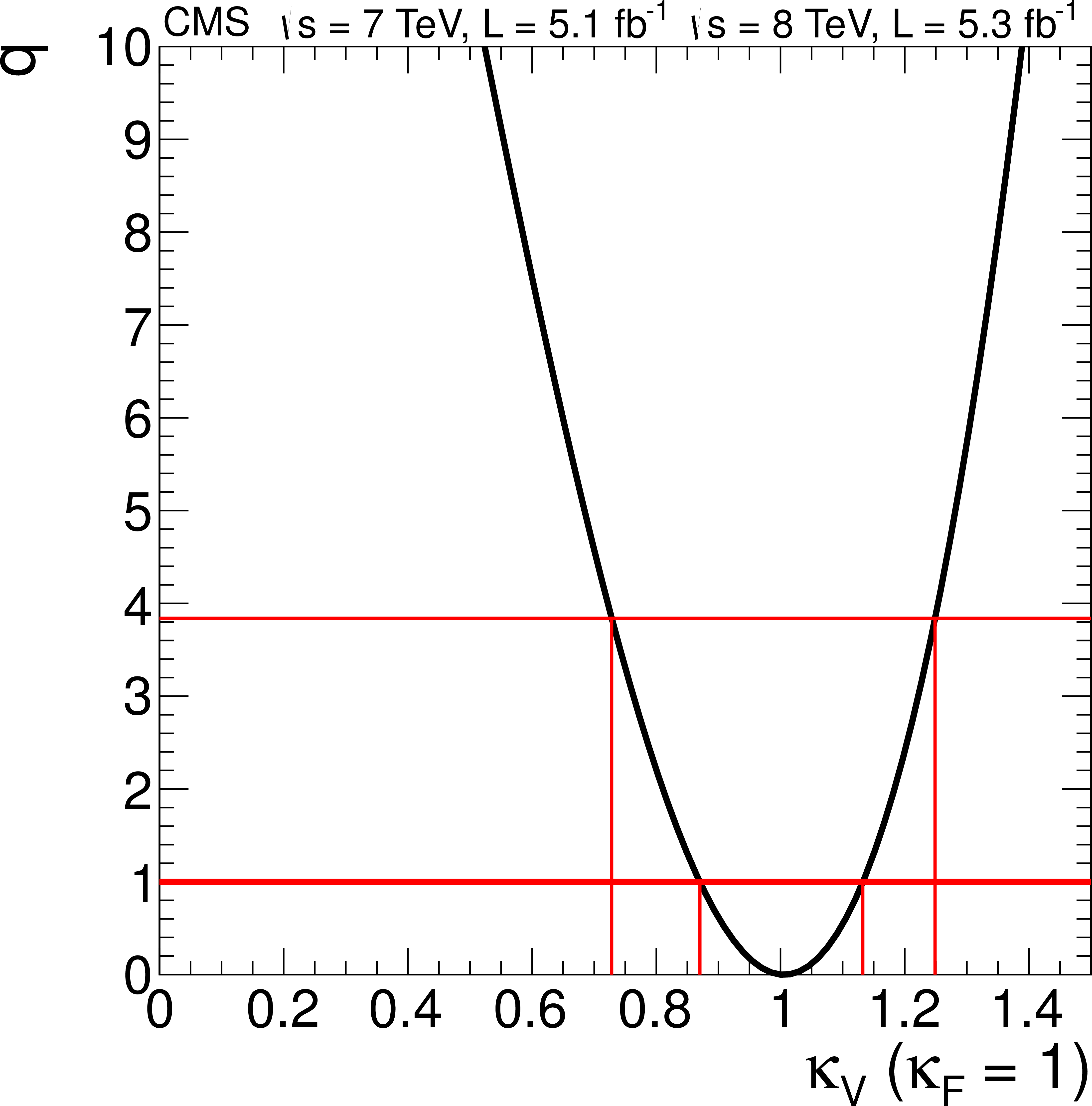
Figure 46-a:
The likelihood test statistic $q(\kappa _V;\kappa _F=1)$ (left) and $q(\kappa _F;\kappa _V=1)$ (right). The intersections with the horizontal lines $q=1$ and $q=3.84$ mark the 68% and 95% CL intervals, respectively, as shown by the vertical lines. |
png pdf |
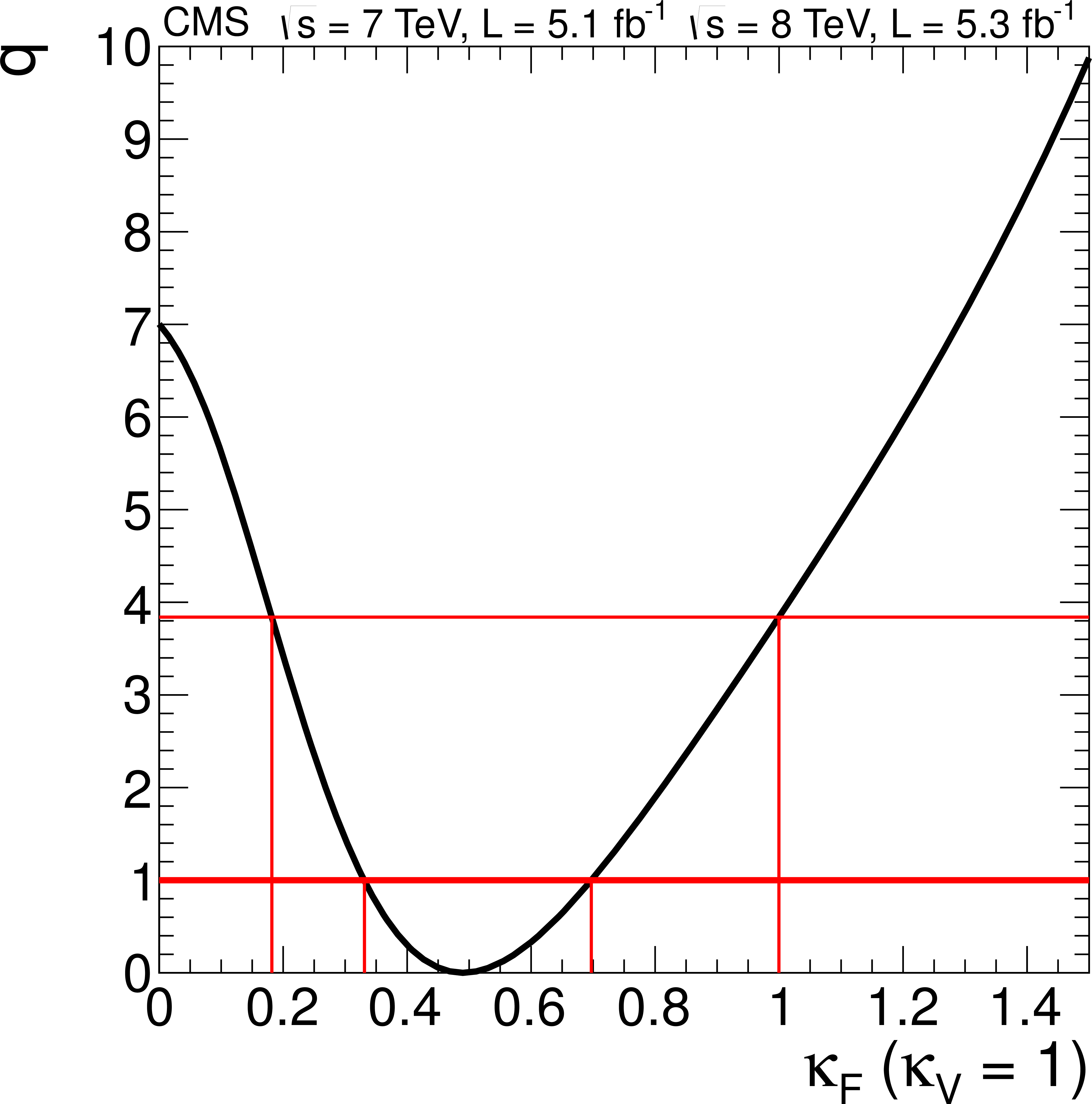
Figure 46-b:
The likelihood test statistic $q(\kappa _V;\kappa _F=1)$ (left) and $q(\kappa _F;\kappa _V=1)$ (right). The intersections with the horizontal lines $q=1$ and $q=3.84$ mark the 68% and 95% CL intervals, respectively, as shown by the vertical lines. |
png pdf |
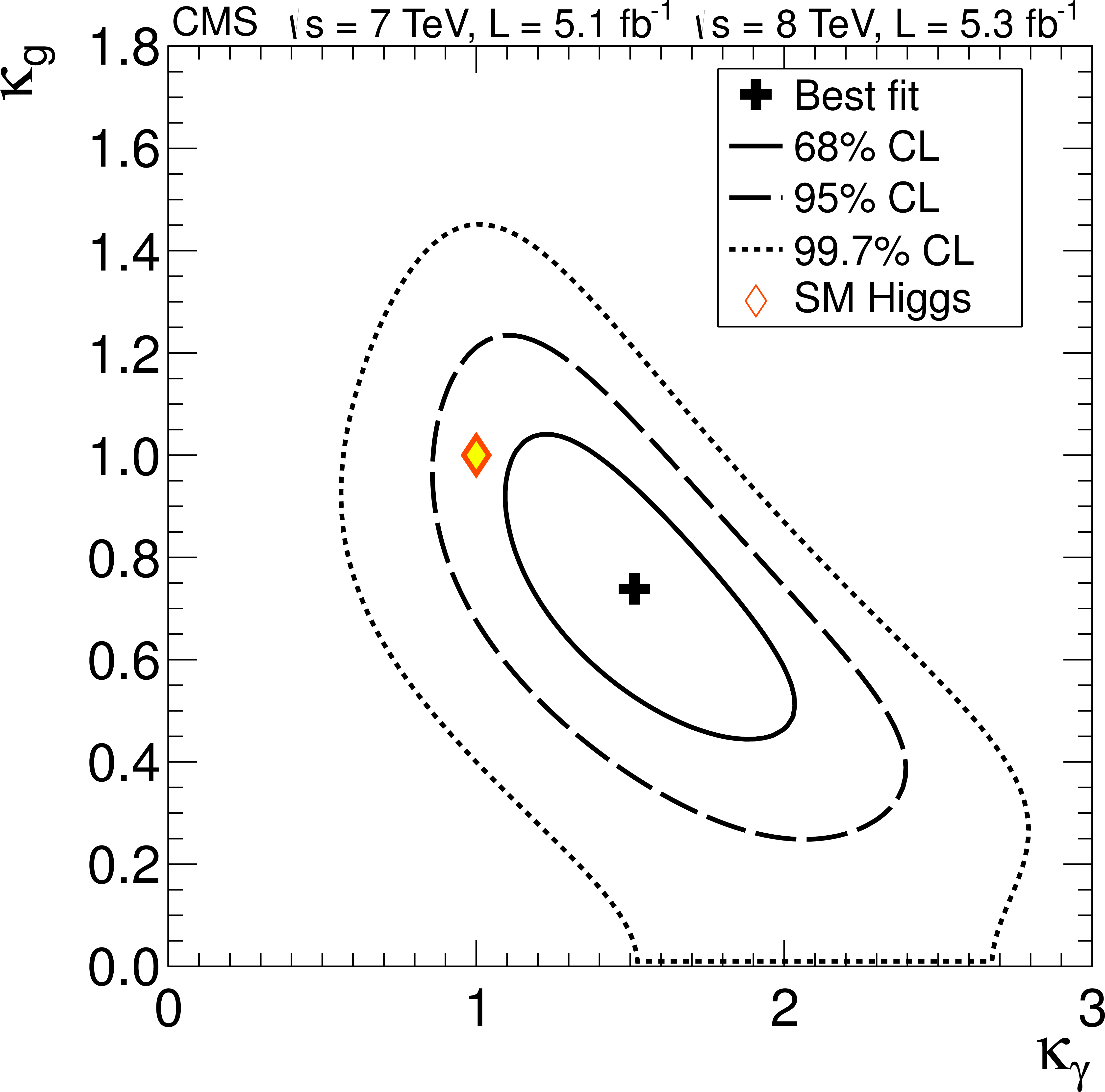
Figure 47:
The likelihood test statistic $q(\kappa _{ {\gamma }}, \kappa _ {\mathrm {g}})$ assuming $\Gamma _{\mathrm {BSM}}=0$. The cross indicates the best-fit values. The solid, dashed, and dotted contours show the 68%, 95%, and 99.7% CL contours, respectively. The diamond shows the SM point $(\kappa _{ {\gamma }}, \kappa _ {\mathrm {g}})$ = (1, 1). The partial widths associated with the tree-level production processes and decay modes are assumed to be unaltered ($\kappa = 1$). |
png pdf |
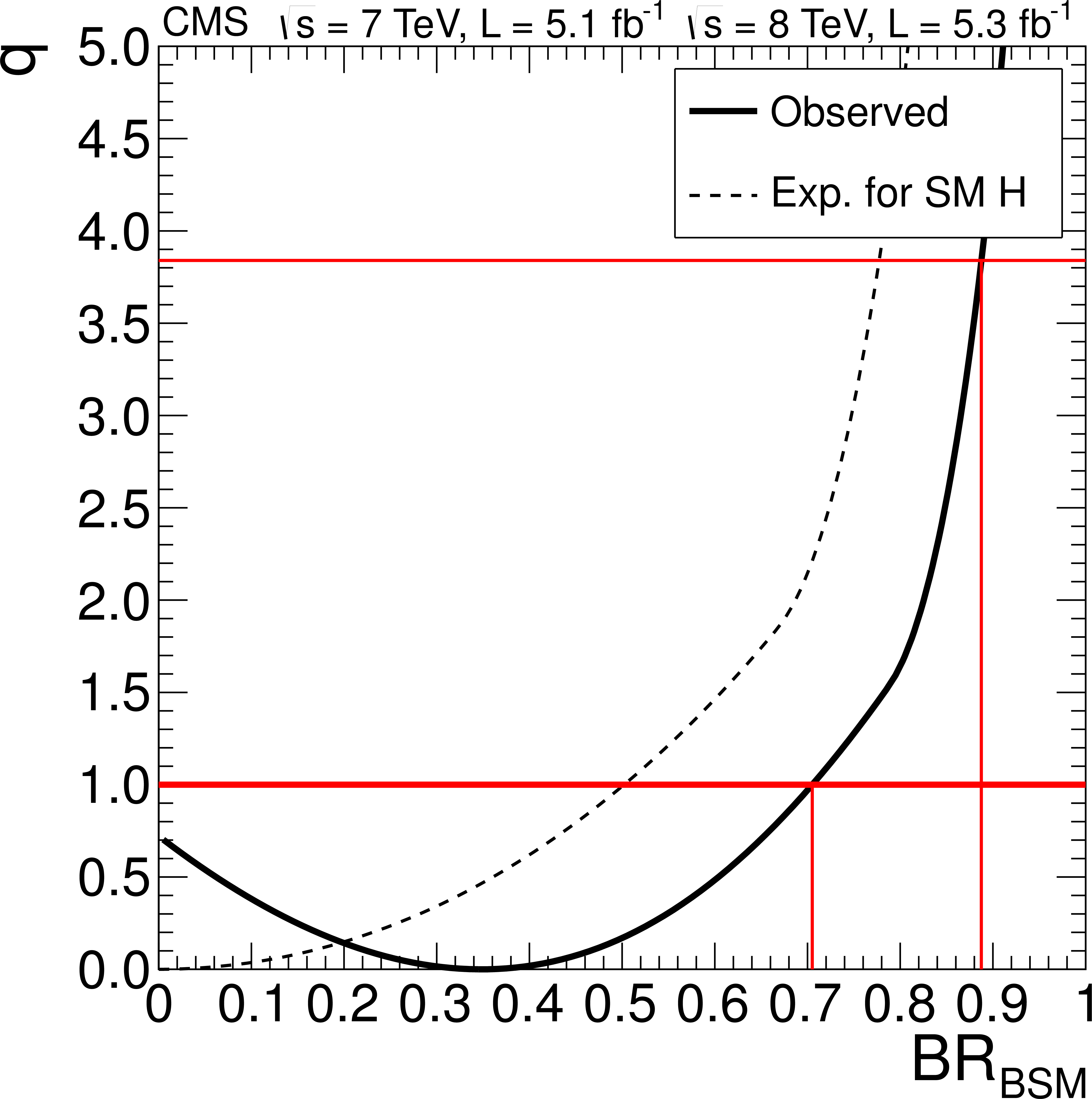
Figure 48:
The likelihood test statistic $q$ versus $\mathrm {BR}_{\mathrm {BSM}}=\Gamma _{\mathrm {BSM}}/\Gamma _{\mathrm {tot}}$, with the parameters $\kappa _ {\mathrm {g}}$ and $\kappa _{ {\gamma }}$ included as nuisance parameters. The solid curve is the data; the dashed curve indicates the expected median results in the presence of the SM Higgs boson. The intersections with the horizontal lines $q=$ 1 and 3.8 give the 68% and 95% CL intervals, respectively. The partial widths associated with the tree-level production processes and decay modes are assumed to be unaltered ($\kappa = 1$). |
png pdf |
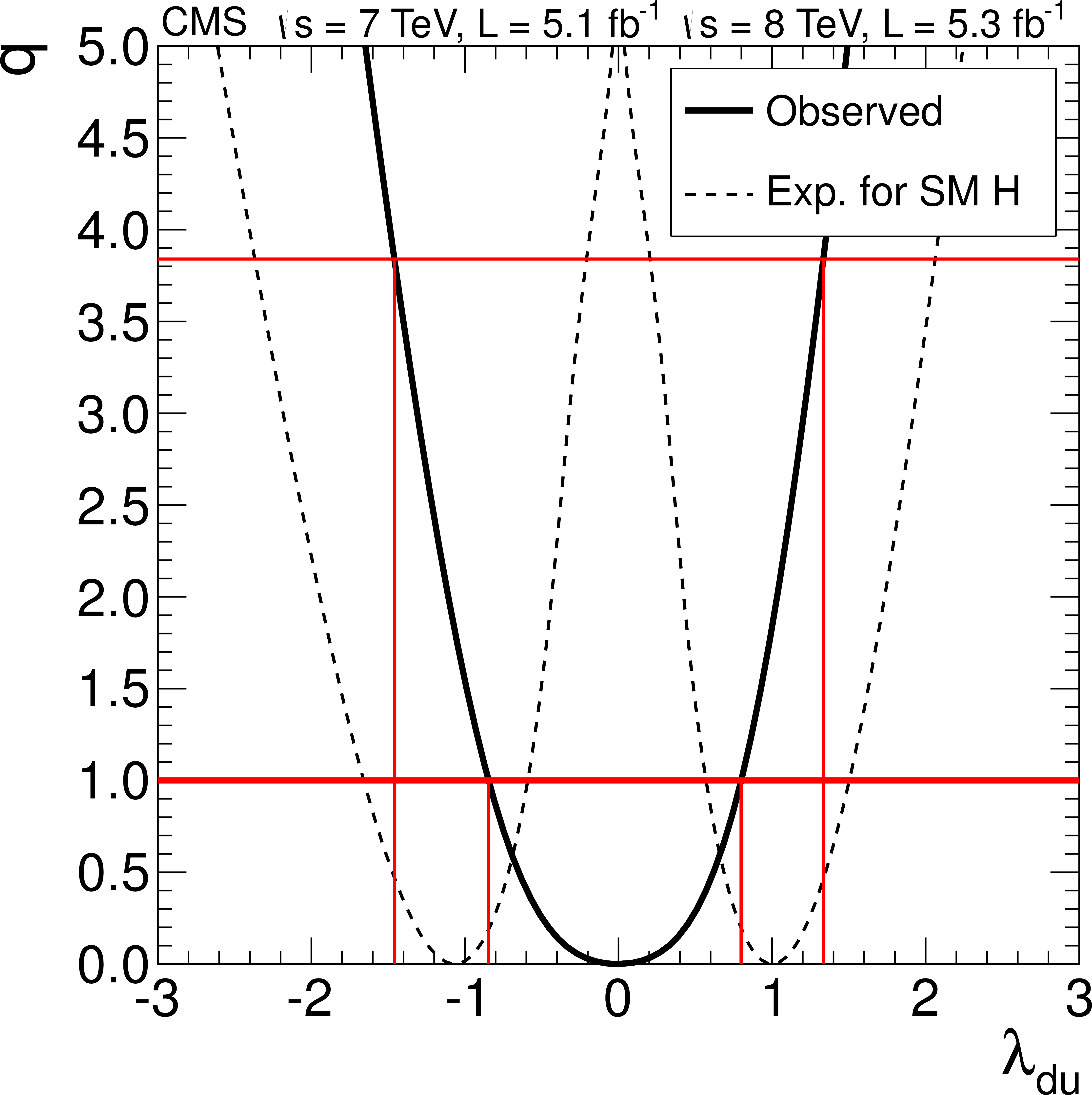
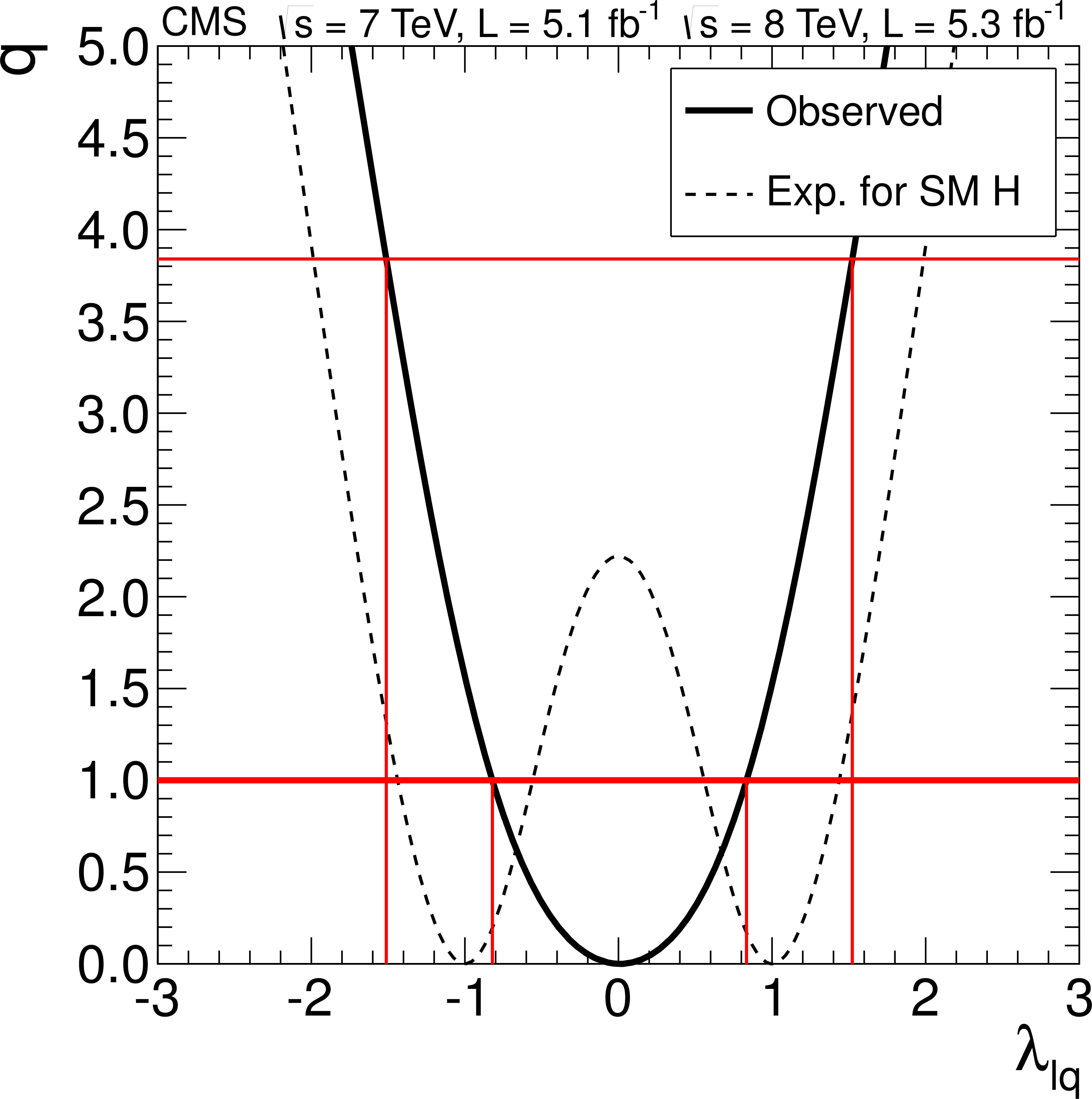
Figure 49-a:
(Left) Likelihood test statistic $q$ as a function of the ratio $\lambda _{\mathrm {du}}$ of the coupling to the up- and down-type fermions with the coupling modifiers $\kappa _V$ and $\kappa _{\mathrm {u}}$ treated as nuisance parameters. (Right) The likelihood test statistic as a function of the ratio $\lambda _{\ell \mathrm {q}}$ of the couplings to leptons and quarks with the coupling modifiers $\kappa _V$ and $\kappa _{\mathrm {q}}$ treated as nuisance parameters. The solid curves are the results from the data. The dashed curves show the expected distributions for the SM Higgs boson. The intersection of the curves with the horizontal lines $q=$1 and 3.8 give the 68% and 95% CL intervals, respectively. |
png pdf |
Figure 49-b:
(Left) Likelihood test statistic $q$ as a function of the ratio $\lambda _{\mathrm {du}}$ of the coupling to the up- and down-type fermions with the coupling modifiers $\kappa _V$ and $\kappa _{\mathrm {u}}$ treated as nuisance parameters. (Right) The likelihood test statistic as a function of the ratio $\lambda _{\ell \mathrm {q}}$ of the couplings to leptons and quarks with the coupling modifiers $\kappa _V$ and $\kappa _{\mathrm {q}}$ treated as nuisance parameters. The solid curves are the results from the data. The dashed curves show the expected distributions for the SM Higgs boson. The intersection of the curves with the horizontal lines $q=$1 and 3.8 give the 68% and 95% CL intervals, respectively. |
|
|
Compact Muon Solenoid LHC, CERN |
|

|

|

|

|

|