This website is no longer maintained. Its content may be obsolete. Please visit http://home.cern/ for current CERN information.
Thorsten Ohl (TH Darmstadt, Theoretical High Energy Physics Group)
e-mail: Thorsten.Ohl@Physik.TH-Darmstadt.de
This is the second article in a series describing the LaTeX
package FeynMF for easy drawing of professional quality Feynman
diagrams with METAFONT (or MetaPost). This time more
advanced topics are covered.
Here are links to the
First
and
Third
article in the series.
In [1], I have described the design principles and simple applications of FeynMF [2]. Now it is time to discuss the more esoteric features of FeynMF that allow efficient creation of rather complicated Feynman diagrams. In this article the emphasis will be on the so called immediate mode, while the extension mechanism will be discussed in the third and final article.
Most computer graphics systems offer two modes, commonly called display list mode and immediate mode. The latter performs the drawing operations immediately (whence the name), while the former compiles them into a display list which is executed later.
In addition to the graph mode discussed earlier, which corresponds to display list mode, FeynMF offers an immediate mode in which drawing operations are performed immediately. There is another distinction that should be kept in mind: graph mode operates on abstract vertices and how they are connected, while immediate mode works directly with the coordinates of vertices and the arcs (called paths in [3]) connecting them.
With minor exceptions, FeynMF's graph mode will produce straight lines only. Therefore one of immediate mode's most important applications is the drawing of diagrams with unusually curved arcs. These curved arcs can be drawn in the same line styles as the arcs in graph mode. This feature allows us to combine the two modes for maximizing the expressive power and convenience of FeynMF.
A comprehensive discussion of METAFONT's facilities for constructing curves is far beyond the scope of this tutorial. Interested readers should consult the first chapters of [3] for the definitive guide.
FeynMF's immediate mode commands are easily recognized by their \fmfi prefix. They are listed in [2,4]. The most important command is \fmfi, which is similar to \fmf, except that the second argument is no longer a set of vertices, but a METAFONT expression expanding to a path on which the arc will be drawn in the style specified in the first argument. Similarly, \fmfiv behaves like \fmfv but takes the coordinates of a vertex as second argument.
\fmfforce is used to import immediate mode coordinates to graph
mode, while vpath and vloc are used to import graph mode
coordinates to immediate mode. Examples are given below and readers
should consult [2,4] for a formal description.
METAFONT constructs paths by connecting vertices with Bezier curves
(see [3] for details). The basic operator for connecting
vertices smoothly is ``..''. The following example defines a
generic macro for the examples below and demonstrates the use of the
``..'' operator''
\gdef\P#1#2{%
\begin{fmfgraph*}(35,15)
\fmfi{#1}{#2}
\def\L##1##2{\fmfiv{%
dec.shape=circle,dec.size=3thin,
dec.fill=1,lab.dist=5thick,
lab=\noexpand\texttt{%
\noexpand\scriptsize ##1}}{##2}}
\L{sw}{sw}\L{.3[nw,,ne]}{.3[nw,ne]}
\L{ne}{ne}\L{.7[sw,,se]}{.7[sw,se]}
\end{fmfgraph*}}
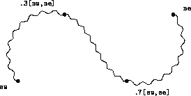
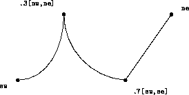
\P{plain}{sw .. .3[nw,ne]
.. .7[sw,se] .. ne}
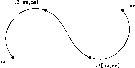
The bracket construct .3[nw,ne] should be read ``the point
30% of the way from nw to ne'' and is equivalent to
0.7 nw + 0.3 ne.
Besides predefining the corners as nw, sw,
se and ne,
FeynMF's \fmfi adds to METAFONT's draw the ability to draw
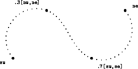
the paths in various styles, such as dotted
\P{dots}{sw .. .3[nw,ne]
  .. .7[sw,se] .. ne}
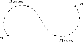
dashed:
\P{dashes}{sw .. .3[nw,ne]
  .. .7[sw,se] .. ne}
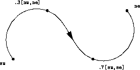
or with an arrow:
\P{fermion}{sw .. .3[nw,ne]
  .. .7[sw,se] .. ne}
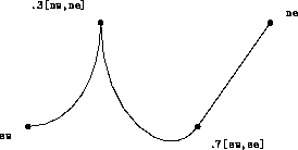
It is also possible to draw wiggly:
\P{photon}{sw .. .3[nw,ne]
  .. .7[sw,se] .. ne}
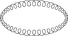
or even curly:
\P{gluon}{sw .. .3[nw,ne]
  .. .7[sw,se] .. ne}
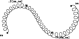
lines along arbitrary paths.
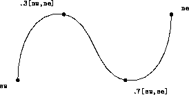
By placing a direction in curly braces next to a vertex, we can fix the direction in which the path will enter or leave this vertex:
\P{plain}{sw{up} .. .3[nw,ne]
  .. .7[sw,se] .. {up}ne}
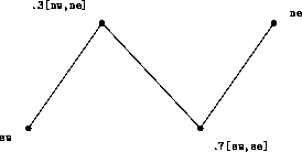
It is also possible to connect vertices with straight lines using the
``--'' operator:
\P{plain}{sw -- .3[nw,ne]
  -- .7[sw,se] -- ne}
These possibilities can be mixed in the same path:
\P{plain}{sw{right} .. {up}.3[nw,ne]{down}
  .. .7[sw,se] -- ne}
This example shows that a straight line will not be connected smoothly
with a neighbouring smooth line. For such a smooth continuation, the
``---'' operator is provided:
\P{plain}{sw{right} .. {up}.3[nw,ne]{down}
  .. .7[sw,se] --- ne}
Circles (possibly scaled) are also readily available:
\begin{fmfgraph}(35,15)
  \fmfi{gluon}{fullcircle
    xscaled w yscaled h shifted c}
\end{fmfgraph}
While this list of examples should be sufficient for all practical purposes, it does not exhaust all the possibilities for constructing paths in METAFONT. A comprehensive account for the curious is given in [3]
Having explained the basic building blocks, I will now continue with realistic applications. I start the examples by describing how to draw two graphs that have been announced in the first part of this tutorial.
 1 \begin{fmfgraph*}(50,60)
 2  \fmfbottom{P1,P2} \fmftop{P1',H',P2'}
 3  \fmf{fermion,tension=2,lab=$P_1$}{P1,g1}
 4  \fmf{fermion,tension=2,lab=$P_2$}{P2,g2}
 5  \fmfblob{.16w}{g1,g2}
 6  \fmf{gluon,lab.side=right,
 7      lab=$x_1P_1$}{g1,v1}
 8  \fmf{gluon,lab.side=right,
 9     lab=$x_2P_2$}{v2,g2}
10  \fmf{fermion,tension=.6}{H,v1,v2,H}
11  \fmfdot{H,v1,v2}
12  \fmf{dbl_dots,lab=$H$}{H,H'}
13  \fmf{fermion}{g1,P1'}
14  \fmf{fermion}{g2,P2'}
15  \fmfv{lab=$g(x_1,,Q^2)$,lab.dist=.1w}{g1}
16  \fmfv{lab=$g(x_2,,Q^2)$,lab.dist=.1w}{g2}
17  \fmffreeze
18  \renewcommand{\P}[3]{\fmfi{plain}{%
19    vpath(__#1,__#2) shifted (thick*(#3))}}
20  \P{P1}{g1}{2,0} \P{P1}{g1}{-2,1}
21  \P{P2}{g2}{2,1} \P{P2}{g2}{-2,0}
22  \P{g1}{P1'}{-2,-1} \P{g1}{P1'}{2,0}
23  \P{g2}{P2'}{-2,0} \P{g2}{P2'}{2,-1}
24 \end{fmfgraph*}
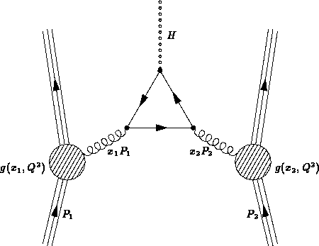
The figure above shows Higgs production through gluon fusion. It is an example of how even complex diagrams can be drawn with very few tuned tension parameters. Since there is no built-in line style for protons, the parallel lines are added ad hoc with the \fmfi command.
In fact this figure repeats the Higgs production diagram from [1] and this time we are in a position to discuss the source code. Lines 1--16 are a straightforward description of the diagram, with some decorations like labels, dots and blobs added. It should need no further comment. Note, however, in lines 15 and 16, that the commas in the TeX labels are doubled, so that FeynMF doesn't interpret them as option separators.
The tension of the lower proton lines (lines 3--4) is increased to make a bit more room in the more crowded top half of the diagram. The tension in the fermion loop is decreased (line 10) to make the loop slightly larger. The latter measure is commonly necessary, because an unweighted least-squared layout will generally produce too small loops.
In line 17 the positions of all vertices are calculated by
\fmffreeze. From then on, we can use the vloc and vpath
function to access the locations of vertices and lines, respectively.
In lines 18 and 19 we use LaTeX's macro facility to define a
shorthand: \Lcs{P{<v_1>}{<v_2>}{<z> will
draw a line parallel to the line connecting v_1 and v_2
shifted by z (the latter measured in units of thick, the
width of thick lines). This macro is used in lines 20--23 to decorate
the external fermion lines, making them look more like compound
states.
Note how the names of vertices are preceded with two underscores
(``__'') in the arguments of vpath. This slight inconvenience in
necessary to separate the namespaces of FeynMF and METAFONT, thereby
avoiding unpleasant surprises if a user accidentally uses a reserved
METAFONT word as a vertex name.
Strictly speaking, lines 18--23 break the concept of structured
markup. This seems appropriate here, because it solves the problem
straightforwardly without needing more advanced METAFONT programming.
Another solution that uses FeynMF's extension mechanism to define a
proton style will be described in the next article.
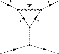
The figures in this section present two very
different ways of drawing so-called ``penguin'' diagrams.
The first (straightforward) figure uses FeynMF graph mode and
reproduces the standard way of drawing these diagrams. As usual the
tension parameter is used to increase the size of the loop compared
to the default.
 1 \begin{fmfgraph*}(35,40)
 2  \fmftop{b,s} \fmfbottom{ep,em}
 3  \fmf{fermion,lab=$b$,lab.sid=left}{b,Vtb}
 4  \fmf{fermion,lab=$s$,lab.sid=left}{Vts,s}
 5  \fmf{fermion,tension=.5,
 6    lab=$t$,lab.sid=right}{Vtb,g,Vts}
 7  \fmf{dbl_wiggly,tension=.5,
 8    lab=$W$,lab.sid=left}{Vtb,Vts}
 9  \fmf{photon}{g,g'}
10  \fmf{fermion}{ep,g',em}
11  \fmfdot{Vtb,Vts,g,g'}
12 \end{fmfgraph*}
But we can also use FeynMF's immediate mode to draw the ``penguin'
diagram in the way it was drawn by John Ellis and Melissa Franklin.
In line 2 the vertices are declared and in lines 3-11 the
\fmfiequ macro is used to establish linear equations among them
(\Lcs{fmfiequ{<expr_1>}{<expr_2>} corresponds to
<expr>_1=<expr_2>; in METAFONT).
 1 \begin{fmfgraph*}(35,40)
 2  \fmfipair{Vtb,Vts,b,s,ep,em,p,p'}
 3  \fmfiequ{.5[Vtb,Vts]}{.5[nw,ne]}
 4  \fmfiequ{Vts}{Vtb+(.3w,0)}
 5  \fmfiequ{b}{.7[sw,nw]}
 6  \fmfiequ{s}{.7[se,ne]}
 7  \fmfiequ{xpart(p')}{xpart(.5[ep,em])}
 8  \fmfiequ{ypart(p')}{.2h}
 9  \fmfiequ{p}{p'+(0,.2h)}
10  \fmfiequ{.5[ep,em]}{.5[sw,se]}
11  \fmfiequ{em}{ep+(.7w,0)}
12  \fmfi{dbl_wiggly,lab=$W$,
13    lab.sid=right}{Vtb--Vts}
14  \fmfi{fermion,lab=$b$,
15    lab.sid=left}{b--Vtb}
16  \fmfi{fermion,lab=$s$,
17    lab.sid=left}{Vts--s}
18  \fmfi{fermion,lab=$t$}{Vtb{b-Vtb}
19    .. tension 2 .. {right}p}
20  \fmfi{fermion,lab=$t$}{p{right}
21    .. tension 2 .. {Vts-s}Vts}
22  \fmfi{photon}{p--p'}
23  \fmfi{fermion}{ep--p'}
24  \fmfi{fermion}{p'--em}
25  \fmfiv{d.sh=circle,d.siz=2thick}{Vtb}
26  \fmfiv{d.sh=circle,d.siz=2thick}{Vts}
27  \fmfiv{d.sh=circle,d.siz=2thick}{p}
28  \fmfiv{d.sh=circle,d.siz=2thick}{p'}
29 \end{fmfgraph*}
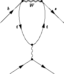
The variables ne, nw, se and sw are predefined
to the four corners of the diagram (``north-east'' etc.). In line 3
the midpoint .5[Vtb,Vts] between the V_tb and V_ts
vertices is set to the centre of the top side of the diagram. In line
4 the V_ts is defined to lie 30% of the width of the diagram
to the right of V_tb. The external b and s quarks
are set at 70% of the full height of the left and right sides of
the diagram in lines 5 and 6. The vertices p and p'
connected by the photon are defined similarly in lines 7--9. Finally,
in lines 10 and 11, the external e+, e- vertices are defined in
the same fashion as V_tb and V_ts above.
In lines 12--17 and 22--24 the straight connections are drawn, using
METAFONT's -- operator. Particularly interesting are lines 18--21 in
which METAFONT's flexible path construction primitives [3] are
used to draw the body of the penguin. The expression
Vtb{b-Vtb} .. tension 2 .. {right}p
denotes a path starting at V_tb in the
direction of the straight line connecting this vertex with the
external b quark and ending at the upper photon vertex in the
horizontal direction.
It should be noted that METAFONT's tension parameter appearing here is
unrelated to FeynMF's tension parameter. Here it is used to ``pull
in'' the arc slightly compared to the default Bezier curve which would
result in a much fatter penguin.
The diagram is completed in lines 25--28 by placing dots at all internal vertices.
In the next figure (showing Ward identities) we reproduce the figure from the bottom of page 211 of [5] is reproduced. Careful inspection will reveal that the reproduction is not faithful in one point: on the left-hand side, the doubled head of the dashed line is left out. This is easy to fix, but the most elegant solution uses FeynMF's extension mechanism and will be discussed next time.
 1 \def\F#1#2{%
 2  \fmfi{dots}{.8[vloc(__v),vloc(__#1)]
 3    -- .8[vloc(__v),vloc(__#2)]}}
 4 \def\D#1{\parbox{35mm}{%
 5 \begin{fmfgraph}(35,35)
 6  \fmfleft{s}\fmfrightn{f}{4}
 7  \fmfbottomn{b}{4}\fmfforce{c}{v}
 8  \fmfv{dec.shape=circle,dec.fill=0,
 9  	dec.size=.35w}{v}
10  \fmfv{dec.shape=tetragram,dec.fill=1,
11  	dec.size=3thick}{f3,f4,b2,b3}
12  \fmf{fermion}{f4,v,f3}
13  \fmf{fermion}{f2,v,f1}
14  \fmf{photon}{b2,v,b3}
15  \fmffreeze #1
16  \F{f1}{f2}\F{f3}{f4}\F{b2}{b3}
17 \end{fmfgraph}}}
18 \begin{multline}
19  \D{\fmf{dashes}{s,v}}\\
20  =\D{\fmfi{dashes}{%
21    vloc(__s){vloc(__v)-vloc(__s)}
22     .. .5[vloc(__s),vloc(__f4)] ..
23     {vloc(__f4)-vloc(__v)} vloc(__f4)}}\\
24  +\cdots+\D{\fmfi{dashes}{%
25    vloc(__s){vloc(__v)-vloc(__s)}
26     .. .5[vloc(__s),vloc(__f4)] ..
27    {vloc(__f3)-vloc(__v)} vloc(__f3)}}
28 \end{multline}
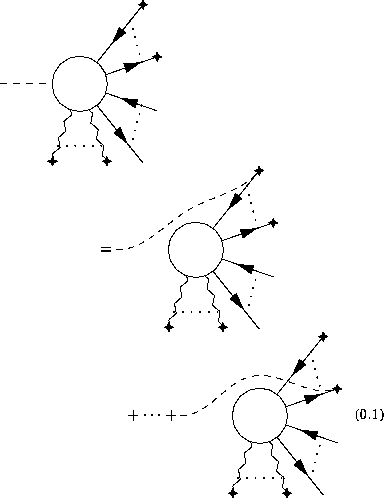
This example shows that FeynMF is very convenient for creating several structurally similar diagrams and how unusually curved lines are inserted in immediate mode. Lines 1--3 define a little macro that is used for drawing the dotted lines denoting omitted propagators. In lines 4-17 a straightforward macro is defined that sets up the common parts of the three diagrams. Note that the argument inserted after this diagram is frozen by an explicit Lcsfmffreeze. In line 18 this macro is used with another simple line. In lines 20--23 and 24--27 this simple line is replaced by two curved lines that avoid the big blob and connect external vertices.
Finally, the figure below is a slightly more advanced example: a
three-loop QCD correction to the axial vector part of the
Z0 self-energy.
 1 \begin{fmfgraph*}(50,30)
 2  \fmfleft{i} \fmfright{o}
 3  \fmf{boson,tension=2}{i,iv3}
 4  \fmf{boson,tension=2}{o,ov3}
 5  \fmf{quark}{iv1,iv2,iv3,iv1}
 6  \fmf{quark}{ov1,ov2,ov3,ov1}
 7  \fmf{gluon,tension=.5}{ov1,iv1}
 8  \fmf{gluon,tension=.5}{iv2,ov2}
 9  \fmfv{decor.shape=square,
10    decor.size=3thick}{iv3,ov3}
11  \fmfdot{iv1,iv2,ov1,ov2}
12  \fmffixed{(0,.7h)}{iv1,iv2}
13  \fmffixed{(0,.7h)}{ov1,ov2}
14  \fmffreeze
15  \fmfcmd{save loc, bmin, bmax;
16    forsuffixes $ = 1, 2, 3:
17      (loc.$.x, loc.$.y) = vloc __iv.$;
18    endfor
19    bmax.x = max(loc1x,loc2x,loc3x) + .1w;
20    bmax.y = max(loc1y,loc2y,loc3y) + .1h;
21    bmin.x = min(loc1x,loc2x,loc3x) - .1w;
22    bmin.y = min(loc1y,loc2y,loc3y) - .1h;}
23  \fmfi{dashes,width=thin}{(bmin.x,bmin.y)
24     -- (bmax.x,bmin.y) -- (bmax.x,bmax.y)
25     -- (bmin.x,bmax.y) -- cycle}
26  \fmfiv{label=$\Gamma^5_{\mu\alpha\beta}$}
27    {(.5[bmin.x,bmax.x],bmax.y)}
28 \end{fmfgraph*}
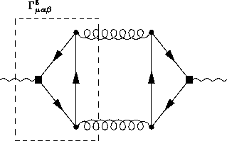
The beginning (lines 1--8) is straightforward: we
connect the vertices. It is beneficial to give a higher tension to
the bosons and a lower tension to the gluons to balance the
diagram. In lines 9--11 we add dots to the vector vertices and big
squares to the axial vector vertices. As it stands, the diagram will
have all vertices on a straight line. To remedy this situations, we
use \fmffixed to open the triangles in lines 12--13. We could also
have used phantom arcs to achieve similar results, but here the
linear constraints are more concise and intuitive.
For illustration, we mark the left triangle subgraph by a dashed box. As of version , FeynMF does not have a built-in function for calculating the enclosing box of a list of vertices. However, this is easily done in a few lines of METAFONT. Before we start, we have to force the layout calculation in line 14. For convenience, we store the coordinates of the vertices in temporary variables in lines 16--18. It is trivial to get the coordinates of the enclosing box in lines 19--22. The remaining lines use immediate mode to draw this box, thinly dashed and labelled.
This concludes our tour of FeynMF's immediate mode. In the final part of this tutorial, I will describe how to define customized line styles. Knowing how to define a bag full of new line styles should come handy if the LEP2 experiments really discover supersymmetry!