Electromagnetic Field
An Overview of Propagation in a Field
Geant4 is capable of describing and propagating in a variety of fields. Magnetic fields, electric fields, electromagnetic fields, and gravity fields, uniform or non-uniform, can specified for a Geant4 setup. The propagation of tracks inside them can be performed to a user-defined accuracy.
In order to propagate a track inside a field, the equation of motion of the particle in the field is integrated. In general, this is done using a Runge-Kutta method for the integration of ordinary differential equations. However, for specific cases where an analytical solution is known, it is possible to utilize this instead. Several Runge-Kutta methods are available, suitable for different conditions. In specific cases (such as a uniform field where the analytical solution is known) different solvers can also be used. In addition, when an approximate analytical solution is known, it is possible to utilize it in an iterative manner in order to converge to the solution to the precision required. This latter method is currently implemented and can be used particularly well for magnetic fields that are almost uniform.
Once a method is chosen that calculates the track’s propagation in a specific field, the curved path is broken up into linear chord segments. These chord segments are determined so that they closely approximate the curved path. The chords are then used to interrogate the Navigator as to whether the track has crossed a volume boundary. Several parameters are available to adjust the accuracy of the integration and the subsequent interrogation of the model geometry.
How closely the set of chords approximates a curved trajectory is governed by a parameter called the miss distance (also called the chord distance). This is an upper bound for the value of the sagitta - the distance between the ‘real’ curved trajectory and the approximate linear trajectory of the chord. By setting this parameter, the user can control the precision of the volume interrogation. Every attempt has been made to ensure that all volume interrogations will be made to an accuracy within this miss distance.
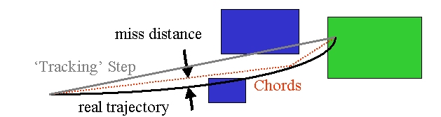
Fig. 13 The curved trajectory will be approximated by chords, so that the maximum estimated distance and chord is less than the miss distance.
In addition to the miss distance there are two more parameters which the user can set in order to adjust the accuracy (and performance) of tracking in a field. In particular these parameters govern the accuracy of the intersection with a volume boundary and the accuracy of the integration of other steps. As such they play an important role for tracking.
The delta intersection parameter is the accuracy to which an intersection with a volume boundary is calculated. If a candidate boundary intersection is estimated to have a precision better than this, it is accepted. This parameter is especially important because it is used to limit a bias that our algorithm (for boundary crossing in a field) exhibits. This algorithm calculates the intersection with a volume boundary using a chord between two points on the curved particle trajectory. As such, the intersection point is always on the ‘inside’ of the curve. By setting a value for this parameter that is much smaller than some acceptable error, the user can limit the effect of this bias on, for example, the future estimation of the reconstructed particle momentum.
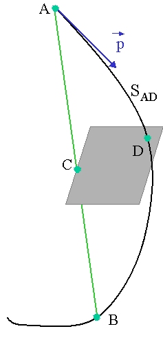
Fig. 14 The distance between the calculated chord intersection point C and a computed curve point D is used to determine whether C is an accurate representation of the intersection of the curved path ADB with a volume boundary. Here CD is likely too large, and a new intersection on the chord AD will be calculated.
The delta one step parameter is the accuracy for the endpoint of ‘ordinary’ integration steps, those which do not intersect a volume boundary. This parameter is a limit on the estimated error of the endpoint of each physics step. It can be seen as akin to a statistical uncertainty and is not expected to contribute any systematic behavior to physical quantities. In contrast, the bias addressed by delta intersection is clearly correlated with potential systematic errors in the momentum of reconstructed tracks. Thus very strict limits on the intersection parameter should be used in tracking detectors or wherever the intersections are used to reconstruct a track’s momentum.
Delta intersection and delta one step are parameters of the Field Manager; the user can set them according to the demands of his application. Because it is possible to use more than one field manager, different values can be set for different detector regions.
Note that reasonable values for the two parameters are strongly coupled: it does not make sense to request an accuracy of 1 nm for delta intersection and accept 100 \(\mu\)m for the delta one step error value. Nevertheless delta intersection is the more important of the two. It is recommended that these parameters should not differ significantly - certainly not by more than an order of magnitude.
Practical Aspects
Creating a Magnetic Field for a Detector
The simplest way to define a field for a detector involves the following steps:
create a field. It can be uniform
#include "G4SystemOfUnits.hh"

G4MagneticField *magField;
magField = new G4UniformMagField(G4ThreeVector(0.,0.,3.0*kilogauss));
or non-uniform:
magField = new G4QuadrupoleMagField( 1.*tesla/(1.*meter) );
set it as the default field:
G4FieldManager* fieldMgr
  = G4TransportationManager::GetTransportationManager()
    ->GetFieldManager();
fieldMgr->SetDetectorField(magField);
create the objects which calculate the trajectory for a pure magnetic field,:
fieldMgr->CreateChordFinder(magField);
This is a short cut, which creates all the equation of motion, a method for integration (Runge-Kutta stepper) and the driver which controls the integration and limits its estimated error.
Creating a Uniform Magnetic Field with user commands
Since 10.0 version, it is also possible to create a uniform magnetic field
and perform the other two steps above the G4GlobalMagFieldMessenger class:
G4ThreeVector fieldValue = G4ThreeVector(0.,0.,fieldValue);
fMagFieldMessenger = new G4GlobalMagFieldMessenger(fieldValue);
fMagFieldMessenger->SetVerboseLevel(1);
The messenger creates the global uniform magnetic field, which is
activated (set to the G4TransportationManager object) only when the
fieldValue is non zero vector. The messenger class setter functions
can be then used to change the field value (and activate or inactivate
the field again) or the level of output messages. The messenger also
takes care of deleting the field.
As its class name suggests, the messenger creates also UI commands which can be used to change the field value and the verbose level interactively or from a macro:
/globalField/setValue vx vy vz unit
/globalField/verbose level
Creating a Field for a Part of the Volume Hierarchy
It is possible to create a field for a part of the detector. In
particular it can describe the field (with pointer pEmField, for
example) inside a logical volume and all its daughters. This can be done
by simply creating a G4FieldManager and attaching it to a logical
volume (with pointer, logicVolumeWithField, for example) or set of
logical volumes.
G4bool allLocal = true;
logicVolumeWithField->SetFieldManager(localFieldManager, allLocal);
Using the second parameter to SetFieldManager you choose whether
daughter volumes of this logical volume will also be given this new
field. If it has the value true, the field will be assigned also to
its daughters, and all their sub-volumes. Else, if it is false, it
will be copied only to those daughter volumes
which do not have a field manager already,
and recursively to their sub-volumes without a field manager.
Creating an Electric or Electromagnetic Field
The design and implementation of the Field category allows and enables the use of an electric or combined electromagnetic field. These fields can also vary with time, as can magnetic fields.
Source listing Listing 46 shows how to define a uniform electric field for the whole of a detector.
// in the header file (or first)
#include "G4EqMagElectricField.hh"
#include "G4UniformElectricField.hh"
#include "G4DormandPrince745.hh"
...
G4ElectricField*        pEMfield;
G4EqMagElectricField*   pEquation;
G4ChordFinder*          pChordFinder ;

// in the source file

{
  pEMfield = new G4UniformElectricField(
               G4ThreeVector(0.0,100000.0*kilovolt/cm,0.0));

  // Create an equation of motion for this field
  pEquation = new G4EqMagElectricField(pEMfield);

  G4int nvar = 8;

  // Create the Runge-Kutta 'stepper' using the efficient 'DoPri5' method
  auto pStepper = new G4DormandPrince745( pEquation, nvar );

  // Get the global field manager
  auto fieldManager= G4TransportationManager::GetTransportationManager()->
       GetFieldManager();
  // Set this field to the global field manager
  fieldManager->SetDetectorField( pEMfield );

  G4double minStep     = 0.010*mm ; // minimal step of 10 microns

  // The driver will ensure that integration is control to give
  //   acceptable integration error
  auto pIntgrationDriver =
     new G4IntegrationDriver<G4DormandPrince745>(minStep,
                                                 pStepper,
                                                 nvar);

  pChordFinder = new G4ChordFinder(pIntgrationDriver);
  fieldManager->SetChordFinder( pChordFinder );
}
An example with an electric field is examples/extended/field/field02, where the class F02ElectricFieldSetup demonstrates how to set these and other parameters, and how to choose different Integration Steppers. An example with a uniform gravity field (G4UniformGravityField) is examples/extended/field/field06.
Note that using gravity since Geant4 10.6 it is necessary to enable it in the transportation process(es) used in the simulation. ( This is in order to enable optimisations which are possible only in its absence. )
The user can also create their own type of field, inheriting from
G4VField, and an associated Equation of Motion class (inheriting
from G4EqRhs) to simulate other types of fields.
How to Adjust the Accuracy of hitting a volume
Straight-line chord segments are used to detect volume boundary crossing.
The curved trajectory is broken up into such segments using an accuracy
parameter DeltaChord. Segments much be chosene so that their ‘sagitta’,
the maximum distance between the curve and chord, is smaller than DeltaChord.
So effectively this is the maximum distance by which a volume that should be
intersected could be missed.
To change the accuracy of the approximation of the curved trajectory
by linear segments, use the SetDeltaChord method:
fieldMgr->GetChordFinder()->SetDeltaChord( dcLength ); // Units: length
Geant4 propagation will seek ensure that any volume within dcLenght from the
curved trajectory will be intersected.
How to Adjust the Integration Accuracy
In order to obtain a particular accuracy in tracking particles through an electromagnetic field, it is necessary to adjust the parameters of the field propagation module. In the following section, some of these additional parameters are discussed.
When integration is used to calculate the trajectory, it is necessary to determine an acceptable level of numerical imprecision in order to get performant simulation with acceptable errors. The parameters in Geant4 tell the field module what level of integration inaccuracy is acceptable.
In all quantities which are integrated (position, momentum, energy) there will be errors. Here, however, we focus on the error in two key quantities: the position and the momentum. (The error in the energy will come from the momentum integration).
Three parameters exist which are relevant to the integration accuracy. DeltaOneStep is a distance and is roughly the position error which is acceptable in an integration step. Since many integration steps may be required for a single physics step, DeltaOneStep should be a fraction of the average physics step size. The next two parameters impose a further limit on the relative error of the position/momentum inaccuracy. EpsilonMin and EpsilonMax impose a minimum and maximum on this relative error - and take precedence over DeltaOneStep. (Note: if you set EpsilonMin=EpsilonMax=your-value, then all steps will be made to this relative precision.
G4FieldManager *globalFieldManager;

G4TransportationManager *transportMgr=
     G4TransportationManager::GetTransportationManager();

globalFieldManager = transportMgr->GetFieldManager();
                          // Relative accuracy values:
G4double minEps= 1.0e-5;  //   Minimum & value for largest steps
G4double maxEps= 1.0e-4;  //   Maximum & value for smallest steps

globalFieldManager->SetMinimumEpsilonStep( minEps );
globalFieldManager->SetMaximumEpsilonStep( maxEps );
globalFieldManager->SetDeltaOneStep( 0.5e-3 * mm );  // 0.5 micrometer

G4cout << "EpsilonStep: set min= " << minEps << " max= " << maxEps << G4endl;
We note that the relevant parameters above limit the inaccuracy in each step. The final inaccuracy due to the full trajectory will accumulate!
The exact point at which a track crosses a boundary is also calculated with finite accuracy. To limit this inaccuracy, a parameter called DeltaIntersection is used. This is a maximum for the inaccuracy of a single boundary crossing. Thus the accuracy of the position of the track after a number of boundary crossings is directly proportional to the number of boundaries.
Full control of integration method for a magnetic field
You can instead specify explicitly the full set of classes for propagating in
a magnetic field.
This provides full control over the method of integration, and allows the
choice of higher or lower order methods.
It also all you to select the use of methods which used to
be the default choice in the past (e.g. G4ClassicalRungeRK4
or G4DormandPrince745 without using interpolation.)
The classes required are the equation of motion:
auto pEquation = new G4Mag_UsualEqRhs(magField);
G4int nVar= pEquation->GetNumberOfVariables();
the method of integration (stepper):
auto pStepper = new G4DormandPrince745( pEquation );
the driver to control the accuracy of integration:
auto driver = G4InterpolationDriver<G4DormandPrince745>(minStep,pStepper, nvar);
or alternatively a driver without interpolation:
auto driver= G4IntegrationDriver<typeof(pStepper)>(minStep,pStepper, nvar);
and the chord finder:
auto chordFinder = new G4ChordFinder( driver );
Choosing a Stepper
Runge-Kutta integration is used to compute the motion of a charged track in a general field. There are many general steppers from which to choose, of low and high order, and specialized steppers for pure magnetic fields. By default, Geant4 uses the established stepper of Dormand and Prince Runge-Kutta stepper, which is general purpose, efficient and robust. It is a 5th order method which provides an error estimate directly , and requires fewer evaluations of the derivative (and field) than the previous default, the classical 4th order method (for which an error estimate required multiple sub-steps).
For somewhat smooth fields, which change smoothly over the length scales of
typical physics steps, there is choice
between fifth order steppers (such as the default G4DormandPrince745):
G4int nvar = 8;  // To integrate time & energy
                 //    in addition to position, momentum
G4EqMagElectricField* pEquation= new G4EqMagElectricField(pEMfield);

auto doPri5stepper = new G4DormandPrince745( pEquation, nvar );
  //  The recommended stepper, well suited for reasonably smooth fields
  //   and intermediate accuracy requirements ( 10^-4 to 10^-7 )
Alternative fifth order embedded steppers beside the recommended and
default G4DormandPrince745 which requires 7 field evaluations (stages)
include the older G4CashKarpRKF45 which requires fewer field evaluations
(6 ‘stages’)
auto CK45stepper = new G4CashKarpRKF45( pEquation, nvar );
   // Alternative 4/5th order stepper for reasonably smooth fields
The newest experimental classes G4BogackiShampine45 or
G4TsitourasRK45 implement some of the most efficient fifth
order methods in the literature, but require an additional derivative (field
evaluation) per step.:
auto BS45stepper = new G4BogackiShampine45( pEquation, nvar );
   // Alternative 4/5th order stepper with 8 stages (evaluations).
If there are particularly challenging accuracy demands (better than 1e-7) it may be worth to investigate higher order steppers. Alternatively, if the field is known to have specific properties, lower or higher order steppers can be used to obtain the results of the necessary accuracy using fewer computing cycles.
Since Geant4 10.5 it is recommended to use the templated driver G4IntegrationDriver together with the stepper:
auto dp45driver =
  new G4IntegrationDriver<G4DormandPrince745>(stepMin, doPri5stepper, nvar);
Steppers for rough fields
Sometimes the field changes greatly over short distances, and is estimated in ways that do not ensure that its derivatives are smooth. These can present a challenge for fourth or fifth order Runge-Kutta methods.
What matters is the variation of the field in geometrical regions in which a large fraction of particles are tracked. In particular, if the field is calculated from a field map and it varies significantly and in a non-smooth way over short distances in important regions, it is suggested to investigate a lower order stepper.
Steppers of reduced order are also suitable when lower accuracy is required, such as errors of order 10-3. Such accuracy could be suitable for the least important tracks, such as low energy electrons near the end of their trajectory (but still inside material.)
Steppers of reduced order require fewer derivative evaluations per step.
The choice of lower order steppers includes the third order embedded
stepper G4BogackiShampine23, which provides a direct error estimate.:
auto stepper = new G4BogackiShampine23( pEquation, nvar );
  //  3rd order embbedded stepper
  //  Suitable for lower accuracy needs (<~ 10^-3) and/or 'rough' fields
Older type steppers, which do not provide a direct error estimate, offer an alternative for the roughest fields. ( Note: these methods estimate the error in a step by subdividing it into two smaller steps and using the difference between the new estimate and the estimate for the whole step as the estimated error. )
The recommended ones are the fourth order G4ClassicalRK4, which was the
default in releases of Geant4 up to 10.3, and is very robust:
pStepper = new ClassicalRK4( pEquation, nvar );
    //  4th  order, the old default - a robust alternative
the third order stepper G4SimpleHeum, and the second order
steppers G4ImplicitEuler and G4SimpleRunge.:
pStepper = new G4SimpleHeum( pEquation, nvar );
    //  3rd order robust alternative for low accuracy and/or rought fields

pStepper = new G4SimpleRunge( pEquation, nvar );
    //  2nd  order, for very rough (non-smooth) fields
A first order stepper is not recommended, but may be used only for the roughest fields, as a cross check for other higher performance methods.
For somewhat smooth fields (intermediate), the choice
between a fifth order stepper (such as the default G4DormandPrince745):
pStepper = new G4DormandPrince745( pEquation, nvar );
  //  The recommended stepper, well suited for reasonably smooth fields
embedded third, the older type second or third order
steppers, or the established fourth order G4ClassicalRK4 or
should be made by trial and error.
Trying a few different types of steppers for a particular field or application is suggested if maximum performance is a goal.
The choice of stepper depends on the type of field: magnetic or general. A general field can be an electric or electromagnetic field, it can be a magnetic field or a user-defined field (which requires a user-defined equation of motion.)
For a general field all the above steppers are potential
alternatives to the recommended / default G4DormandPrince745.
But specialized steppers for pure magnetic fields are also available.
The G4NystromRK4 stepper is a fourth order method which estimates the
integration error in a step directly from the variation of the field at the
initial point, the midpoint and near the endpoint of the step.
Thus it requires no additional evaluations (stages.):
G4Mag_UsualEqRhs*
   pEquation = new G4Mag_UsualEqRhs(fMagneticField);
pStepper = new G4NystromRK4( pEquation );
Others take into account the fact that a local trajectory in a slowly varying field will not vary significantly from a helix. Combining this in with a variation the Runge-Kutta method can provide higher accuracy at lower computational cost when large steps are possible.
pStepper = new G4HelixImplicitEuler( pEquation );
// Note that for magnetic field that do not vary with time,
//  the default number of variables suffices.

// or ..
pStepper = new G4HelixExplicitEuler( pEquation );
pStepper = new G4HelixSimpleRunge( pEquation );
A new stepper for propagation in magnetic field is available in release 9.3. Choosing the G4NystromRK4 stepper provides accuracy near that of G4ClassicalRK4 (4th order) with a significantly reduced cost in field evaluation. Using a novel analytical expression for estimating the error of a proposed step and the Nystrom reuse of the mid-point field value, it requires only 2 additional field evaluations per attempted step, in place of 10 field evaluations of ClassicalRK4 (which uses the general midpoint method for estimating the step error.)
G4Mag_UsualEqRhs*
   pMagFldEquation = new G4Mag_UsualEqRhs(fMagneticField);
pStepper = new G4NystromRK4( pMagFldEquation );
It is proposed as an alternative stepper in the case of a pure magnetic field. It is not applicable for the simulation of electric or full electromagnetic or other types of field. For a pure magnetic field, results should be fully compatible with the results of ClassicalRK4 in nearly all cases. (The only potential exceptions are large steps for tracks with small momenta - which cannot be integrated well by any RK method except the Helical extended methods.)
You can choose an alternative stepper either when the field manager is constructed or later. At the construction of the ChordFinder it is an optional argument:
G4ChordFinder( G4MagneticField* itsMagField,
               G4double         stepMinimum = 1.0e-2 * mm,
               G4MagIntegratorStepper* pItsStepper = 0 );
To change the stepper at a later time use
pChordFinder->GetIntegrationDriver()
            ->RenewStepperAndAdjust( newStepper );
Increasing efficiency with interpolation and FSAL stepper
Often a significant fraction of CPU time is spent in integrating the motion of charged particles in field. This is particularly the case when the cost of evaluating the field at a location (and possibly time) is significant. To improve on this developments over the past years have introduced methods that require fewer field evaluations for the same overall accuracy.
New in Geant4 10.6 is the ability to full use of the newest RK methods, which have an interpolation capability. Such Runge-Kutta methods provide an interpolation polynomial which can be evaluated to estimate the values of all integrated variables at an arbitrary intermediate length in the integration interval.
Both these interpolation capabilities are harnessed by the new type of integration
driver G4InterpolationDriver. Currently this combination is available
only with the G4DormandPrince745 stepper.
using InterpolationDriverType = G4InterpolationDriver<G4DormandPrince745>;
auto dopri5stepper = G4DormandPrince745( pEquation, nvar );

auto interpDriver= new InterpolationDriver(stepMinimum, dopri5stepper,
                   dopri5stepper->GetNumberOfVariables() );
auto pChordFinder = new G4ChordFinder( interpDriver );
fieldManager->SetChordFinder( pChordFinder );
Geant4 10.4 introduced the capability to use RK methods with the ‘First Same as Last’ (FSAL) property. Embedded steppers with this property evaluate the field and the derivative in the equation of motion at the endpoint of each step, as an intrinsic part of the method. As a result, after a successful integration step, (one in which the estimated error was acceptable) the derivative at the start of the next step is already available. So one evaluation of the field is saved for every successive integration interval after the first one in each tracking/physical step.
Since Geant4 10.6 an FSAL capable stepper can be selected for magnetic fields
simply by requesting it when constructing a G4ChordFinder:
G4MagneticField * pMagField;
G4double  stepMinimum = 0.03 * millimeter;
G4int     useFSALstp= 1;

auto pChordFinder= new G4ChordFinder( pMagField, stepMinimum, nullptr, useFSALstp );
fieldManager->SetChordFinder( pChordFinder );
Handling very long steps by switching to helix based stepper
Very long steps of lower energy charged particles can cause excessive simulation time when regular Runge-Kutta methods are used – as these can integrate only a limited angle of a helical track in a single integration step.
This can be a problem for setups in which there is a significant fraction of tracks of low-energy charged particles in a volume with vaccum or a thin gas. In addition integration slowdown or abandoned tracks can occur when muons are tracked in a large air volume with even a fringe magnetic field.
For these setups an alternative type of driver specialised for pure magnetic fields was created. It combines an Interpolation stepper / driver for ‘shorter’ steps, and a helix-based method for ‘long’ steps.
It samples the magnetic field at the start of a step, and selects the ‘long’
step integration method if the helix angle exceed the threshold, currently
fixed at 2 pi.
This type of driver G4BFieldIntegrationDriver was the default driver
created by G4ChordFinder in Geant4 10.6 for pure magnetic fields.
G4MagneticField * pMagField;
G4double  stepMinimum = 0.03 * millimeter;
G4bool    useFSALstp= false;

auto pChordFinder= new G4ChordFinder( pMagField, stepMinimum, nullptr, useFSALstp );
fieldManager->SetChordFinder( pChordFinder );
In Geant4 10.7 the default has changed to use an interpolation driver with templated steppers (see next subsection).
As a result, to select it G4BFieldIntegrationDriver in Geant4 10.7 a user must
use:
G4int     driverId = 3;  // B-Field driver = 3
auto pChordFinder= new G4ChordFinder( pMagField, stepMinimum, nullptr, driverId );
fieldManager->SetChordFinder( pChordFinder );
It can also be created directly
using SmallStepDriver = G4InterpolationDriver<G4DormandPrince745>;
using LargeStepDriver = G4IntegrationDriver<G4HelixHeum>;

auto  regularStepper = new G4DormandPrince745(pEquation);
int   numVar = regularStepper->GetNumberOfVariables();

auto longStepper = std::unique_ptr<G4HelixHeum>(new G4HelixHeum(pEquation));

G4VIntegrationDriver driver =
  new G4BFieldIntegrationDriver(
        std::unique_ptr<SmallStepDriver>(new SmallStepDriver(stepMinimum,
                regularStepper,    numVar ) )
        std::unique_ptr<LargeStepDriver>(new LargeStepDriver(stepMinimum,
                longStepper.get(), numVar ) ) );
Speeding up using steppers templated on equation
To reduce the CPU time of field propagation in Geant4 10.7 an equation class for magnetic fields and some templated stepper classes were created.
The first optimisation is that the templated equation knows the type of the field class:
using Equation_t = G4TMagFieldEquation<Field_class_type>;
Equation_t*  equation= new Equation_t(field_object);
Given the field class’ type, the equation will invoke the field without a virtual call. The relevant include files are:
#include "G4TMagFieldEquation.hh"
#include "G4TDormandPrince45.hh"

// For field definition
#include "G4SystemOfUnits.hh"
#include "G4QuadrupoleMagField.hh"
To create the templated equation it is simpler to declare each class’ type first:
using Field_t = G4QuadrupoleMagField;
using Equation_t = G4TMagFieldEquation<Field_t>;

Field_t*     quadMagField = new G4QuadrupoleMagField(1.*tesla/(1.*meter));

Equation_t*  equation=  new Equation_t(quadMagField);
but it can also be created directly such as
auto equation= new G4TMagFieldEquation<G4QuadrupoleMagField>(quadMagField);
The second optimisation makes the type of the equation known to the templated stepper. This avoid a virtual call from the stepper to the equation.
using TemplatedStepper_t = G4TDormandPrince45<Equation_t>;

TemplatedStepper_t* dopri5_stepper=
   new G4TDormandPrince45<Equation_t>( equation );
Here G4TDormandPrince45 is the templated version of the recommended
G4DormandPrince745 stepper that implements the well known 4th/5th order embedded
Runge-Kutta method of Dormand and Prince.
Alternative methods which have a templated stepper from Geant4 10.7 include
the embedded method of Cash and Karp (G4TCashKarpRKF45), and a number of
methods which use bisection for error estimatios:
the original method of Runge and Kutta (G4TClassicalRK4) which used to
be the default before Geant4 release 10.4, and two lower order methods,
the 2nd order G4TSimpleRunge and the third order G4TSimpleHeum.
As a further optimisation, it can also be used with a templated driver
double stepMin= 0.1 * CLHEP::millimeter;

auto dp45driver =
  new G4IntegrationDriver<TemplatedStepper_t>(stepMin, dopri5_stepper);

auto interpolatingDrv =
  new G4InterpolationDriver<TemplatedStepper_t>(stepMin, dopri5_stepper);
which is simplified greatly by using a name for the type of the templated stepper.
Note that the templated stepper class also can be used without using an equation templated on the type of field. This could be preferable in the case of complex field classes in which a large amount of code calculates the value of the field.
A templated stepper also using an alternative type of field. We demonstrate using a full electromagnetic field (which in practice will be a derived class for a user’s application) and its equation G4EqMagElectricField:
#include "G4EqMagElectricField.hh"

using Equation_t = G4EqMagElectricField;
constexpr nvar= 8; //  Equation integrates over x, p, t

using TemplatedDoPri5_t = G4TDormandPrince45<Equation_t,nvar>;

MyElectroMagneticField *emField= ...; // deriving from

auto emEquation= new G4EqMagElectricField(emField);

TemplatedDoPri5_t* pStepperTDP45 = new TemplatedDoPri5_t( emEquation, nvar );

auto ck45Stepper = new G4TCashKarpRKF45<Equation_t,nvar>( emEquation, nvar );
Using different FSAL steppers – without interpolation
A different method which only has the FSAL property can be used for a magnetic field by adding a flag to the constructor of G4ChordFinder:
G4MagneticField * pMagField;
G4double  stepMinimum = 0.03 * millimeter;
G4bool    useFSALstp= true;

auto pChordF= new G4ChordFinder( pMagField, stepMinimum, nullptr, useFSALstp );
This uses the constructor:
G4ChordFinder::G4ChordFinder( G4MagneticField*        theMagField,
                              G4double                stepMinimum,
                              G4MagIntegratorStepper* pItsStepper,
                              G4bool                  useFSALstepper );
Steppers of this type can also be created directly:
#include "G4RK547FEq1.hh"
#include "G4SystemsOfUnits.hh"

using FsalStepperType = G4RK547FEq1;
G4double  stepMinimum= 0.1 * millimeter;  // Minimum size of step (for driver)
int  nvar= 6; // or 8 to include time, Energy

auto fsalStepper=  new FsalStepperType(pEquation, nvar);
They must then be coupled to a new type of driver G4FSALIntegrationDriver
in order to be used in integration.
( This is a derived class of the new base class for drivers
G4VIntegrationDriver.)
auto intgrDriver = new
     G4FSALIntegrationDriver<NewFsalStepperType>(stepMinimum,
                                                 fsalStepper,
                                                 fsalStepper->GetNumberOfVariables() );
This also demonstrates one of a new family of (FSAL) steppers G4RK547FEq1
( others are G4RK547FEq2 and G4RK547FEq3) which were created to
provide an improved equilibrium in integration.
When a integration step fails due to an error above threshold, for some
setups there can be oscillations in step size that cause multiple bounces
between a successful and a failed step.
The coefficients of these steppers were optimised to reduce these
oscillations, and thus increase the success rate of steps. Initial
tests demonstrated a small potential (1.0-2.5%) performance advantage.
Further reducing the number of field calls to speed-up simulation
An additional method to reduce the number of field evaluations is to
avoid recalculating the field value inside a sphere of a given
radius distConst from the previously evaluated location.
This can be done by utilising the class G4CachedMagneticField class, for the case of pure magnetic fields which do not vary with time.
G4MagneticField * pMagField;  // Your field - Defined elsewhere

G4double          distConst = 2.5 * millimeter;
G4MagneticField * pCachedMagField= new G4CachedMagneticField(  pMagField,  distConst);
This is not recommended if there are locations in the setup in which large variations occur in the field vector. In those cases it is best to rely on advanced integration method. In particular the Interpolation capabilities introduced in Geant4 10.6 greatly reduced the number of field calls already.
Choosing different accuracies for the same volume
It is possible to create a G4FieldManager which has different properties
for particles of different momenta (or depending on other parameters of
a track). This is useful, for example, in obtaining high accuracy for
‘important’ tracks (e.g. muons) and accept less accuracy in tracking
other tracks (e.g. electrons). To use this, you must create your own field
manager class, derived from G4FieldManager which implements the method
void ConfigureForTrack( const G4Track * ) override final;
and uses it to configure itself using the parameters of the current track.
For example to choose different values for the relative accuracy of integration for particles with energy below or above 2.5 MeV, this could be achieve as follows:
class MyFieldManager : G4FieldManager
{
  MyFieldManager() = default;
  ~MyFieldManager() = default;

  void ConfigureForTrack( const G4Track * ) override final;
};

void MyFieldManager::ConfigureForTrack( const G4Track *pTrack)
{
  const G4double lowEepsMin= 1.0e-5, lowEepsMax= 1.0e-4;
  const G4double  hiEepsMin= 2.5e-6,  hiEepsMax= 1.0e-5;

  if( pTrack->GetKineticEnergy() < 2.5 * MeV ) {
     SetMinimumEpsilonStep( lowEepsMin );
     SetMaximumEpsilonStep( lowEepsMax );  // Max relative accuracy
  } else {
     SetMinimumEpsilonStep(  hiEepsMin );
     SetMaximumEpsilonStep(  hiEepsMax );  // Max relative accuracy
  }
}
Parameters that must scale with problem size
The default settings of this module are for problems with the physical size of a typical high energy physics setup, that is, distances smaller than about one kilometer. A few parameters are necessary to carry this information to the magnetic field module, and must typically be rescaled for problems of vastly different sizes in order to get reasonable performance and robustness. Two of these parameters are the maximum acceptable step and the minimum step size.
The maximum acceptable step should be set to a distance larger than the biggest reasonable step. If the apparatus in a setup has a diameter of two meters, a likely maximum acceptable steplength would be 10 meters. A particle could then take large spiral steps, but would not attempt to take, for example, a 1000-meter-long step in the case of a very low-density material. Similarly, for problems of a planetary scale, such as the earth with its radius of roughly 6400 km, a maximum acceptable steplength of a few times this value would be reasonable.
An upper limit for the size of a step is a parameter of
G4PropagatorInField, and can be set by calling its
SetLargestAcceptableStep method.
The minimum step size is used during integration to limit the amount of work in difficult cases. It is possible that strong fields or integration problems can force the integrator to try very small steps; this parameter stops them from becoming unnecessarily small.
Trial steps smaller than this parameter will be treated with less accuracy, and may even be ignored, depending on the situation.
The minimum step size is a parameter of the MagInt_Driver, but can be set in the constructor of G4ChordFinder, as in the source listing above.
Known Issues
For most integration method it is computationally expensive to change the miss distance to very small values, as it causes tracks to be limited to curved sections whose ‘sagitta’ is smaller than this value. (The sagitta is the distance of the mid-point from the chord between endpoints see e.g. <https://en.wikipedia.org/wiki/Sagitta_%28geometry%29> .) For tracks with small curvature (typically low momentum particles in strong fields) this can cause a large number of steps
even in areas where there are no volumes to intersect (where the safety could be utilized to partially alleviate this limitation)
especially in a region near a volume boundary (in which case it is necessary in order to discover whether a track might intersect a volume for only a short distance.)
Requiring such precision for the intersection of all potential volumes is clearly expensive, and in some cases it is not possible to reduce expense greatly.
By contrast, changing the intersection parameter delta intersection is less computationally expensive. It causes further calculation for only a fraction of the steps, those that intersect a volume boundary.
Spin Tracking
The effects of a particle’s motion on the precession of its spin angular momentum in slowly varying external fields are simulated. The relativistic equation of motion for spin is known as the BMT equation. The equation demonstrates a remarkable property; in a purely magnetic field, in vacuum, and neglecting small anomalous magnetic moments, the particle’s spin precesses in such a manner that the longitudinal polarization remains a constant, whatever the motion of the particle. But when the particle interacts with electric fields of the medium and multiple scatters, the spin, which is related to the particle’s magnetic moment, does not participate, and the need thus arises to propagate it independent of the momentum vector. In the case of a polarized muon beam, for example, it is important to predict the muon’s spin direction at decay-time in order to simulate the decay electron (Michel) distribution correctly.
In order to track the spin of a particle in a magnetic field, you need to code the following:
in your DetectorConstruction:
#include "G4Mag_SpinEqRhs.hh"

G4Mag_EqRhs* pEquation = new G4Mag_SpinEqRhs(magField);
G4MagIntegratorStepper* pStepper = new G4ClassicalRK4(pEquation,12);
                                                 //    notice the 12
in your PrimaryGenerator:
particleGun->SetParticlePolarization(G4ThreeVector p)
for example:
particleGun->
SetParticlePolarization(-(particleGun->GetParticleMomentumDirection()));

// or
particleGun->
SetParticlePolarization(particleGun->GetParticleMomentumDirection()
                                       .cross(G4ThreeVector(0.,1.,0.)));
where you set the initial spin direction.
While the G4Mag_SpinEqRhs class constructor:
G4Mag_SpinEqRhs::G4Mag_SpinEqRhs( G4MagneticField* MagField )
   : G4Mag_EqRhs( MagField )
{
    anomaly = 1.165923e-3;
}
sets the muon anomaly by default, the class also comes with the public method:
inline void SetAnomaly(G4double a) { anomaly = a; }
with which you can set the magnetic anomaly to any value you require.
The code has been rewritten (in Release 9.5) such that field tracking of
the spin can now be done for charged and neutral particles with a
magnetic moment, for example spin tracking of ultra cold neutrons. This
requires the user to set EnableUseMagneticMoment, a method of the
G4Transportation process. The force resulting from the term,
MUSDOTNABLAB, is not yet implemented in Geant4 (for example, simulated
trajectory of a neutral hydrogen atom trapped by its magnetic moment in
a gradient B-field.)
Alternative Integration Methods
There are three alternative integration methods available in Geant4. One is general, can be applied for any equation of motion.
The final, Symplectic Integration, aims to preserve phase space volume and energy exactly – and its implementations achieve this to the order of the method used (currently 2nd order.)
Quantum State Simulation
The Quantum State Simulation method is a general integration method which uses polynomial approximation of the solutions of ODEs. In Geant4 its implementation is currently specialised for pure magnetic fields only. It is of potential interest to applications with a large number of volume boundary crossings per track.
#include "G4ChordFinder.hh"
#include "G4QSSDriverCreator.hh"

{
  G4MagneticField* magField = ...
  G4double  stepMinimum= 0.01 * CLHEP::mm

  auto chordFnd = new G4ChordFinder( magField, stepMinimum, nullptr, kQss2DriverType);
}
..
#include "G4QSSDriverCreator.hh"
#include "G4ChordFinder.hh"

{
    auto qssStepper2 = G4QSSDriverCreator::CreateQss2Stepper(pEquation);
    fIntgrDriver = G4QSSDriverCreator::CreateDriver(qssStepper2);

    G4cout << "-- Created QSS driver for B-field integration" << G4endl;

    auto chordFinder= new G4ChordFinder( driver );
}
..
Bulirsch-Stoer
The Bulirsch-Stoer method is an alternative to Runge-Kutta methods, and uses a midpoint method to obtain an estimate of the trajectory solution. It can be used with any equation of motion. One key use is to cross check results obtained with Runge-Kutta methods.
The current method is fourth order. (tbc)
#include "G4BulirschStoer.hh"
#include "G4BulirschStoerDriver.hh"

void DetectorConstruction::ConstructSDandField()
{
   G4MagneticField     *magField = new G4UniformMagField( G4ThreeVector( 0, 0, 3.8*tesla );
   G4EquationOfMotion  pEquation= new G4Mag_UsualEqRhs(pMyMagField);

   G4BulirschStoer  * pBSstepper = new G4BulirschStoer( pEquation, nVar, epsilon );
   G4VIntegrationDriver*  driver = new G4IntegrationDriver<G4BulirschStoer>( stepMinimum, pBSstepper, nVar );
   G4cout << "Using Bulirsch Stoer method (and driver) - alternative to RK"  << G4endl;

   G4ChordFinder*   chordFinder= new G4ChordFinder( driver );

   // Use this for the global field
   G4FieldMananger* globalFieldMgr= G4TransportationManager::GetTransportationManager()->GetFieldManager();
   globalFieldMgr->SetChordFinder( chordFinder );
}
..
Symplectic Integration
Some accelerator applications require long-term stability in the integration of energy and/or the preservation of phase-space volume. These are not well served by (medium order) Runge-Kutta method, and even high-order Runge-Kutta methods typically are not able to provide the required accuracy.
To address such applications Geant4 release 11.1 introduces a new integration
method, the symplectic 2nd order Boris integration method.
This method is implemented by the integration driver G4BorisDriver.
#include "G4BorisScheme.hh"
#include "G4BorisDriver.hh"

void
CreateBorisDriver(G4EquationOfMotion* equation,
                  G4FieldManager* fieldManager,
                  G4double minimumStep
                 )
{
  //   1. Create Scheme and Driver
  auto borisScheme = new G4BorisScheme(equation);
  auto driver = new G4BorisDriver(minimumStep, borisScheme);

  //  2. Create ChordFinder
  auto chordFinder = new G4ChordFinder( driver );

  //  3. Updating Field Manager (with ChordFinder, field)
  fieldManager->SetChordFinder( chordFinder );
}


..
Recall that in a pure magnetic field the transportation process,
e.g. G4Transportation, will conserve energy by ignoring integration errors.
The field manager stores a property ‘FieldChangesEnergy’ which recalls this,
and whose default behaviour must be overriden.
If investigating energy conservation for a pure magnetic field, you
must switch this off by calling the method
SetFieldChangesEnergy(G4bool);
with the argnument true for the relevant field manager.
This is demonstrated in the field01 extended example for the global field
manager using:
GetGlobalFieldManager()->SetFieldChangesEnergy(true);
This enables you to test the level of energy conservation in the integration.
Note in a combined electro-magnetic field this property is automatically
false, and changes due to integration already affect the particle energy.