Hadronic Physics
Introduction
Optimal exploitation of hadronic final states played a key role in successes of all recent collider experiment in HEP, and the ability to use hadronic final states will continue to be one of the decisive issues during the analysis phase of the LHC experiments. Monte Carlo programs like Geant4 facilitate the use of hadronic final states, and have been developed for many years.
We give an overview of the Object Oriented frameworks for hadronic generators in Geant4, and illustrate the physics models underlying hadronic shower simulation on examples, including the three basic types of modeling; data-driven, parametrisation-driven, and theory-driven modeling, and their possible realisations in the Object Oriented component system of Geant4. We put particular focus on the level of extendibility that can and has been achieved by our Russian dolls approach to Object Oriented design, and the role and importance of the frameworks in a component system.
Principal Considerations
The purpose of this section is to explain the implementation frameworks used in and provided by Geant4 for hadronic shower simulation as in the 1.1 release of the program. The implementation frameworks follow the Russian dolls approach to implementation framework design. A top-level, very abstracting implementation framework provides the basic interface to the other Geant4 categories, and fulfills the most general use-case for hadronic shower simulation. It is refined for more specific use-cases by implementing a hierarchy of implementation frameworks, each level implementing the common logic of a particular use-case package in a concrete implementation of the interface specification of one framework level above, this way refining the granularity of abstraction and delegation. This defines the Russian dolls architectural pattern. Abstract classes are used as the delegation mechanism 1 .
All framework functional requirements were obtained through use-case analysis. In the following we present for each framework level the compressed use-cases, requirements, designs including the flexibility provided, and illustrate the framework functionality with examples. All design patterns cited are to be read as defined in [Gamma1995] .
Level 1 Framework - processes
There are two principal use-cases of the level 1 framework. A user will want to choose the processes used for his particular simulation run, and a physicist will want to write code for processes of his own and use these together with the rest of the system in a seamless manner.
Requirements
Provide a standard interface to be used by process implementations.
Provide registration mechanisms for processes.
Design and interfaces
Both requirements are implemented in a sub-set of the tracking-physics interface in Geant4. The class diagram is shown in Fig. 33.
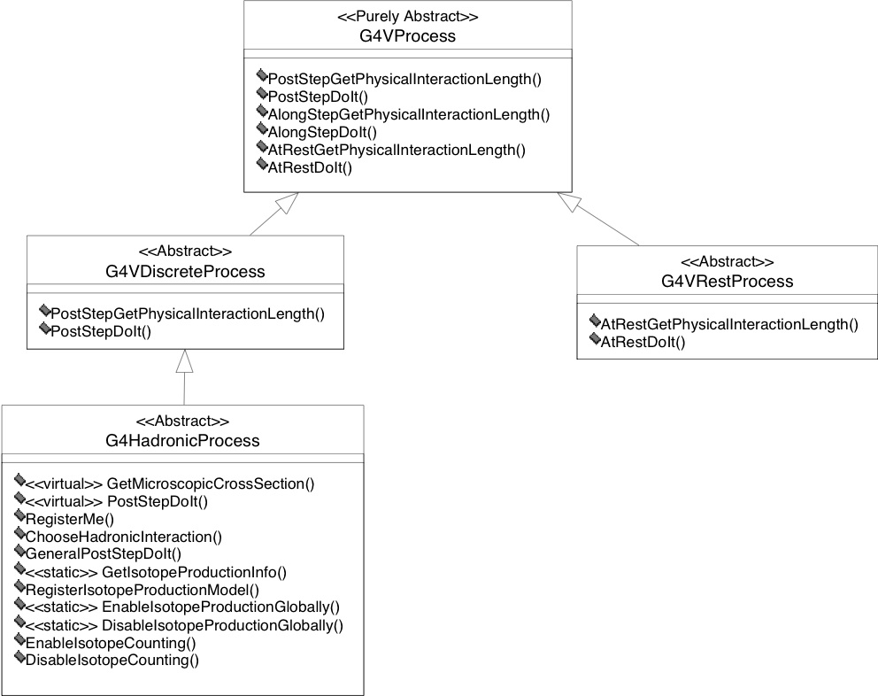
Fig. 33 Level 1 implementation framework of the hadronic category of Geant4.
All processes have a common base-class G4VProcess, from which a set
of specialised classes are derived. Two of them are used as base classes
for hadronic processes at rest and in flight (G4VDiscreteProcess),
and for processes like radioactive decay where the same implementation
can represent both these extreme cases (G4VRestDiscreteProcess).
Each of these classes declares two types of methods; one for calculating the time to interaction or the physical interaction length, allowing tracking to request the information necessary to decide on the process responsible for final state production, and one to compute the final state. These are pure virtual methods, and have to be implemented in each individual derived class, as enforced by the compiler.
Note on at-rest processes: starting with Geant4 version 9.6 - when
the Bertini and Fritiof final-state models have been extended down to
zero kinetic energy and used also for simulating the nuclear capture
at-rest - the at-rest processes derive from G4HadronicProcess, hence
from G4VDiscreteProcess, instead than from G4VRestProcess as in
the initial design of at-rest processes. This requires some adaptation a
discrete process to handle an at-rest one using top level interface
G4VProcess. A different solution, under consideration but not yet
implemented, would be instead to have G4HadronicProcess inheriting
from G4VRestDiscreteProcess: in this way, G4HadronicProcess, and
therefore any theory-driven final-state model, could be deployed for any
kind of hadronic process, including capture-at-rest processes and
radioactive decays.
Framework functionality
The functionality provided is through the use of process base-class
pointers in the tracking-physics interface, and the
G4Process-Manager. All functionality is implemented in abstract, and
registration of derived process classes with the G4Process-Manager
of an individual particle allows for arbitrary combination of both
Geant4 provided processes, and user-implemented processes. This
registration mechanism is a modification on a Chain of Responsibility.
It is outside the scope of the current paper, and its description is
available from
G4Manual.
Level 2 Framework - Cross Sections and Models
At the next level of abstraction, only processes that occur for particles in flight are considered. For these, it is easily observed that the sources of cross sections and final state production are rarely the same. Also, different sources will come with different restrictions. The principal use-cases of the framework are addressing these commonalities. A user might want to combine different cross sections and final state or isotope production models as provided by Geant4, and a physicist might want to implement his own model for particular situation, and add cross-section data sets that are relevant for his particular analysis to the system in a seamless manner.
Requirements
Flexible choice of inclusive scattering cross-sections.
Ability to use different data-sets for different parts of the simulation, depending on the conditions at the point of interaction.
Ability to add user-defined data-sets in a seamless manner.
Flexible, unconstrained choice of final state production models.
Ability to use different final state production codes for different parts of the simulation, depending on the conditions at the point of interaction.
Ability to add user-defined final state production models in a seamless manner.
Flexible choice of isotope production models, to run in parasitic mode to any kind of transport models.
Ability to use different isotope production codes for different parts of the simulation, depending on the conditions at the point of interaction.
Ability to add user-defined isotope production models in a seamless manner.
Design and interfaces
The above requirements are implemented in three framework components, one for cross-sections, final state production, and isotope production each. The class diagrams are shown in Fig. 34 for the cross-section aspects, Fig. 35 for the final state production aspects, and Fig. 36 for the isotope production aspects.

Fig. 34 Level 2 implementation framework of the hadronic category of Geant4.

Fig. 35 Level 2 implementation framework of the hadronic category of Geant4; final state production aspect.

Fig. 36 Level 2 implementation framework of the hadronic category of Geant4; isotope production aspect
The three parts are integrated in the G4Hadronic-Process class, that
serves as base-class for all hadronic processes of particles in flight.
Cross-sections
Each hadronic process is derived from G4Hadronic-Process, which
holds a list of “cross section data sets”. The term “data set” is
representing an object that encapsulates methods and data for
calculating total cross sections for a given process in a certain range
of validity. The implementations may take any form. It can be a simple
equation as well as sophisticated parameterisations, or evaluated data.
All cross section data set classes are derived from the abstract class
G4VCrossSection-DataSet, which declares methods that allow the
process inquire, about the applicability of an individual data-set
through IsApplicable(const G4DynamicParticle*, const G4Element*),
and to delegate the calculation of the actual cross-section value
through GetCrossSection(const G4DynamicParticle*, const G4Element*).
Final state production
The G4HadronicInteraction base class is provided for final state
generation. It declares a minimal interface of only one pure virtual
method:
G4VParticleChange* ApplyYourself(const G4Track &, G4Nucleus &)}.
G4HadronicProcess provides a registry for final state production
models inheriting from G4Hadronic-Interaction. Again, final state
production model is meant in very general terms. This can be an
implementation of a quark gluon string model [QGSM], a
sampling code for ENDF/B data formats [ENDFForm], or a
parametrisation describing only neutron elastic scattering off Silicon
up to 300 MeV.
Isotope production
For isotope production, a base class (G4VIsotope-Production) is
provided. It declares a method
G4IsoResult * GetIsotope(const G4Track &, const G4Nucleus &) that
calculates and returns the isotope production information. Any concrete
isotope production model will inherit from this class, and implement the
method. Again, the modeling possibilities are not limited, and the
implementation of concrete production models is not restricted in any
way. By convention, the GetIsotope method returns NULL, if the model
is not applicable for the current projectile target combination.
Framework functionality
Cross Sections
G4HadronicProcess provides registering possibilities for data sets.
A default is provided covering all possible conditions to some
approximation. The process stores and retrieves the data sets through a
data store that acts like a FILO stack (a Chain of Responsibility with a
First In Last Out decision strategy). This allows the user to map out
the entire parameter space by overlaying cross section data sets to
optimise the overall result. Examples are the cross sections for low
energy neutron transport. If these are registered last by the user, they
will be used whenever low energy neutrons are encountered. In all other
conditions the system falls back on the default, or data sets with
earlier registration dates. The fact that the registration is done
through abstract base classes with no side-effects allows the user to
implement and use his own cross sections. Examples are special reaction
cross sections of \(\mathrm{K}^0\) nuclear interactions that might be used
for \(\epsilon / \epsilon^\prime\) analysis at LHC to control the systematic error.
Final state production
The G4HadronicProcess class provides a registration service for
classes deriving from G4Hadronic-Interaction, and delegates final
state production to the applicable model.
G4Hadronic-Interaction provides the functionality needed to define
and enforce the applicability of a particular model. Models inheriting
from G4Hadronic-Interaction can be restricted in applicability in
projectile type and energy, and can be activated/deactivated for
individual materials and elements. This allows a user to use final state
production models in arbitrary combinations, and to write his own models
for final state production. The design is a variant of a Chain of
Responsibility. An example would be the likely CMS scenario - the
combination of low energy neutron transport with a quantum molecular
dynamics [QMD], invariant phase space decay
[CHIPS], and fast parametrised models for calorimeter
materials, with user defined modeling of interactions of spallation
nucleons with the most abundant tracker and calorimeter materials.
Isotope production
The G4HadronicProcess by default calculates the isotope production
information from the final state given by the transport model. In
addition, it provides a registering mechanism for isotope production
models that run in parasitic mode to the transport models and inherit
from G4VIsotope-Production. The registering mechanism behaves like a
FILO stack, again based on Chain of Responsibility. The models will be
asked for isotope production information in inverse order of
registration. The first model that returns a non-NULL value will be
applied. In addition, the G4Hadronic-Process provides the basic
infrastructure for accessing and steering of isotope-production
information. It allows to enable and disable the calculation of isotope
production information globally, or for individual processes, and to
retrieve the isotope production information through the
G4IsoParticleChange * GetIsotopeProductionInfo() method at the end
of each step. The G4HadronicProcess is a finite state machine that
will ensure the GetIsotope-ProductionInfo returns a non-zero value
only at the first call after isotope production occurred. An example of
the use of this functionality is the study of activation of a Germanium
detector in a high precision, low background experiment.
Level 3 Framework - Theoretical Models
Geant4 provides at present one implementation framework for theory driven models. The main use-case is that of a user wishing to use theoretical models in general, and to use various intra-nuclear transport or pre-compound models together with models simulating the initial interactions at very high energies.

Fig. 37 Level 3 implementation framework of the hadronic category of Geant4; theoretical model aspect.
Requirements
Allow to use or adapt any string-parton or parton transport [VNI],
Allow to adapt event generators, ex. [PYTHIA7], state production in shower simulation.
Allow for combination of the above with any intra-nuclear transport (INT).
Allow stand-alone use of intra-nuclear transport.
Allow for combination of the above with any pre-compound model.
Allow stand-alone use of any pre-compound model.
Allow for use of any evaporation code.
Allow for seamless integration of user defined components for any of the above.
Design and interfaces
To provide the above flexibility, the following abstract base classes have been implemented:
G4VHighEnergyGenerator
G4VIntranuclearTransportModel
G4VPreCompoundModel
G4VExcitationHandler
In addition, the class G4TheoFS-Generator is provided to orchestrate
interactions between these classes. The class diagram is shown in
the Fig. 37.
G4VHighEnergy-Generator serves as base class for parton transport or
parton string models, and for Adapters to event generators. This class
declares two methods, Scatter, and GetWoundedNucleus.
The base class for INT inherits from G4Hadronic-Interaction, making
any concrete implementation usable as a stand-alone model. In doing so,
it re-declares the ApplyYourself interface of
G4Hadronic-Interaction, and adds a second interface, Propagate,
for further propagation after high energy interactions. Propagate
takes as arguments a three-dimensional model of a wounded nucleus, and a
set of secondaries with energies and positions.
The base class for pre-equilibrium decay models,
G4VPre-CompoundModel, inherits from G4Hadronic-Interaction,
again making any concrete implementation usable as stand-alone model. It
adds a pure virtual DeExcite method for further evolution of the
system when intra-nuclear transport assumptions break down. DeExcite
takes a G4Fragment, the Geant4 representation of an excited nucleus,
as argument.
The base class for evaporation phases, G4VExcitation-Handler,
declares an abstract method, BreakItUP(), for compound decay.
Framework functionality
The G4TheoFSGenerator class inherits from
G4Hadronic-Interaction, and hence can be registered as a model for
final state production with a hadronic process. It allows a concrete
implementation of G4VIntranuclear-TransportModel and
G4VHighEnergy-Generator to be registered, and delegates initial
interactions, and intra-nuclear transport of the corresponding
secondaries to the respective classes. The design is a complex variant
of a Strategy. The most spectacular application of this pattern is the
use of parton-string models for string excitation, quark molecular
dynamics for correlated string decay, and quantum molecular dynamics for
transport, a combination which promises to result in a coherent
description of quark gluon plasma in high energy nucleus-nucleus
interactions.
The class G4VIntranuclearTransportModel provides registering
mechanisms for concrete implementations of G4VPreCompound-Model, and
provides concrete intra-nuclear transports with the possibility of
delegating pre-compound decay to these models.
G4VPreCompoundModel provides a registering mechanism for compound
decay through the G4VExcitation-Handler interface, and provides
concrete implementations with the possibility of delegating the decay of
a compound nucleus.
The concrete scenario of G4TheoFS-Generator using a dual parton
model and a classical cascade, which in turn uses an exciton
pre-compound model that delegates to an evaporation phase, would be the
following: G4TheoFS-Generator receives the conditions of the
interaction; a primary particle and a nucleus. It asks the dual parton
model to perform the initial scatterings, and return the final state,
along with the by then damaged nucleus. The nucleus records all
information on the damage sustained. G4TheoFS-Generator forwards all
information to the classical cascade, that propagates the particles in
the already damaged nucleus, keeping track of interactions, further
damage to the nucleus, etc.. Once the cascade assumptions break down,
the cascade will collect the information of the current state of the
hadronic system, like excitation energy and number of excited particles,
and interpret it as a pre-compound system. It delegates the decay of
this to the exciton model. The exciton model will take the information
provided, and calculate transitions and emissions, until the number of
excitons in the system equals the mean number of excitons expected in
equilibrium for the current excitation energy. Then it hands over to the
evaporation phase. The evaporation phase decays the residual nucleus,
and the Chain of Command rolls back to G4TheoFS-Generator,
accumulating the information produced in the various levels of
delegation.
Level 4 Frameworks - String Parton Models and Intra-Nuclear Cascade
The use-cases of this level are related to commonalities and detailed choices in string-parton models and cascade models. They are use-cases of an expert user wishing to alter details of a model, or a theoretical physicist, wishing to study details of a particular model.
Requirements
Allow to select string decay algorithm
Allow to select string excitation.
Allow the selection of concrete implementations of three-dimensional models of the nucleus
Allow the selection of concrete implementations of final state and cross sections in intra-nuclear scattering.
Design and interfaces
To fulfill the requirements on string models, two abstract classes are
provided, the G4VParton-StringModel and the
G4VString-Fragmentation. The base class for parton string models,
G4VParton-StringModel, declares the GetStrings() pure virtual
method. G4VString-Fragmentation, the pure abstract base class for
string fragmentation, declares the interface for string fragmentation.
To fulfill the requirements on intra-nuclear transport, two abstract
classes are provided, G4V3DNucleus, and G4VScatterer. At this
point in time, the usage of these intra-nuclear transport related
classes by concrete codes is not enforced by designs, as the details of
the cascade loop are still model dependent, and more experience has to
be gathered to achieve standardisation. It is within the responsibility
of the implementers of concrete intra-nuclear transport codes to use the
abstract interfaces as defined in these classes.
The class diagram is shown in Fig. 38 for the string parton model aspects, and in Fig. 39 for the intra-nuclear transport.
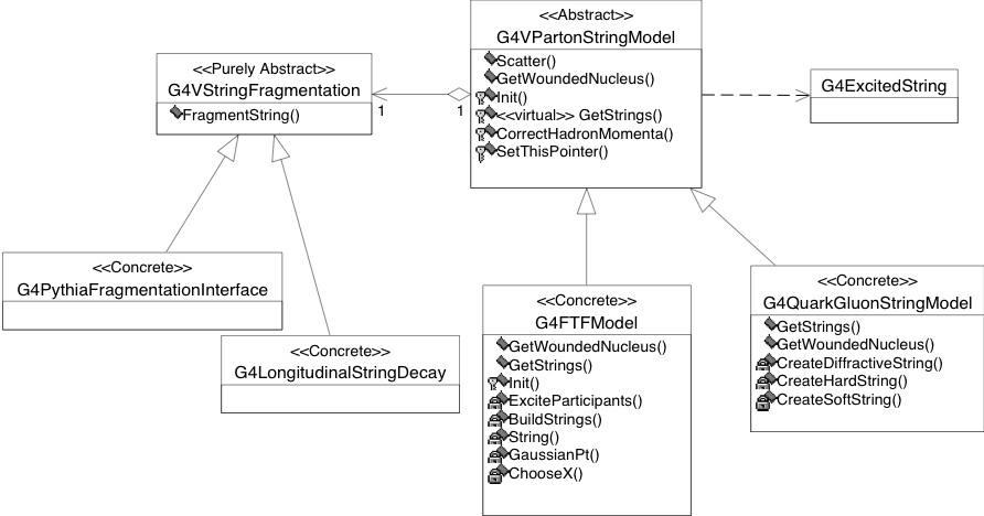
Fig. 38 Level 4 implementation framework of the hadronic category of Geant4; parton string aspect.

Fig. 39 Level 4 implementation framework of the hadronic category of Geant4; intra-nuclear transport aspect.
Framework functionality
Again variants of Strategy, Bridge and Chain of Responsibility are used.
G4VParton-StringModel implements the initialisation of a
three-dimensional model of a nucleus, and the logic of scattering. It
delegates secondary production to string fragmentation through a
G4VString-Fragmentation pointer. It provides a registering service
for the concrete string fragmentation, and delegates the string
excitation to derived classes. Selection of string excitation is through
selection of derived class. Selection of string fragmentation is through
registration.
Level 5 Framework - String De-excitation
The use-case of this level is that of a user or theoretical physicist wishing to understand the systematic effects involved in combining various fragmentation functions with individual types of string fragmentation. Note that this framework level is meeting the current state of the art, making extensions and changes of interfaces in subsequent releases likely.
Requirements
Allow the selection of fragmentation function.
Design and interfaces
A base class for fragmentation functions,
G4VFragmentation-Function, is provided. It declares the
GetLightConeZ() interface.
Framework functionality
The design is a basic Strategy. The class diagram is shown in
Fig. 40. At this point in time, the
usage of the G4VFragmentation-Function is not enforced by design,
but made available from the G4VString-Fragmentation to an
implementer of a concrete string decay. G4VString-Fragmentation
provides a registering mechanism for the concrete fragmentation
function. It delegates the calculation of zf of the hadron to
split of the string to the concrete implementation. Standardisation in
this area is expected.
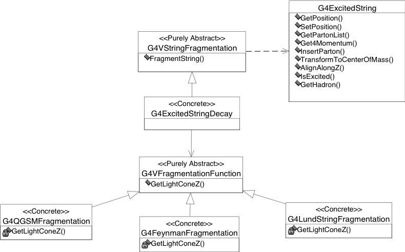
Fig. 40 Level 5 implementation framework of the hadronic category of Geant4; string fragmentation aspect.
Creating Your Own Hadronic Process
For some applications Geant4 might not provide the most appropriate physics implementation or, in fact, any physics implementation at all. In such cases, it is up to the user to develop the necessary processes, models and cross sections and integrate them into his version of the Geant4 toolkit. The user’s process, model or cross section may then be used in a physics list to replace some of those already provided by the toolkit. This modularity requires that user classes be derived from a set of base classes which have been provided to aid integration with the toolkit and to spare the user from consideration of many details not related to the physics at hand.
Processes communicate with Geant4 tracking, telling it where or when an interaction is supposed to occur, and what is supposed to happen at that point. A hadronic process may be implemented directly, or through the use of a framework of classes that modularize physics functionality, make available several utilities and reduce unnecessary code duplication. In the latter, recommended, approach the user must in general develop as many as three classes: a process, a cross section and a model. Instances of the cross section and model classes must then be assigned to the process. In practice it is usually necessary to develop only a model class or a cross section class, since a number of processes are already provided by Geant4. Before writing any code, users should check that Geant4 has not already provided the necessary models, cross sections or processes.
Developing a new hadronic model
A hadronic model is responsible for the generation of a set of final state four-vectors, given an initial projectile and target. New models should derive from the G4HadronicInteraction base class and at least two methods in this class must be implemented:
virtual G4HadFinalState*
ApplyYourself(const G4HadProjectile& aProjectile, G4Nucleus& targetNucleus)
which is responsible for generating the final state of the interaction including the specification of all particle types and four-momenta, and
virtual G4bool IsApplicable(const G4HadProjectile& aProjectile, G4Nucleus& targetNucleus)
which is responsible for checking that the incident particle type and energy, and the Z and A of the target nucleus, can be adequately handled by the model. G4HadronicInteraction provides a number of utilities to aid in the implementation of these methods.
When implementing ApplyYourself(), the Get() methods of the G4HadProjectile and G4Nucleus classes provide all the initial state information necessary for the generation of the final state. For G4HadProjectile, GetDefinition() provides the particle type, and Get4Momentum() provides the total energy and momentum. For G4Nucleus, GetZ_asInt(), GetN_asInt() and GetA_asInt() provide Z, N and A, while AtomicMass() provides the mass. Additional utility methods are available for both G4HadProjectile and G4Nucleus .
Coordinate systems
The inputs to the model assume that the incident particle (G4HadProjectile) travels along the z axis and interacts with the target (G4Nucleus) which is at rest in the lab frame. Before invoking the ApplyYourself() method, the process rotates the direction of the projectile to be along the z axis and then performs the inverse rotation on the final state particles produced by the model.
The model must perform two additional transformations: into the CM frame, and back out of it after the interaction is complete.
Writing the ApplyYourself() method
It is thus the model developer’s responsibility to:
boost the projectile and target into the CM frame using the necessary Lorentz transformations,
perform all calculations required to generate the final state set of particles,
boost the final state particles back to the lab frame with the inverse transformation, and
send the final state particles to the process by filling G4HadFinalState and setting its status.
Step 4) is accomplished by using the various Get() and Set() methods provided by the class G4HadFinalState. The developer must also decide whether the original projectile survives the interaction, disappears or is suspended. This is done with the SetStatusChange() method. If the projectile survives, the change in its energy and momentum must be set with the provided methods and it must be flagged as “isAlive”. If the particle disappears it must be flagged as “stopAndKill”.
Geant4 provides a large number of Lorentz transformation tools which may be used to complete steps 1) and 3).
How step 2) is accomplished is entirely up to the developer. This could be as simple as a look-up table which assigns a final state to an initial state, or as complex as a theoretical high energy generator. Typically, the user will have to provide methods of sampling final state multiplicities, energies and angles using random number generators provided by Geant4. For example, the cosine of the polar angle of an isotropic angular distribution could be sampled as follows:
G4double cosTheta = 2.*G4UniformRandom() - 1.;
The developer must also see to it that the model conserves energy and momentum. Currently the hadronic framework checks that final states do not exceed reasonably small limits of non-conservation.
Using the hadronic framework
For complex models it is recommended that the user become familiar with the Geant4 hadronic framework. This is covered in detail in the chapter on Extended Functionality in this manual. The framework uses the object-oriented principles of abstraction and re-use to provide a number of services to the developer. The part of the framework used will depend on the type of model. For example, high energy models can take advantage of already-developed string excitation and decay functions and medium energy models can use the intra-nuclear propagation base class and the nuclear de-excitation handler.
Writing the IsApplicable() method
The is a straightforward, but important, method. Most models are quite specific in their range of use and the developer must codify this. It is recommended that this method test for ranges of projectile energy, particle type and target atomic number and weight, and return false when these ranges are exceeded.
Developing a new cross section set
New cross section sets should derive from G4VCrossSectionDataSet . This class serves as a container of cross section data and provides a number of access methods that must be implemented by the developer. The essential methods are:
G4double GetElementCrossSection(const G4DynamicParticle*, G4int Z)
which retrieves element-based cross sections,
G4double GetIsoCrossSection(const G4DynamicParticle*, G4int Z, G4int A)
which retrieves isotope-based cross sections,
G4bool IsElementApplicable(const G4DynamicParticle*, G4int Z)
which sets the Z range of the element-based data set,
G4bool IsIsoApplicable(const G4DynamicParticle*, G4int, G4int A)
which sets the Z and A range of the isotope-based data set, and
SetMinKinEnergy(G4double)
SetMaxKinEnergy(G4double)
GetMinKinEnergy()
and GetMaxKinEnergy()
for defining the applicable energy range of the data set.
Developing a new hadronic process
As mentioned above, it is preferable to add new physics in terms of a model, and assign the model to an existing process, rather than develop a new, specific process. Under certain circumstances though, a directly implemented process may be necessary. In that case it must derive from G4HadronicProcess and three methods of that class must be implemented:
virtual G4VParticleChange* PostStepDoIt(const G4Track&, const G4Step&) ,
virtual G4bool IsApplicable(const G4ParticleDefinition&) , and
G4double GetMeanFreePath(const G4Track& aTrack, G4double, G4ForceCondition*).
PostStepDoIt() is responsible for generating the final state of an interaction given the track and step information. It must update the state of the track, flagging it as “Alive”, “StopButAlive”, “StopAndKill”, “KillTrackAndSecondaries”, “Suspend”, or “PostponeToNextEvent”. It is roughly analogous to the ApplyYourself() method in models.
IsApplicable() serves the same purpose in processes as it does in models.
GetMeanFreePath() gets the cross section as a function of particle type, energy, and target material, and converts it to a mean free path, which is in turn passed on to the tracking. This method can be quite simple:
G4double particle = aTrack.GetDynamicParticle();
G4double material = aTrack.GetMaterial();
return factor/theCrossSectionDataStore->GetCrossSection(particle, material);
provided an appropriate cross section data set is already available in the data store.
The above discussion refers to in-flight processes. At-rest hadronic processes do not currently derive from G4HadronicProcess, but from G4VRestProcess or G4VRestDiscreteProcess. As such they do not employ the full hadronic framework and must be implemented directly without models. The methods to be implemented are similar to those in the in-flight case:
virtual G4VParticleChange* AtRestDoIt(const G4Track&, const G4Step&) , and
G4bool IsApplicable(const G4ParticleDefinition&) .
Changing Internal Parameters of an Existing Hadronic Model
For the advanced user, it is possible to change the internal parameters of a hadronic model. This may be useful to understand the systematic contribution of individual settings with respect to macroscopic outcomes. Although offering insight it is strongly advised to maintain the default settings for the provided models. These values were obtained through theoretical insight from the model developers as well as extensive validation against thin target data. The user is reminded of the following warning should changes be introduced to these essentially internal parameters:
Warning
Changing these parameters without the guidance of the model developers may significantly alter or even degrade the model’s physics performance. Any publication based on varied parameters must explicitly state what those values are, along with the physics list used and the Geant4 version.
As an example of how to modify modelling at an internal microscopic level we describe here the available interfaces to the Bertini cascade model (Advanced Interface to Change the Parameters of the Bertini Cascade Model) and the FTF model (Advanced Interface to Change the Parameters of the Fritiof (FTF) Model). For illustration, we include the actual blocks of code and the physical objects they represent where applibable (Changing internal parameters of an existing model: Fritiof (FTF) use-case and Changing parameters of an existing model: Lund use-case).
Advanced Interface to Change the Parameters of the Bertini Cascade Model
This section provides a list of the configurable parameters and switches currently used in the Geant4 Bertini cacade model, along with explanations of their meaning. Guidelines are provided for changing these parameters in order to study the sensitivity of the model’s predictions. The interface, in its current format, is available since release series 10.1.
Parameters which can be changed
Parameters have already been determined to produce the best overall description of the validation data sets used by Geant4. These are referred to as “default” parameters and are listed below.
Currently the Bertini cascade model does not have a traditional C++ configuration interface. Instead its configuration interface is implemented in a form of Geant4 UI commands. Such commands may be used in a configuration macrofile on input to a Geant4 application.
With regards to this, one should bear in mind the following:
Changes of Bertini Cascade parameters must be made before a physics list is instantiated since the parameters are taken into account when Bertini Cascade constructor is called.
However, there is currently no guaranteed way to uniformly specify the Bertini cascade parameters and switches, the physics list, and a variety of other G4UI options in a single job configuration macro, or to ensure a particular order of their execution. This will be the subject of further development and is outside the scope of this document. At present it is better to collect all desired Bertini cascade configuration cards in a dedicated job configuration macro and to ensure that such macro is processed very early in the workflow.
Alternatively, the Bertini cascade configuration commands can be used in the Geant4 application
C++ code, via the ApplyCommand function of the G4UImanager singleton which belongs to
the geant4/source/intercoms domain.
As mentioned above, the changes to Bertini cascade parameters should be made very early in the job, in order to custom settings to propagate.
The application should be in the G4State_PreInit state; otherwise changes to Bertini cascade
model parameters will not propagate, and there is no guarantee of a warning message to this effect
(it is also possible to use Idle state but PreInit is the recommended one).
The following UI commands (case sensitive) represent the most “sensitive” parameters and switches:
/process/had/cascade/crossSectionScale <value> - multiplicative factor applied to the internal cross sections used in Bertini model of the nucleus; DEFAULT=1; Limits: 0.05-2.0 Here “internal” means the cross section that an insident particicle sees as it travels through the target nucleus; it is not the free space cross section. Typical changes in output spectra over the allowed range can be as large as a factor of 2-3, and the shapes of the spectra may change as well.
/process/had/cascade/nuclearRadiusScale <value> - multiplicative factor applied to the nuclear radius; DEFAULT=2.82; Limits: 1.0-2.82 Currently the nuclear radius used in Bertini is 2.82 times the radius measured from electron scattering. Increasing (decreasing) this parameter will increase (decrease) the nuclear volume and thus decrease (increase) the nuclear density. Over the allowed range a factor of 2 change in the output spectra is possible.
/process/had/cascade/fermiScale <value> - adjusts Fermi momentun of bound nucleons by multiplying it by the above factor; DEFAULT=0.685; Limits: 0.5-1.0 Increasing (decreasing) this value will change the depth of the nuclear potential seen by protons and neutrons in the nucleus. This in turn would increase (decrease) the energy of target nucleons in the nucleus and similarly alter the energy of produced nucleon secondaries. Though not as sensitive as the cross section and radius parameters, variations of the parameter over this range will produce noticeable changes in the mean energy of outgoing nucleons.
/process/had/cascade/shadowingRadius <value> - the so called trailing effect takes into account the local depletion of nuclear density following an intra-nuclear collision; DEFAULT=0.; Limits: 0.-2.0 Increasing (decreasing) this value decreases (increases) the likelihood of secondaries being produced. A value of 0 completely neglects the effect, and a value between 0.7 and 1.0 coresponds to the effective size of a nucleon.
/process/had/cascade/usePreCompound 0/1 - switches between Bertini cascade’s native deexcitation model and the Geant4 PreCompound model; DEFAULT=0 (false) In some cases switching to PreCompound model may give more accurate results. However, some CPU penatly is not excluded.
/process/had/cascade/doCoalescence 0/1 - single nucleons that escape the nucleus after the intra-nuclear cascade are groupped together into deuterons, 3He, tritons, or alphas; DEFAULT=1 (true) This is done to make up a deficit of these particles at energy scales above the evaporation spectra.
/process/had/cascade/usePhaseSpace 0/1 - switch between Bartini cascade’s native phase-space generator and Kopylov phase-space generator; DEFAULT=0 (false)
/process/had/cascade/gammaQuasiDeutScale <value> - miltiplicative factor applied to the cross section of the process of an intra-nuclear pion absorption on a pair of nucleons that momentarily come close together; DEFAULT=1.0; Limits: 0.5-2.0 This is relevant only to modeling gamma-nuclear interactions. When embedded in a nucleus this cross section is not well-known, but a parameter value of 1.0 corresponds to its free-space value. The effect of such variations could be significant, but not many studies have been done.
Additional parameters and switches are the following:
/process/had/cascade/piNAbsorption <value> - pion absorption on nucleon below certain energy E(\(GeV\)); DEFAULT=0. \(GeV\)
/process/had/cascade/use3BodyMom 0/1 - use 3-body momentum parametrizations; DEFAULT=0 (false)
/process/had/cascade/useTwoParamNuclearRadius 0/1 - calculate nuclear radius as \(R = C_{1}*A^{1/3} + C_{2}/A^{1/3}\); DEFAULT=0 (false)
/process/had/cascade/smallNucleusRadius <value> - fixed radius for light ions (A<4); DEFAULT=8.0
/process/had/cascade/alphaRadiusScale <value> - fraction of light-ion radius for alphas; DEFAULT=0.7
/process/had/cascade/cluster2DPmax <value> - momentum cut in \(GeV\) for \(pn \rightarrow D\); DEFAULT=0.09 \(GeV\)
/process/had/cascade/cluster3DPmax <value> - momentum cut in \(GeV\) for \(pnn \rightarrow T\), DEFAULT=0.108 \(GeV\)
/process/had/cascade/cluster4DPmax <value> - momentum cut in \(GeV\) for \(ppnn \rightarrow alpha\); DEFAULT=0.115 \(GeV\)
While Bertini cascade configuration interface does not allow to change model’s parameters
in the programmatic C++ way, there is still a possibility to print out desired settings,
e.g. to compare the value of a given parameter before and after the modification.
This can be done with the use of the G4CascadeParameters singleton that belongs to the
geant4/source/processes/hadronic/models/cascade/cascade.
Example usage in a C++ application code:
#include "G4UImanager.hh"
#include "G4StateManager.hh"
#include "G4CascadeParameters.hh"
G4CascadeParameters* bpars = G4CascadeParameters::Instance();
G4cout << " Bertini default: RadiusScale = " << bpars->radiusScale() << G4endl;
G4cout << " Bertini default: UsePreCo = " << bpars->usePreCompound() << G4endl;
G4ApplicationState currentstate = G4StateManager::GetStateManager()->GetCurrentState();
bool ok = G4StateManager::GetStateManager()->SetNewState(G4State_PreInit);
if ( ok )
{
   G4UImanager* UIM = G4UImanager::GetUIpointer();
   uim->ApplyCommand("/process/had/cascade/nuclearRadiusScale 1.5");
   uim->ApplyCommand( "/process/had/cascade/usePreCompound 1" );
   G4cout << " After changes: RadiusScale = " << bpars->radiusScale() << G4endl;
   G4cout << " After changes: UsePreCo = " << bpars->usePreCompound() << G4endl;
}
else
{
   G4cout << " G4StateManager PROBLEM: can NOT change state to G4State_PreInit !" << G4endl;
   G4cout <<
   " Bertini cascade parameters can not be changed unless in the G4State_PreInit state !"
   << G4endl;
}
ok = G4StateManager::GetStateManager()->SetNewState( currentstate );
Last but not least, please pay attention to the order of calls in the above example.
Due to implementation details, it is important to anyhow call G4CascadeParameters::Instance()
before applying any changes; otherwise all changes will be overriden by the default settings
of the Bertini cascade model.
Advanced Interface to Change the Parameters of the Fritiof (FTF) Model
This section provides a list of the configurable parameters and switches currently used in the Geant4 Fritiof model (FTF), along with explanations of their meaning and effect on the final state hadron production of the model. The interface was first introduced in release 10.4, however the functionality, as described in this document, is only available starting with the release series 10.6. Guidelines are provided for changing these parameters in order to study the sensitivity of the model’s predictions. More detailed information about the roles that these parameters play in the model is also provided later in this document, see Changing internal parameters of an existing model: Fritiof (FTF) use-case.
Parameters which can be changed
Parameters have already been determined to produce the best overall description of the validation data sets used by Geant4. These are referred to as “default” parameters and are listed below.
At present, only a group of parameters and switches involved in modeling interactions of baryons or pions with nuclei has been made configurable. Other use-cases may follow in the future. For this reason most of the names of the parameters contains either “BARYON” or “PION” notation. However, some of the parameters are common for different types of meson projectile (not only pions); those parameters contain “MESON” in their names.
Parameters can be varied with the use of G4HadronicDeveloperParameters singleton which belongs
to the /geant4/source/processes/hadronic/util domain of the Geant4 source code.
Example usage:
#include "G4HadronicDeveloperParameters.hh"
G4HadronicDeveloperParameters& HDP = G4HadronicDeveloperParameters::GetInstance();
Please bear in mind that when a parameter is modified, a warning message is produced stating that the value has changed from the default one.
Parameters to control projectile or target diffraction dissociation
In general, the results of hadron-hadron interaction modeled by FTF are hadrons in the excited state. If one of the final hadrons is in the ground state, the reaction is called “single diffraction dissociation”. If none of the final hadrons is in the ground state (i.e. all are excited), it is called “non-diffractive” interaction. The excited hadrons are treated as QCD strings that further decay through the fragmentation mechanism.
The following parameters are involved in modeling excitation of the participating hadron as a QCD string:
FTF_BARYON_DELTA_PROB_QEXCHG - for baryon projectile, the probability of one or two final particles to be in the Delta-resonance state due to the quark exchange without excitation of the participating hadrons; DEFAULT=0.
FTF_PION_DELTA_PROB_QEXCHG - similar to the above, for pion projectile; DEFAULT=0.56
FTF_BARYON_PROB_SAME_QEXCHG - the probability of the same quark exchange between interacting hadrons; DEFAULT=0.0
FTF_BARYON_DIFF_M_PROJ - for baryon projectile, threshold for the excited string mass sampling for the projectile hadron in the diffractive interactions; DEFAULT=1.16 \(GeV\); Limits: 1.16 - 3.0 \(GeV\)
FTF_PION_DIFF_M_PROJ - similar to the above, for pion projectile; DEFAULT=1. \(GeV\); Limits: 0.5 - 3.0 \(GeV\)
FTF_BARYON_NONDIFF_M_PROJ - for baryon projectile, threshold for the excited string mass sampling for the projectile hadron in the non-diffractive interactions; DEFAULT=1.16 \(GeV\); Limits: 1.16 - 3.0 \(GeV\)
FTF_PION_NONDIFF_M_PROJ - similar to the above, for pion projectile; DEFAULT=1. \(GeV\); Limits: 0.5 - 3.0 \(GeV\)
FTF_BARYON_DIFF_M_TGT - for baryon projectile, threshold for the excited string mass sampling for the target hadron in the diffractive interactions; DEFAULT=1.16 \(GeV\); Limits: 1.16 - 3.0 \(GeV\)
FTF_PION_DIFF_M_TGT - similar to the above, for pion projectile; DEFAULT=1.16 \(GeV\); Limits: 1.16 - 3.0 \(GeV\)
FTF_BARYON_NONDIFF_M_TGT - for baryon projectile, threshold for the excited string mass sampling for the target hadron in the non-diffractive interactions; DEFAULT=1.16 \(GeV\); Limits: 1.16 - 3.0 \(GeV\)
FTF_PION_NONDIFF_M_TGT - similar to the above, for pion projectile; DEFAULT=1.16 \(GeV\); Limits: 1.16 - 3.0 \(GeV\)
FTF_BARYON_AVRG_PT2 - for baryon projectile, average transverse momentum squared in the excitation process; DEFAULT=0.3 \((GeV/c)^2\); Limits: 0.08 - 1.0 \((GeV/c)^2\)
FTF_PION_AVRG_PT2 - similar to the above, for pion projectile; DEFAULT=0.3 \((GeV/c)^2\); Limits: 0.08 - 1.0 \((GeV/c)^2\)
Example usage:
G4HadronicDeveloperParameters& HDP = G4HadronicDeveloperParameters::GetInstance();
HDP.Set( "FTF_BARYON_NONDIFF_M_PROJ", 2.5 );
HDP.Set( "FTF_BARYON_AVRG_PT2", 0.75 );
HDP.Set( "FTF_PION_NONDIFF_M_PROJ", 0.75 );
HDP.Set( "FTF_BARYON_AVRG_PT2", 0.6 );
By default, diffraction is switched OFF for both projectile or target. This can be changed with the use of the following Boolean switches, e.g.:
HDP.Set( "FTF_BARYON_DIFF_DISSO_PROJ", true );
HDP.Set( "FTF_BARYON_DIFF_DISSO_TGT", true );
HDP.Set( "FTF_PION_DIFF_DISSO_PROJ", true );
HDP.Set( "FTF_PION_DIFF_DISSO_TGT", true );
Additionally, as described in greater details later in this document, FTF implementatuon includes modeling of such processes as quark exchange with or whithout excitation of participant. Probability of each such processes is calculated according to the following formula:
where \(y\) is the projectile rapidity in the target rest frame, and A’s and B’s are numeric parameters that can be configured at run time. Please be careful here, and bear in mind that these parameters are likely to be correlated. Work in currently in progress to better determine correlations among parameters and their validity ranges. Additional information on this matter will be offered as soon as it becomes available.
Internally within FTF these processes are numbered as process zero, one, etc., thus parameters involved in the calculations have in their names notations such as “PROC0” or similar. Calculating probability for quark exchange with excitation of participant also involes an additional multiplier that is also calculated by the above mentioned formula; internally it is numbered as process number four, thus corresponding parameters have “PROC4” in their names.
The list of these configurable parameters is the following:
FTF_BARYON_PROC0_A1 - for baryon projectile, the A1 in the probability formula for quark exchange without excitation; DEFAULT=13.71
FTF_PION_PROC0_A1 - similar to the above for pion projectile; DEFAULT=150.0
FTF_BARYON_PROC0_B1 - for baryon projectile, B1 in the probability formula for quark exchange without excitation; DEFAULT=1.75
FTF_PION_PROC0_B1 - similar to the above for pion projectile; DEFAULT=1.8
FTF_BARYON_PROC0_A2 - for baryon projectile, the A2 in the probability formula for quark exchange without excitation; DEFAULT=-30.69
FTF_PION_PROC0_A2 - similar to the above for pion projectile; DEFAULT=-247.3
FTF_BARYON_PROC0_B2 - for baryon projectile, the B2 in the probability formula for quark exchange without excitation; DEFAULT=3.0
FTF_PION_PROC0_B2 - similar to the above for pion projectile; DEFAULT=2.3
FTF_BARYON_PROC0_A3 - for baryon projectile, the A3 in the probability formula for quark exchange without excitation; DEFAULT=0.0
FTF_PION_PROC0_A3 - similar to the above for pion projectile; DEFAULT=0.0
FTF_BARYON_PROC0_ATOP - for baryon projectile, probability of quark exchange without excitation in case projectile rapidity is less than YMIN (see below); DEFAULT=1.0
FTF_PION_PROC0_ATOP - similar to the above for pion projectile; DEFAULT=1.0
FTF_BARYON_PROC0_YMIN - for baryon projectile, if the projectile rapidity is below this threshold, probability of quark exchange without excitation is set to ATOP (see above); DEFAULT=0.93
FTF_PION_PROC0_YMIN - similar to the above for pion projectile; DEFAULT=2.3
FTF_BARYON_PROC1_A1 - for baryon projectile, the A1 in the probability formula for quark exchange with excitation; DEFAULT=25.0
FTF_PION_PROC1_A1 - similar to the above for pion projectile; DEFAULT=5.77
FTF_BARYON_PROC1_B1 - for baryon projectile, the B1 in the probability formula for quark exchange with excitation; DEFAULT=1.0
FTF_PION_PROC1_B1 - similar to the above for pion projectile; DEFAULT=0.6
FTF_BARYON_PROC1_A2 - for baryon projectile, the A2 in the probability formula for quark exchange with excitation; DEFAULT=-50.34
FTF_PION_PROC1_A2 - similar to the above for pion projectile; DEFAULT=-5.77
FTF_BARYON_PROC1_B2 - for baryon projectile, the B2 in the probability formula for quark exchange with excitation; DEFAULT=1.5
FTF_PION_PROC1_B2 - similar to the above for pion projectile; DEFAULT=0.8
FTF_BARYON_PROC1_A3 - for baryon projectile, the A3 in the probability formula for quark exchange with excitation; DEFAULT=0.0
FTF_PION_PROC1_A3 - similar to the above for pion projectile; DEFAULT=0.0
FTF_BARYON_PROC1_ATOP - for baryon projectile, probability of quark exchange with excitation in case projectile rapidity is less than YMIN (see below); DEFAULT=0.0
FTF_PION_PROC1_ATOP - similar to the above for pion projectile; DEFAULT=0.0
FTF_BARYON_PROC1_YMIN - for baryon projectile, if the projectile rapidity is below this threshold, probability of quark exchange with excitation is set to ATOP (see above); DEFAULT=1.4
FTF_PION_PROC1_YMIN - similar to the above for pion projectile; DEFAULT=0.0
FTF_BARYON_PROC4_A1 - for baryon projectile, the A1 in the probability formula that determines additional multiplier for quark exchange with excitation; DEFAULT=0.6
FTF_PION_PROC4_A1 - similar to the above for pion projectile; DEFAULT=1.0
FTF_BARYON_PROC4_B1 - for baryon projectile, the B1 in the probability formula that determines additional multiplier for quark exchange with excitation; DEFAULT=0.0
FTF_PION_PROC4_B1 - similar to the above for pion projectile; DEFAULT=0.0
FTF_BARYON_PROC4_A2 - for baryon projectile, the A2 in the probability formula that determines additional multiplier for quark exchange with excitation; DEFAULT=-1.2
FTF_PION_PROC4_A2 - similar to the above for pion projectile; DEFAULT=-11.02
FTF_BARYON_PROC4_B2 - for baryon projectile, the B2 in the probability formula that determines additional multiplier for quark exchange with excitation; DEFAULT=0.5
FTF_PION_PROC4_B2 - similar to the above for pion projectile; DEFAULT=1.0
FTF_BARYON_PROC4_A3 - for baryon projectile, the A3 in the probability formula that determines additional multiplier for quark exchange with excitation; DEFAULT=0.0
FTF_PION_PROC4_A3 - similar to the above for pion projectile; DEFAULT=0.0
FTF_BARYON_PROC4_ATOP - for baryon projectile, additional multiplier in the probability of quark exchange with excitation in case projectile rapidity is less than YMIN (see below); DEFAULT=0.0
FTF_PION_PROC4_ATOP - similar to the above for pion projectile; DEFAULT=0.0
FTF_BARYON_PROC4_YMIN - for baryon projectile, if the projectile rapidity is below this threshold, additional multiplier in the probability of quark exchange with excitation is set to ATOP (see above); DEFAULT=1.4
FTF_PION_PROC4_YMIN - similar to the above for pion projectile; DEFAULT=2.4
Parameters to control nuclear destruction
The Geant4 FTF model uses reggeon cascade in the impact parameter space to simulate production of fast nucleons in the hadron-nucleus interactions. After the projectile particle interacts with one of the nucleons in the target nucleus, this “wounded” nucleon may involve another nucleon in the cascade with the probability that is given as follows:
In this formula \(\vec{s}_i\) and \(\vec{s}_j\) are projections of the radii of i-th and j-th nucleons on the impact parameter plane, \(R_c^2=1.5 (fm)^2\), and the coefficient \(C_{nd}\) is defined as follows:
where \(y\) is the projectile rapidity. The parameter \(P_1\) in the above formula can be a fixed value (DEFAULT), or it can be expressed as a function of
baryon number of the projectile in the case of the projectile destruction
number of nucleons in the target nucleus in case of the target destruction
Modeling of momentum distributions of the nucleons involved in the cascade is described in greater details later in this document; however, one of the characteristics we would like to mention here is the average transverse momentum squared which can be expressed in a parametric way:
The following parameters involved in modeling nuclear destruction in FTF can be varied to study sensitivity of the predictions:
FTF_BARYON_NUCDESTR_P1_PROJ - for baryon projectile, \(P_1\) in the \(C_{nd}\) definition for the projectile; DEFAULT=1.0; Limits: 0.0 - 1.0
FTF_BARYON_NUCDESTR_P1_NBRN_PROJ - for baryon projectile, switch that activates the dependency of the \(P_1\) for the projectile on the baryon number of the projectile; DEFAULT=false
FTF_BARYON_NUCDESTR_P1_TGT - for baryon projectile, \(P_1\) in the \(C_{nd}\) definition for the target; DEFAULT=1.0; Limits: 0.0 - 1.0
FTF_MESON_NUCDESTR_P1_TGT - similar to the above, for meson projectile (pion, kaon, etc.); DEFAULT=0.000481; Limits: 0.0 - 1.0
FTF_BARYON_NUCDESTR_P1_ADEP_TGT - for baryon projectile, switch that activates the dependency of the “math:P_1 on the number of nucleons in the target; DEFAULT=false
FTF_MESON_NUCDESTR_P1_ADEP_TGT - similar to the above, for meson projectile; DEFAULT=true
FTF_BARYON_NUCDESTR_P2_TGT - for baryon projectile, \(P_2\) in the \(C_{nd}\) definition for the target; DEFAULT=4.0; Limits: 2.0 - 16.0
FTF_MESON_NUCDESTR_P2_TGT - similar to the above, for meson projectile; DEFAULT=4.0; Limits: 2.0 - 16.0
FTF_BARYON_NUCDESTR_P3_TGT - for baryon projectile, \(P_3\) in the \(C_{nd}\) definition for the target; DEFAULT=2.1; Limits: 0.0 - 4.0
FTF_MESON_NUCDESTR_P3_TGT - similar to the above, for meson projectile; DEFAULT=2.1; Limits: 0.0 - 4.0
NOTE: Similar parameters \(P_2\) and \(P_3\) for the projectile are not configurable at the time being.
FTF_BARYON_PT2_NUCDESTR_P1 - for baryon projectile, \(C_1\) in the \(\langle P_T^2 \rangle\) formula; DEFAULT=0.035; Limits: 0.0 - 0.25
FTF_MESON_PT2_NUCDESTR_P1 - similar to the above, for meson projectile; DEFAULT=0.035; Limits: 0.0 - 0.25
FTF_BARYON_PT2_NUCDESTR_P2 - for baryon projectile, \(C_2\) in the \(\langle P_T^2 \rangle\) formula; DEFAULT=0.04; Limits: 0.0 - 0.25
FTF_MESON_PT2_NUCDESTR_P2 - similar to the above, for meson projectile; DEFAULT=0.04; Limits: 0.0 - 0.25
FTF_BARYON_PT2_NUCDESTR_P3 - for baryon projectile, \(C_3\) in the \(\langle P_T^2 \rangle\) formula; DEFAULT=4.0; Limits: 2.0 - 16.0
FTF_MESON_PT2_NUCDESTR_P3 - similar to the above, for meson projectile; DEFAULT=4.0; Limits: 2.0 - 16.0
FTF_BARYON_PT2_NUCDESTR_P4 - for baryon projectile, \(C_4\) in the \(\langle P_T^2 \rangle\) formula; DEFAULT=2.5; Limits: 0.0 - 4.0
FTF_MESON_PT2_NUCDESTR_P4 - similar to the above, for meson projectile; DEFAULT=2.5; Limits: 0.0 - 4.0
FTF_BARYON_NUCDESTR_R2 - for baryon projectile, \(R_c^2\) in the probability \(P(|\vec s_i-\vec s_j|)\) formula; DEFAULT=1.5 \((fm)^2\); Limits: 0.5 - 2.0 \((fm)^2\)
FTF_MESON_NUCDESTR_R2 - similar to the above, for meson projectile; DEFAULT=1.5 \((fm)^2\); Limits: 0.5 - 2.0 \((fm)^2\)
FTF_BARYON_EXCI_E_PER_WNDNUCLN - for baryon projectile, excitation energy per wounded nucleon; DEFAULT=40.0 \(MeV\); Limits: 0.0 - 100.0 \(MeV\)
FTF_MESON_EXCI_E_PER_WNDNUCLN - similar to the above, for meson projectile; DEFAULT=40.0 \(MeV\); Limits: 0.0 - 100.0 \(MeV\)
FTF_BARYON_NUCDESTR_DISP - for baryon projectile, dispersion parameter (spread) of the momentum distribution of the nucleons in the cascade; DEFAULT=0.3; Limits: 0.1 - 0.4
FTF_MESON_NUCDESTR_DISP - similar to the above, for meson projectile; DEFAULT=0.3; Limits: 0.1 - 0.4
Example usage:
G4HadronicDeveloperParameters& HDP = G4HadronicDeveloperParameters::GetInstance();
HDP.Set( "FTF_BARYON_NUCDESTR_P1_TGT", 0.05 );
HDP.Set( "FTF_BARYON_NUCDESTR_P1_ADEP_TGT", true );
Introducing the concept of tunes
Although this is largely a work-in-progress, we introduce here the possibility to collectively set a group of selected parameters, also known as “tunes”, that are different from the default settings (the concept is similar to the one used in some Monte Carlo event generators, e.g. Pythia8).
As of right now, the feature is mainly intended for internal testing and further study and development. In the future, with more maturity and thorough testing, such tunes may be offered to users for specific studies and use cases.
Parameter values in a tune are collectively obtained via a global fitting technique, i.e. via fits of a substantial collection of simulated distributions to the corresponding experimental thin target data. Please bear in mind that there are correlations among parameters, thus the settings within a tune must be used as offered. Any attempt to change individual parameters within a tune from the proposed value will most likely lead to a degradation in the simulated results in an uncontrolled manner.
We currently offer only three such tunes (in addition to the default tune/settings) but the collection is expected to reasonably grow as more progress is made. Each tune is identified by either its name or its number (identificator). The name and/or content of each tune may change from time to time, as part of the development process.
Tune 0 is the default tune, and is activated as such; nothing special is needed.
Tune 1 is called “baryon-tune-2022-v0” and includes the following:
FTF_BARYON_EXCI_E_PER_WNDNUCLN = 26.1
FTF_BARYON_NUCDESTR_P1_TGT = 0.00173
FTF_BARYON_NUCDESTR_P1_ADEP_TGT = true
FTF_BARYON_PROC1_A1 = 23.6
FTF_BARYON_PROC1_A2 = -99.3
FTF_BARYON_PROC1_B1 = 0.815
FTF_BARYON_PROC1_B2 = 1.98
This tune has been determined from a set of thin-target data with proton projectile, and applies to the parameters related to baryon projectiles; the parameters related to meson projectiles are kept to their default values.
Tune 2 is called “pion-tune-2022-v0” and includes the following:
FTF_MESON_EXCI_E_PER_WNDNUCLN = 58.1
FTF_MESON_NUCDESTR_P1_TGT = 0.001026
FTF_MESON_NUCDESTR_P1_ADEP_TGT = true
FTF_PION_PROC1_A1 = 5.84
FTF_PION_PROC1_B1 = 0.337
FTF_PION_PROC1_A2 = -7.57
FTF_PION_PROC1_B2 = 0.44
This tune has been determined from a set of thin-target data with charged pion projectiles, and applies to the parameters related to meson projectiles; the parameters related to baryon projectiles are kept to their default values.
Tune 3 is called “combined-tune-2022-v0” and includes the settings of both tune 1 (for baryon projectiles) and tune 2 (for pion projectiles). Please note that, with the current infrastructure, only one tune at a time can be selected.
If multiple tunes are selected, the first one will be activated, and the rest will be ignored. This may change in the future as infrastructure is further developed.
Tune may be activated via either C++ API or UI commands. Please bear in mind that, in order for the changes to be properly propagated, the application must be in the G4State_PreInit state.
Example application code, using the C++ API, is as follows:
#include "G4StateManager.hh"
#include "G4FTFTunings.hh"
G4ApplicationState currentstate = G4StateManager::GetStateManager()->GetCurrentState();
bool ok = G4StateManager::GetStateManager()->SetNewState( G4State_PreInit );
//                                                   index   state
G4FTFTunings::Instance()->SetTuneApplicabilityState( 3,      1 );
ok = G4StateManager::GetStateManager()->SetNewState( currentstate );
which activates (state “1”, second argument of SetTuneApplicationState) the tune 3 (index “3”, first argument of SetTuneApplicationState).
Alternatively, one can get the same result by using one of the following two UI commands (before “/run/initialize”):
/process/had/models/ftf/selectTuneByIndex 3
/process/had/models/ftf/selectTuneByName combined-tune-2022-v0
Changing internal parameters of an existing model: Fritiof (FTF) use-case
The following sections describe how to change the internal parameters of a hadronic model using the Fritiof (FTF) nuclear interaction model as an example. As described previously (Advanced Interface to Change the Parameters of the Fritiof (FTF) Model) this functionality is very much for advanced users and the default settings are the best values according to the code developers after extensive verifcation and validation.
Warning
Changing these parameters without the guidance of the model developers may significantly alter or even degrade the model’s physics performance. Any publication based on varied parameters must explicitly state what those values are, along with the physics list used and the Geant4 version.
Total, elastic, inelastic and annihilation cross sections
Parameters of the FTF model are concentrated in G4FTFParameters.cc
located in
geant4/source/processes/hadronic/models/parton_string/diffraction/src
Input parameters of the code are: type of the projectile particle, mass number and charge of the target nucleus, and the projectile momentum for elementary projectiles, or momentum per nucleon in the case of a projectile nucleus (MeV/c).
A simplified Glauber model is used in the code for calculation of the multiplicity of intra-nuclear collisions. Thus, it is needed to estimate the average total, elastic and inelastic cross sections for interactions of a projectile with target protons and neutrons. In the case of nucleus-nucleus interactions it is needed to know average NN cross sections (averaged over PP, PN, and NN collisions). According to the Glauber approximation, changes of the cross sections during a collision are not considered.
Chips cross sections of elementary interactions is used in the code. A
pointer to the cross sections (FTFxsManager) is determined in the
lines 178 — 183.
The average cross sections of a projectile interactions with protons and
neutrons are determined in the lines 192 — 475. A special
calculations for projectile anti-baryons are presented in the
lines 236 — 357.
According to a developed approach for antibaryon-nucleon interactions the list of processes shown in the Fig. 41 is considered.
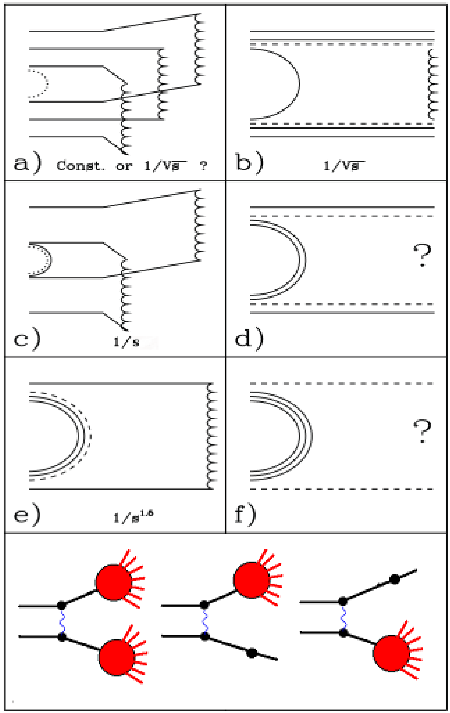
Fig. 41 Quark flow diagrams of \(\bar pp\)-interactions.
As usual, quarks and anti-quarks are shown by solid lines. Dashed lines present so-called string junctions. It is assumed that the gluon field in baryons has a non-trivial topology. This heterogeneity is called a “string junction”. Quark-gluon strings produced in the reaction are shown by wavy lines.
The diagram of Fig. 41(a) represents a process with a string junction annihilation and the creation of three strings. Diagram Fig. 41(b) describes quark-antiquark annihilation and string creation between the di-quark and anti-di-quark. Quark-anti-quark and string junction annihilation is shown in Fig. 41(c). Finally, one string is created in the process of Fig. 41(e). Hadrons appear at the fragmentation of the strings in the same way that they appear in \(e^+e^-\)-annihilation. One can assume that excited strings with complicated gluonic field configurations are created in processes Fig. 41(d) and Fig. 41(f). If the collision energy is sufficiently small, glueballs can be formed in the process Fig. 41(f). Mesons with constituent gluons or with hidden baryon number can be created in process Fig. 41(f). Of course the standard FTF processes shown in the bottom of the figure are also allowed.
In the simplest approach it is assumed that the energy dependence of the cross sections of these processes vary inversely with a power of \(s\) as depicted in Fig. 41. Here \(s\) is the center-of-mass energy squared. This is dictated by the reggeon phenomenology. Calculating the cross sections of binary reactions is a rather complicated procedure (see [Kaidalov_Bin]) because there can be interactions in the initial and final states. These interactions reflect also on cross sections of other reactions [Uzhinsky_GaloyanPbarP].
The annihilation cross section is given as:
where \(X_i\) are yields of the diagrams of Fig. 41. All cross sections are given in mb.
\(\bar pp\) |
\(\bar pn\) |
\(\bar np\) |
\(\bar nn\) |
\(\bar \Lambda p\) |
\(\bar \Lambda n\) |
\(\bar \Sigma^-p\) |
\(\bar \Sigma^-n\) |
\(\bar \Sigma^0p\) |
\(\bar \Sigma^0n\) |
\(\bar \Sigma^+p\) |
\(\bar \Sigma^+n\) |
|
B |
5 |
4 |
4 |
5 |
3 |
3 |
2 |
4 |
3 |
3 |
4 |
2 |
C |
5 |
4 |
4 |
5 |
3 |
3 |
2 |
4 |
3 |
3 |
4 |
2 |
D |
6 |
4 |
4 |
6 |
3 |
3 |
2 |
2 |
2 |
2 |
2 |
0 |
\(\bar \Xi^-p\) |
\(\bar \Xi^-n\) |
\(\bar \Xi^0p\) |
\(\bar \Xi^0n\) |
\(\bar \Omega^-p\) |
\(\bar \Omega^-n\) |
|
B |
1 |
2 |
2 |
1 |
0 |
0 |
C |
1 |
2 |
2 |
1 |
0 |
0 |
D |
0 |
0 |
0 |
0 |
0 |
0 |
The coefficients B, C and D are pure combinatorial coefficients calculated on the assumption that the same conditions apply to all quarks and anti-quarks. For example, in \(\bar pp\) interactions there are five possibilities to annihilate a quark and an anti-quark, and six possibilities to annihilate two quarks and two anti-quarks. Thus, \(B=C=5\) and \(D=6\). Note that final state particles in the process of Fig. 41(b) can coincide with initial state particles. Thus the true elastic cross section is not given by the experimental cross section.
At \(P_{lab} < 40 \mathrm{MeV/c}\) anti-proton-nucleon cross sections are:
All cross sections are given in [mb].
At \(P_{lab} < 40\) MeV/c, \(\sigma_b\) must be equal 0 for
\(\bar pp\)-interactions because the process
\(\bar pp \rightarrow \bar nn\) is impossible at these energies.
It is not so for \(\bar nn\) interactions because the process
\(\bar nn \rightarrow \bar pp\) can take place. In the case
\(\bar np\) interactions, the process “b” will lead to elastic
scattering which is not considered. The parameterizations are presented in the
lines 236 — 357. Their changes influence on
\(\bar pp\) channel cross sections. Thus, the changes must be done with caution.
To complete the cross section calculations, \(\sigma_{FTF}\)
responsible for processes presented in bottom row of Fig. 41
is determined (line 346) as:
where \(s_{th}\) is the threshold energy of meson production \(\left(m_{pr} + m_{tr} + m_\pi + 80 \right)^2\) [MeV].
After that, after line 478, needed quantities are stored in G4FTFParameters class:
SetTotalCrossSection( Xtotal );
SetElastisCrossSection( Xelastic );
SetInelasticCrossSection( Xtotal - Xelastic );

SetProbabilityOfElasticScatt( Xtotal, Xelastic );
SetRadiusOfHNinteractions2( Xtotal/pi/10.0 );

SetProbabilityOfAnnihilation( Xannihilation / (Xtotal - Xelastic) );

SetSlope( Xtotal*Xtotal/16.0/pi/Xelastic/0.3894 );
SetGamma0( GetSlope()*Xtotal/10.0/2.0/pi );

// Parameters of elastic scattering
// Gaussian parametrization of elastic scattering amplitude assumed
SetAvaragePt2ofElasticScattering( 1.0/( Xtotal*Xtotal/16.0/pi/Xelastic/0.3894 )

G4double Xinel = Xtotal - Xelastic;
Cross sections of elementary processes
The Fritiof model [Fritiof1], [Fritiof2] assumes that all hadron-hadron interactions are binary reactions, \(h_1 + h_2 \rightarrow h_1^\prime + h_2^\prime\) where \(h_1^\prime\) and \(h_2^\prime\) are excited states of the hadrons with discrete or continuous mass spectra (see Fig. 42). If one of the final hadrons is in its ground state (\(h_1 +h_2 \rightarrow h_1 + h_2^\prime\)) the reaction is called “single diffraction dissociation”, and if neither hadron is in its ground state it is called a “non-diffractive” interaction.
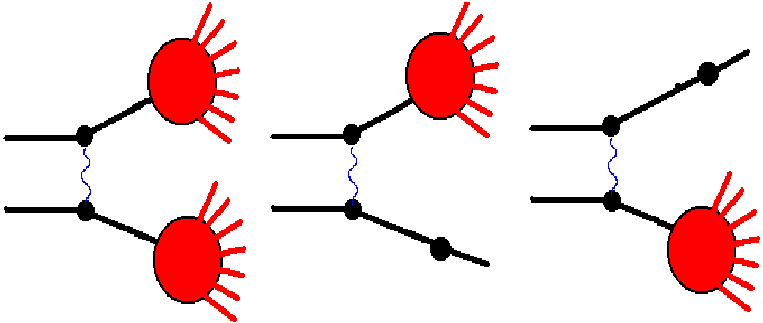
Fig. 42 Non-diffractive and diffractive interactions considered in the Fritiof model.
The excited hadrons are considered as QCD-strings, and the corresponding LUND-string fragmentation model is applied in order to simulate their decays.
The key ingredient of the Fritiof model is the sampling of the string masses. In general, the set of final states for the interactions can be represented by Fig. 43, where samples of possible string masses are shown. There is a point corresponding to elastic scattering, a group of points which represents final states of binary hadron-hadron interactions, lines corresponding to the diffractive interactions, and various intermediate regions. The region populated with the red points is responsible for the non-diffractive interactions. In the model, the mass sampling threshold is set equal to the ground state hadron masses, but in principle the threshold can be lower than these masses. The string masses are sampled in the triangular region restricted by the diagonal line corresponding to the kinematical limit \(M_1 + M_2 = E_{cms}\) where \(M_1\) and \(M_2\) are the masses of the \(h_1^\prime\) and \(h_ 2^\prime\) hadrons, and also of the threshold lines. If a point is below the string mass threshold, it is shifted to the nearest diffraction line.

Fig. 43 Diagram of the final states of hadron-hadron interactions.
Unlike the original Fritiof model, the final state diagram of the current model is complicated, which leads to a non-straightforward mass sampling algorithm. This will be considered below. The original model had no points corresponding to elastic scattering or to the binary final states. As it was known at the time, the mass of an object produced by diffraction dissociation, \(M_x\), for example from the reaction \(p+p \rightarrow p + X\), is distributed as \(dM_x / M_x \propto dM_x^2 / M_x^2\), so it was natural to assume that the object mass distributions in all inelastic interactions obey the same law. This can be re-written using the light-cone momentum variables, \(P^+\) or \(P^-\),
where \(E\) is the energy of a particle, and \(p_z\) is its longitudinal momentum along the collision axis. At large energy and positive \(p_z\) , \(P^- \simeq (M^2 + P_T^2) / 2p_z\). At negative \(p_z\), \(P^+ \simeq (M^2 + P_T^2) / 2|p_z|\). Usually, the transferred transverse momentum, \(P_T\), is small and can be neglected. Thus, it was assumed that \(P^-\) and \(P^+\) of a projectile and target associated hadron, respectively, are distributed as
A gaussian distribution was used to sample \(P_T\).
In the case of hadron-nucleus or nucleus-nucleus interactions it was assumed that the created objects can interact further with other nuclear nucleons and create new objects. Assuming equal masses of the objects, the multiplicity of particles produced in these interactions will be proportional to the number of participating nuclear nucleons, or to the multiplicity of intra-nuclear collisions. Due to this, the multiplicity of particles produced in hadron-nucleus or nucleus-nucleus interactions is larger than that in hadron-hadron ones. The probabilities of multiple intra-nuclear collisions were sampled with the help of a simplified Glauber model. Cascading of secondary particles was not considered.
Because the Fermi motion of nuclear nucleons was simulated in a simple manner, the original Fritiof model could not work at \(P_{lab} <\) 10 – 20 GeV/c.
It was assumed in the model that the created objects are quark-gluon strings with constituent quarks at their ends originating from the primary colliding hadrons. Thus, the LUND-string fragmentation model was applied for a simulation of the object decays. It was assumed also that the strings with sufficiently large masses have “kinks” – additional radiated gluons. This is very important for a correct reproduction of particle multiplicities in the interactions.
All of the above assumptions were reconsidered in the implementation of the Geant4 Fritiof model, and new features were added. These will be presented below.

Fig. 44 Quark flow diagrams of \(\pi N\) interactions.
The original Fritiof model contains only the pomeron exchange process shown in Fig. 44(d). It would be useful to extend the model by adding the exchange processes shown in Fig. 44(b) and Fig. 44(c), and the annihilation process of Fig. 44(a). This could probably be done by introducing a restricted set of mesonic and baryonic resonances and a corresponding set of parameters. This procedure was employed in the binary cascade model of Geant4 (BIC) [BIC] and in the Ultra-Relativistic-Quantum-Molecular-Dynamic model (UrQMD) [UrQMD1], [UrQMD2]. However, it is complicated to use this solution for the simulation of hadron-nucleus and nucleus-nucleus interactions. The problem is that one has to consider resonance propagation in the nuclear medium and take into account their possible decays which enormously increases computing time. Thus, in the current version of the FTF model only quark exchange processes have been added to account for meson and baryon interactions with nucleons, without considering resonance propagation and decay. This is a reasonable hypothesis at sufficiently high energies.
For each projectile hadrons the following probabilities are set up:
Probability of quark exchange process without excitation of participants (Fig. 44(b)); (Proc# 0)
Probability of quark exchange process with excitation of participants (Fig. 44(c)); (Proc# 1)
Probability of projectile diffraction dissociation; (Proc# 2)
Probability of target diffraction dissociation. (Proc# 3)
All these probabilities have the same functional form:
where \(y\) is the projectile rapidity in the target rest frame.
For each projectile hadron and for each possible process,
SetParams method is called for setting up the parameters
\(A_1\) , \(B_1\) , \(A_2\) , \(B_2\), \(A_3\) .
For projectile baryons, this is implemented in
lines 524 — 542 .
//         Proc#  A1        B1            A2       B2    A3  Atop  Ymin
SetParams(   0, 13.71,     1.75,          -214.5, 4.25, 0.0, 0.5 , 1.1 );
SetParams(   1, 25.0 ,     1.0 ,          -50.34, 1.5 , 0.0, 0.0 , 1.4 );
if ( Xinel > 0.0 ) {
  SetParams( 2, 6.0/Xinel, 0.0 ,-6.0/Xinel*16.28, 3.0 , 0.0, 0.0 , 0.93 );
  SetParams( 3, 6.0/Xinel, 0.0 ,-6.0/Xinel*16.28, 3.0 , 0.0, 0.0 , 0.93 );
  SetParams( 4, 1.0 ,      0.0 ,           -2.01, 0.5 , 0.0, 0.0 , 1.4 );
} else {
  SetParams( 2, 0.0,       0.0 ,            0.0 , 0.0 , 0.0, 0.0 , 0.0 );
  SetParams( 3, 0.0,       0.0 ,            0.0 , 0.0 , 0.0, 0.0 , 0.0 );
  SetParams( 4, 0.0,       0.0 ,            0.0 , 0.0 , 0.0, 0.0 , 0.0 );
}
if ( AbsProjectileBaryonNumber > 1  ||  NumberOfTargetNucleons > 1 ) {
  SetParams( 2, 0.0,       0.0 ,            0.0 , 0.0 , 0.0, 0.0 , -100.0 );
  //SetParams( 3, 0.0,       0.0 ,            0.0 , 0.0 , 0.0, 0.0 , -100.0 );
}
Proc# are the quark exchange without participant excitation (0), the quark
exchange with participant excitation (1), projectile diffraction (2),
target diffraction (3). The probability of the quark exchange with
participant excitation has an additional multiplier ( Proc#=4).
Probability of non-diffractive interactions is
\(P_{nd} =1-P_0 -P_1 *P_4 - P_2 -P_3\).
If the target is a nucleus, \(P_2\) is set to zero, because it is not clear
up to now how to deal with projectile diffraction on nuclei. This is implemented in
lines 537 — 542.
Due to quark exchange without participant excitation one or two final
particles can be in \(\Delta\) resonance state. The probability of this is
set up in the line 543: SetDeltaProbAtQuarkExchange( 0.0 );.
Next lines: 544 — 548, set up a probability of the same quark’s exchange
between interacting hadrons.
if ( NumberOfTargetNucleons > 26 ) {
  SetProbOfSameQuarkExchange( 1.0);
} else {
  SetProbOfSameQuarkExchange( 0.0 );
}
An exchange with the same quark in baryon-baryon interactions is expected to be suppressed at low energies. It cannot be so at high energies. The energy dependence of the parameter and its influence on final results is not yet well studied.
Using the probability of the same quark’s exchange, one can obtain the yield to the elastic scattering cross section. Thus, self-consistent change of the parametrization of the elastic cross section can be needed.
Parameters of participating hadron excitations
In the lines 549 — 555 the parameters of the excitations are set up.:
SetProjMinDiffMass( 1.16 );     // GeV
SetProjMinNonDiffMass( 1.16 );  // GeV
SetTarMinDiffMass( 1.16 );      // GeV
SetTarMinNonDiffMass( 1.16 );   // GeV
SetAveragePt2( 0.15 );          // GeV^2
SetProbLogDistrPrD( 0.3 );
SetProbLogDistr( 0.3 );
The first line determines the string mass sampling threshold (see Fig. 43) in diffractive processes. For baryons, it is \(1160=m_N +m_\pi + 80 [\mathrm{MeV}]\). The second line is the analogous threshold for non-diffractive processes. The third and fourth lines set up analogous values for the target nucleon. A change of the parameters will lead to a change of the threshold behaviour of mass distribution in the reaction \(p+p \rightarrow p+X\).
An average transverse momentum in the excitation is set up in the fifth line. Its change will change behaviour of particle distributions at large \(x_F\). For pure diffractive processes the average is determined in G4ElasticHNScattering as for the elastic scattering. It is known that the slope of \(p_T\) distribution in diffraction processes (\(p+p \rightarrow p+X\), for example) depends on the produced mass of system \(X\). Here an improvement can be introduced.
Parameters set up in lines sixth and seventh are very important for a correct description of produced particles multiplicity in non-diffractive interactions. It is assumed in the code that mass distribution of strings produced in non-diffractive interactions has the form:
\(\alpha\) can be different for projectile and target hadrons. The sixth line sets up the parameter for a projectile hadron, and the seventh line for a target hadron. A variation of the parameters can have an essential influence on multiplicity of produced particles.
The analogous lines are presented for each type of projectile hadron.
Nuclear destruction parameters
The nuclear destruction parameters are set up in the
lines 672 — 717 . For a meson projectile they are:
if ( ProjectileabsPDGcode < 1000 ) {  // Meson projectile
  SetMaxNumberOfCollisions( Plab, 2.0 );
  SetCofNuclearDestruction( 1.0*
          G4Exp( 4.0*(Ylab - 2.1) )/( 1.0 + G4Exp( 4.0*(Ylab - 2.1) ) ) );
  SetR2ofNuclearDestruction( 1.5*fermi*fermi );
  SetDofNuclearDestruction( 0.3 );
  SetPt2ofNuclearDestruction( ( 0.035 + 0.04*G4Exp( 4.0*(Ylab - 2.5) )/
                                        ( 1.0 + G4Exp( 4.0*(Ylab - 2.5) ) ) )*GeV*GeV );
  SetMaxPt2ofNuclearDestruction( 1.0*GeV*GeV );
  SetExcitationEnergyPerWoundedNucleon( 40.0*MeV );
}
The second line introduces the maximum number of intra-nuclear collisions used as a correction of the Abramovski-Gribov-Kancheli (AGK) cutting rules (see Geant4 Physics Reference Manual).
The FTF model uses the reggeon cascading for simulation of fast nucleon production in hadron-nucleus interactions. As known, the Glauber approximation used in the Fritiof model and in the other string models does not provide enough amount of intra-nuclear collisions for a correct description of nuclear destruction. Additional cascading in nuclei is therefore needed. The usage of standard cascade for secondary particle interactions would lead to a too large multiplicity of produced particles. Thus, in Ref. [RTIM1] and [RTIM2] it was proposed to use reggeon cascading in the impact parameter space. For its description it is needed to determine the probability to involve a nuclear nucleons into the “cascade”. It is obvious that the probability depends on the difference of impact coordinates of new and previous involved nucleons. Looking at the yield of reggeon enhanced diagrams, the functional form of the probability was chosen as:
where \(\vec{s}_i\) and \(\vec{s}_j\) are projections of the radii of i-th and j-th nucleons on the impact parameter plane.
The “cascade” is initiated by primary involved nucleons. These nucleons are determined with the help of the Glauber approach. All involved nucleons are ejected from nuclei. The cascade looks like that: a projectile particle interacts with some intra-nuclear nucleons. These nucleons are called “wounded” or “participating” nucleons. The nucleons initiate the cascade. A wounded nucleon can involve a spectator nucleon into the cascade with the probability \(P\). The latter one can involve another nucleon. The second nucleon can involve a third one and so on. This algorithm is implemented in the FTF model.
We have tuned \(C_nd\) using the HARP-CDP data on proton production in the \(p+Cu\) interactions [HARP_CDP]. According to our estimations,
where \(y\) is the projectile rapidity. The value 2.1, standing in the exponents, corresponds to \(P_{lab} \sim 4 \mathrm{GeV/c}\), which is the middle of the transition region between low and high energies.
The formula is implemented in the third and fourth lines. Its parameters, of course, can be changed to improve description of the fast nucleon production in the target fragmentation region.
The parameters \(C_nd\) and \(R_c\) are strongly correlated. To avoid this, \(R_c\) was fixed (fifth line).
Momentum distribution of wounded and involved nucleons of a nucleus is sampled according to the distribution:
where \(M_N\) is the multiplicity of involved nucleons, \(x\) is the light-cone momentum fraction carried by the nucleon relative to light-cone momentum of the nucleus, \(d\) is the dispersion parameter responsible for a spread of the momentum distribution, \(\vec{P}_T\) is the transverse momentum, \(\langle P_T^2 \rangle\) is the average \(P_T\) squared. \(d\) is setting up in the sixth line. Possible value of \(d\) can be 0.1 — 0.4.
\(\langle P_T^2 \rangle\) is determined in the lines 7, 8. Again, an expression
giving asymptotically constant value is used:
\(\langle P_T^2 \rangle\) must be small at low energies, and grows up as energy increase. All coefficients in the expression can be tuned. Their preliminary values were determined from the HARP-CDP experimental data.
The last, tenth line sets up the yield of an involved nucleon to the
excitation energy of a nuclear residual in MeV. The commented
lines 719 — 752 are needed for testing purposes, for easily setting up of the
parameters.
Changing parameters of an existing model: Lund use-case
The main parameters of the Geant4 LUND string fragmentation model are in
the file G4LundStringFragmentation.cc located in
geant4/source/processes/hadronic/models/parton\_string/hadronization/src.
The main method of the class is FragmentString
which is called by the class G4ExcitedStringDecay.
The input parameter of the method is an object type G4ExcitedString.
At the beginning of this method it is checked that the string can
fragment (line 537, !IsFragmentable(&aString)).
If the mass of the string does not allow a two particles decay, then
the string is considered as a single hadron out of mass-shell. The
minimal mass of the string that can decay is determined in the method
SetMinimalStringMass (line 413).
If the string can fragment, the main routine starts to work –
Loop_toFragmentString
. The loop is working until it is decided to stop fragmentation of the
string in the method StopFragmenting (lines 643 — 655).
There are two important parameters in the method:
G4bool G4LundStringFragmentation::StopFragmenting(const G4FragmentingString * const string)
{
  SetMinimalStringMass(string);
  if (string->FourQuarkString())
  {
    return G4UniformRand() < G4Exp(-0.0005*(string->Mass() - MinimalStringMass));
  } else {
    return G4UniformRand() < G4Exp(-0.66e-6*(string->Mass()*string->Mass() -
                                             MinimalStringMass*MinimalStringMass));
  }
}
“0.0005” and “0.66e-6”. The first one is responsible for the energy dependence of cross sections of the processes: \(\bar p + p \rightarrow \bar q \bar q + qq \rightarrow h_1 + h_2\). The second one determines the energy dependence of cross sections for hadronic interactions at low energies.
If the fragmentation is not stopped, the code is trying to create a
hadron splitting the string (line 1033,
G4KineticTrack * Hadron=Splitup(currentString,newString)).
The method G4VLongitudinalStringDecay::Splitup
samples a side of the string decay: left or right string ends. Depending
on type of a quark on the decaying end, a quark splitting, or a di-quark
splitting is called. After them, a produced hadron momentum is
determined in the method SplitEandP.
The method QuarkSplitup is implemented in G4VLongitudinalStringDecay
class. There can be two possibilities:
\(q \rightarrow h(q \bar q^\prime) + q^\prime\) and
\(q \rightarrow B(q\ (qq)^\prime) + (\bar q \bar q)^\prime\).
A quark-antiquark pair is produced from the vacuum in the first case,
and a meson \(h\) appears. A di-quark-anti-diquark pair is produced
from the vacuum in the second case, and a baryon \(B\)
appears. The probability of the second case is given by the parameter
DiquarkSuppress inherited from the parent class
G4VLongitudinalStringDecay. It is reset in G4LundStringFragmentation.cc
(line 69, SetDiquarkSuppression(0.05)). The probability of the first case is
\(1-DiquarkSuppress\).
The pairs created in the first case can consist of light quarks
(\(u\bar u\) , \(d\bar d\)), or strange quarks (\(s\bar s\)).
The probability of the last possibility is
\(StrangeSuppress/(2+StrangeSuppress)\). The parameter StrangeSuppress
is set up in G4LundStringFragmentation.cc
(line 395, SetStrangenessSuppression(0.46)).
By increasing this parameter the strange meson production increases.
At creation of the diquark-anti-diquark pair, the flavors of both quarks are sampled independently. Thus, the probability to produce a strange baryon in central region is roughly proportional to StrangeSuppress.
The created meson can be a pseudo-scalar, or pseudo-vector one. The
probability of a pseudo-scalar meson creation (pspin_meson)
is set up in the parent class - G4VLongitudinalStringDecay (see
line 82 in G4VLongitudinalStringDecay.cc). The probability of a
pseudo-vector meson creation is 1-pspin_meson.
The created baryon can belong to triplet or octet multiplets. The
probability of the triplet state is given by the parameter
pspin_barion determined in the parent class G4VLongitudinalStringDecay
(line 85 of G4VLongitudinalStringDecay.cc). It is foreseen the
possibility to change pspin_barion in the
G4LundStringFragmentation.cc (line 176, //pspin_barion=0.75;).
Warning
It is not recommended to change pspin_meson and pspin_barion!
In the method G4LundStringFragmentation::DiQuarkSplitup two
possibilities are considered:
\(q_1q_2 \rightarrow h(q_1 \bar q^\prime) + q^\prime q_2\)
and
\(q_1q_2 \rightarrow B(q_1q_2 \ q^\prime) + \bar q^\prime\).
The probability of the first process is
regulated by the parameter DiquarkBreakProb. It is set up in
G4LundStringFragmentation.cc (line 67,
SetDiquarkBreakProbability(0.05)). This parameter is responsible for
the meson production in hadronic interactions at large values
\(|x_F|\) .
The StrangeSuppress parameter is changed for the second process (see
line 1487, StrangeSuppress=0.43).
After the creation of a hadron its momentum is determined in the method SplitEandP which has as input the type of the produced hadron and the string, and as input-output the residual string left after the hadron momentum sampling. At the beginning, only the quark content of the residual string is known. If the hadron mass plus a minimal mass of the residual string is larger than the mass of the initial string, then the sampling of the hadron is repeated as described above. If it is not so, an attempt to determine the hadron momentum is undertaken.
First of all, the transverse momentum of the hadron is sampled. The transverse momentum distribution is given by the formula:
If the sum of the transverse mass of the hadron and the transverse mass
of the residual string is larger than the initial string mass, then the
attempt is repeated. If it is not so, the longitudinal momentum of the
hadron is sampled with the help of the GetLightConeZ method
(lines 928 — 981).
The LUND string fragmentation functions is implemented in GetLightConeZ. The method gives light-cone-momentum fraction of the initial string carried away by the hadron.
\(a=0.7 [\mathrm{GeV}^{-2}]\) for quark fragmentation,
and for a production of a meson by a di-quark (line 941).
The di-quark fragmentation function is assumed to be a flat distribution between
\(z_{min}\) and \(z_{max}\) ( line 978).
When the fragmentation of a string is stopped, SplitLast
method ( lines 658 — 753) is called. Depending of the quark content of the string,
Diquark_AntiDiquark_belowThreshold_lastSplitting, or
Diquark_AntiDiquark_aboveThreshold_lastSplitting, or
Quark_AntiQuark_lastSplitting, or
Quark_Diquark_lastSplitting
is called. The methods determine the types of the two last produced
particles. After that, 4-momentum of the particles are calculated
(Sample4Momentum , line 744). If at least one of the two final
hadrons is a baryon, an isotropic decay is simulated with a probability
ProbIsotropy (line 764),
The power 4 and functional form of the dependence can be tuned. It can reflect on angular distributions of baryons in annihilation processes, or in low energy interactions.
If anisotropic decay happens, then the \(p_T\) of final hadrons is simulated as before.
For the sampling of the two final hadrons special arrays are introduced in the
lines 81 — 375.
- 1
The same can be achieved with template specialisations with slightly improved CPU performance but at the cost of significantly more complex designs and, with present compilers, significantly reduced portability.