Gamma Conversion into \(\mu ^+\mu ^-\) Pair
The class G4GammaConversionToMuons simulates the process of gamma conversion into muon pairs. Given the photon energy and \(Z\) and \(A\) of the material in which the photon converts, the probability for the conversions to take place is calculated according to a parameterized total cross section. Next, the sharing of the photon energy between the \(\mu^+\) and \(\mu^-\) is determined. Finally, the directions of the muons are generated. Details of the implementation are given below and can be also found in [BKK02].
Cross Section and Energy Sharing
Muon pair production on atomic electrons, \(\gamma+e\to e+\mu^+ +\mu^-\), has a threshold of \(2m_\mu(m_\mu+m_e)/m_e\approx 43.9\;{\rm GeV}\) . Up to several hundred GeV this process has a much lower cross section than the corresponding process on the nucleus. At higher energies, the cross section on atomic electrons represents a correction of \(\sim 1/Z\) to the total cross section.
For the approximately elastic scattering considered here, momentum, but no energy, is transferred to the nucleon. The photon energy is fully shared by the two muons according to
or in terms of energy fractions
The differential cross section for electromagnetic pair creation of muons in terms of the energy fractions of the muons is
where \(Z\) is the charge of the nucleus, \(r_c\) is the classical radius of the particles which are pair produced (here muons) and
where
For hydrogen, \(B=202.4\) and \(D_n=1.49\). For all other nuclei, \(B=183\) and \(D_n=1.54 A^{0.27}\).
These formulae are obtained from the differential cross section for muon bremsstrahlung [KKP95] by means of crossing relations. The formulae take into account the screening of the field of the nucleus by the atomic electrons in the Thomas-Fermi model, as well as the finite size of the nucleus, which is essential for the problem under consideration. The above parameterization gives good results for \(E_\gamma \gg m_\mu\). The fact that it is approximate close to threshold is of little practical importance. Close to threshold, the cross section is small and the few low energy muons produced will not travel very far. The cross section calculated from Eq.(15) is positive for \(E_\gamma > 4 m_\mu\) and
except for very asymmetric pair-production, close to threshold, which can easily be taken care of by explicitly setting \(\sigma = 0\) whenever \(\sigma < 0\).
Note that the differential cross section is symmetric in \(x_+\) and \(x_-\) and that
where \(x\) stands for either \(x_+\) or \(x_-\). By defining a constant
the differential cross section Eq.(15) can be rewritten as a normalized and symmetric as function of \(x\):
This is shown in Fig. 3 for several elements and a wide range of photon energies. The asymptotic differential cross section for \(E_\gamma \rightarrow \infty\)
is also shown.
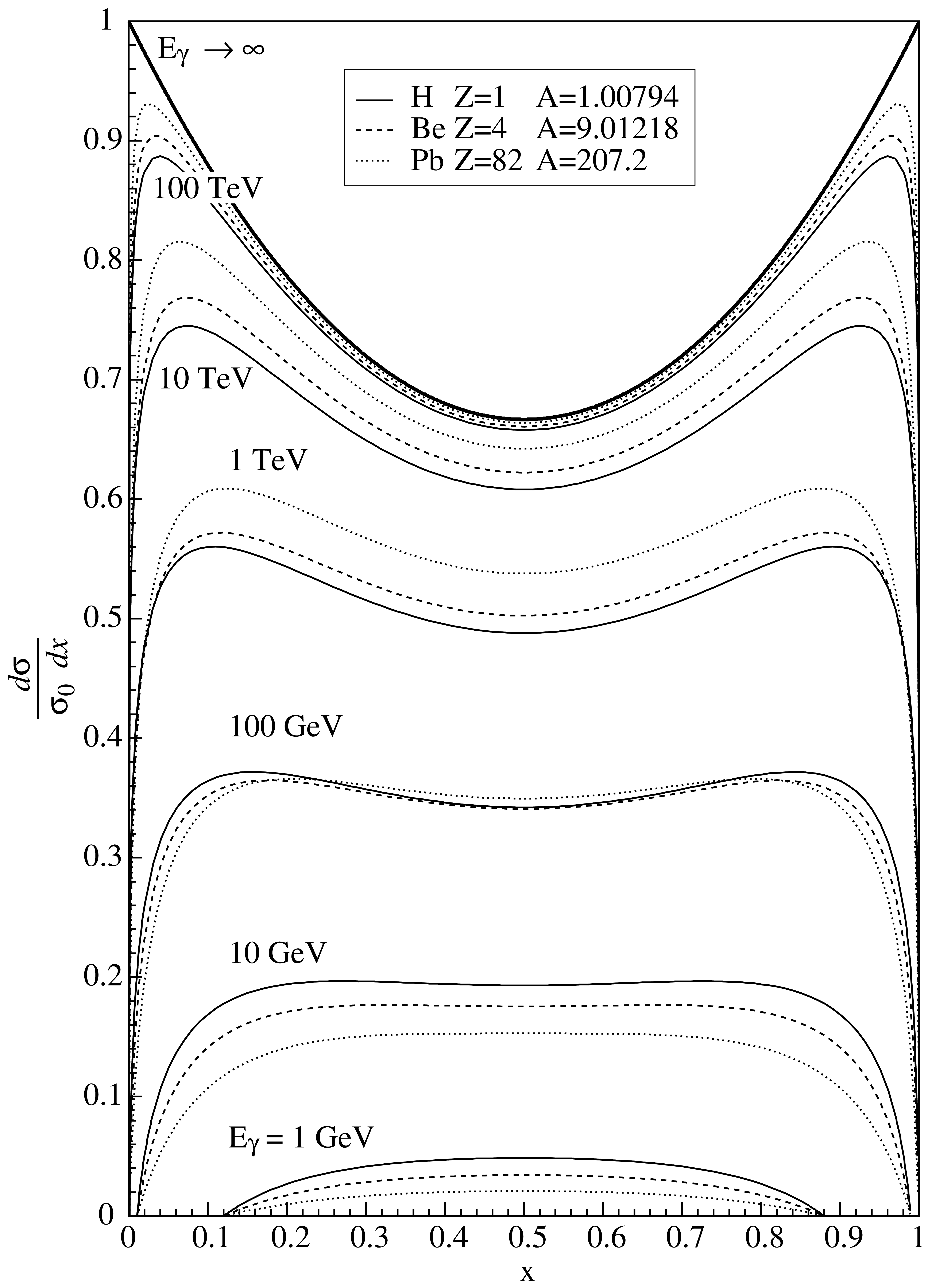
Fig. 3 Normalized differential cross section for pair production as a function of \(x\), the energy fraction of the photon energy carried by one of the leptons in the pair. The function is shown for three different elements, hydrogen, beryllium and lead, and for a wide range of photon energies.
Parameterization of the Total Cross Section
The total cross section is obtained by integration of the differential cross section Eq.(15), that is
\(W\) is a function of (\(x_+, E_\gamma\)) and (\(Z, A\)) of the element (see Eq.(16)). Numerical values of \(W\) are given in Table 7.
\(E_\gamma\) [GeV] |
W for H |
W for Be |
W for Cu |
W for Pb |
1 |
2.11 |
1.594 |
1.3505 |
5.212 |
10 |
19.4 |
10.85 |
6.803 |
43.53 |
100 |
191.5 |
102.3 |
60.10 |
332.7 |
1000 |
1803 |
919.3 |
493.3 |
1476.1 |
10000 |
11427 |
4671 |
1824 |
1028.1 |
\(\infty\) |
28087 |
8549 |
2607 |
1339.8 |
Values of the total cross section obtained by numerical integration are listed in Table 8 for four different elements. Units are in \(\mu{\rm barn}\,\), where \(1\,\mu{\rm barn} = 10^{-34}\,{\rm m}^2\,\).
\(E_\gamma\) [GeV] |
\(\sigma_{\rm tot}\), H [\(\mu{\rm barn}\,\)] |
\(\sigma_{\rm tot}\), Be [\(\mu{\rm barn}\,\)] |
\(\sigma_{\rm tot}\), Cu [\(\mu{\rm barn}\,\)] |
\(\sigma_{\rm tot}\), Pb [\(\mu{\rm barn}\,\)] |
1 |
0.01559 |
0.1515 |
5.047 |
30.22 |
10 |
0.09720 |
1.209 |
49.56 |
334.6 |
100 |
0.1921 |
2.660 |
121.7 |
886.4 |
1000 |
0.2873 |
4.155 |
197.6 |
1476 |
10000 |
0.3715 |
5.392 |
253.7 |
1880 |
\(\infty\) |
0.4319 |
6.108 |
279.0 |
2042 |
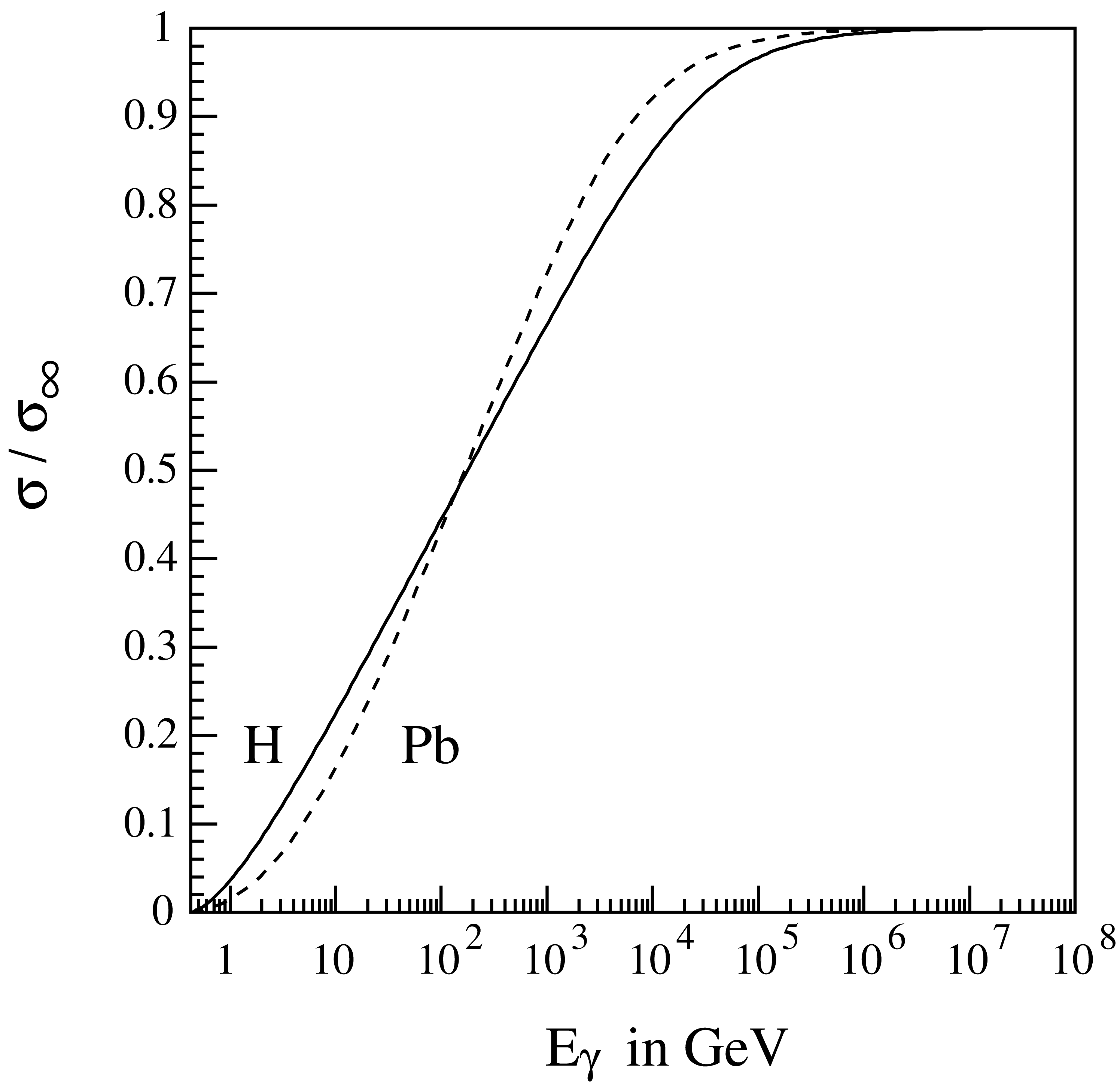
Fig. 4 Total cross section for the Bethe-Heitler process \(\gamma \rightarrow \mu^+\mu^-\) as a function of the photon energy \(E_\gamma\) in hydrogen and lead, normalized to the asymptotic cross section \(\sigma_\infty\).
Well above threshold, the total cross section rises about linearly in \(\log(E_\gamma)\) with the slope
until it saturates due to screening at \(\sigma_\infty\). Fig. 4 shows the normalized cross section where
Numerical values of \(W_M\) are listed in Table 11.
Element |
\(W_M\) [1/GeV] |
H |
0.963169 |
Be |
0.514712 |
Cu |
0.303763 |
Pb |
0.220771 |
The total cross section can be parameterized as
with
and
The threshold behavior in the cross section was found to be well approximated by \(t = 1.479 + 0.00799 D_n \) and the saturation by \(s = -0.88 \). The agreement at lower energies is improved using an empirical correction factor, applied to the slope \(W_M\), of the form
where
A comparison of the parameterized cross section with the numerical integration of the exact cross section shows that the accuracy of the parametrization is better than 2%, as seen in Fig. 5.
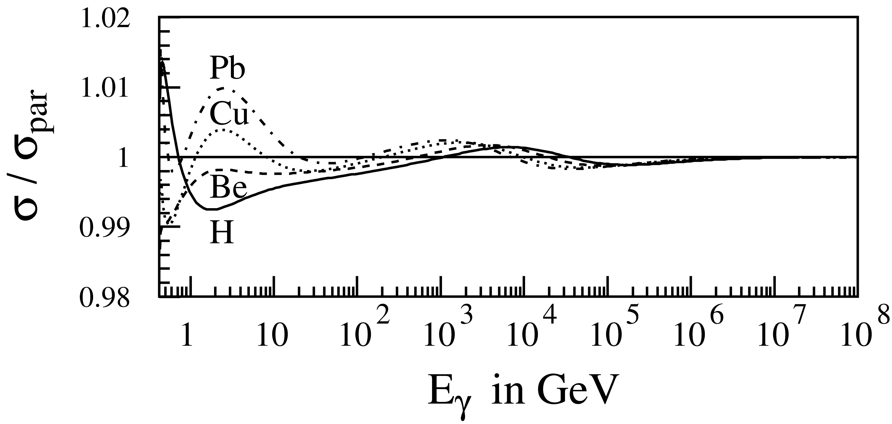
Fig. 5 Ratio of numerically integrated and parametrized total cross sections as a function of \(E_\gamma\) for hydrogen, beryllium, copper and lead.
Multi-differential Cross Section and Angular Variables
The angular distributions are based on the multi-differential cross section for lepton pair production in the field of the Coulomb center
Here
where
\(q^2\) is the square of the momentum \({\bf q}\) transferred to the target and \(q_{\parallel}^2\) and \(q_{\perp}^2\) are the squares of the components of the vector \({\bf q}\), which are parallel and perpendicular to the initial photon momentum, respectively. The minimum momentum transfer is \(q_{\min}=m_\mu^2/(2E_\gamma \, x_+x_-)\). The muon vectors have the components
where \(p_{\pm}=\sqrt{E_{\pm}^2-m_\mu^2}\). The initial photon direction is taken as the \(z\)-axis. The cross section of Eq.(21) does not depend on \(\varphi_0\). Because of azimuthal symmetry, \(\varphi_0\) can simply be sampled at random in the interval \((0,\,2\,\pi)\).
Eq.(21) is too complicated for efficient Monte Carlo generation. To simplify, the cross section is rewritten to be symmetric in \(u_+\), \(u_-\) using a new variable \(u\) and small parameters \(\xi,\beta\), where \(u_\pm=u \pm \xi/2\) and \(\beta = u \,\varphi\). When higher powers in small parameters are dropped, the differential cross section in terms of \(u,\xi,\beta\) becomes
where, in this approximation,
For Monte Carlo generation, it is convenient to replace (\(\xi,\beta\)) by the polar coordinates (\(\rho,\psi\)) with \(\xi=\rho\,\cos\psi\) and \(\beta=\rho\,\sin\psi\). Integrating Eq.(25) over \(\psi\) and using symbolically \(du^2\) where \(du^2 = 2 u \, du\) yields
Integration with logarithmic accuracy over \(\rho\) gives
Within the logarithmic accuracy, \(\log(m_\mu/q_{\parallel})\) can be replaced by \(\log(m_\mu/q_{\min})\), so that
Making the substitution \(u^2 = 1/t -1\), \(du^2 = -dt \, / t^2\) gives
Atomic screening and the finite nuclear radius may be taken into account by multiplying the differential cross section determined by Eq.(25) with the factor
where \(F_a\) and \(F_n\) are atomic and nuclear form factors. Please note that after integrating Eq.(26) over \(\rho\), the \(q\)-dependence is lost.
Procedure for the Generation of \(\mu ^+\mu ^-\) Pairs
Given the photon energy \(E_\gamma\) and \(Z\) and \(A\) of the material in which the \(\gamma\) converts, the probability for the conversions to take place is calculated according to the parametrized total cross section Eq.(20). The next step, determining how the photon energy is shared between the \(\mu^+\) and \(\mu^-\), is done by generating \(x_+\) according to Eq.(15). The directions of the muons are then generated via the auxilliary variables \(t,\,\rho,\,\psi\). In more detail, the final state is generated by the following five steps, in which \(R_{1,2,3,4,...}\) are random numbers with a flat distribution in the interval [0,1]. The generation proceeds as follows.
Sampling of the positive muon energy \(E_\mu^+ = x_+ \, E_\gamma\). This is done using the rejection technique. \(x_+\) is first sampled from a flat distribution within kinematic limits using
\[x_+ = x_{\rm min} + R_1 (x_{\rm max} - x_{\rm min})\]and then brought to the shape of Eq.(15) by keeping all \(x_+\) which satisfy
\[\left(1-\frac43\,x_+x_-\right)\frac{\log(W)}{\log(W_{\rm max})} < R_2 \,.\]Here \(W_{\rm max}= W(x_+=1/2)\) is the maximum value of \(W\), obtained for symmetric pair production at \(x_+=1/2\). About 60% of the events are kept in this step. Results of a Monte Carlo generation of \(x_+\) are illustrated in Fig. 6. The shape of the histograms agrees with the differential cross section illustrated in Fig. 3.
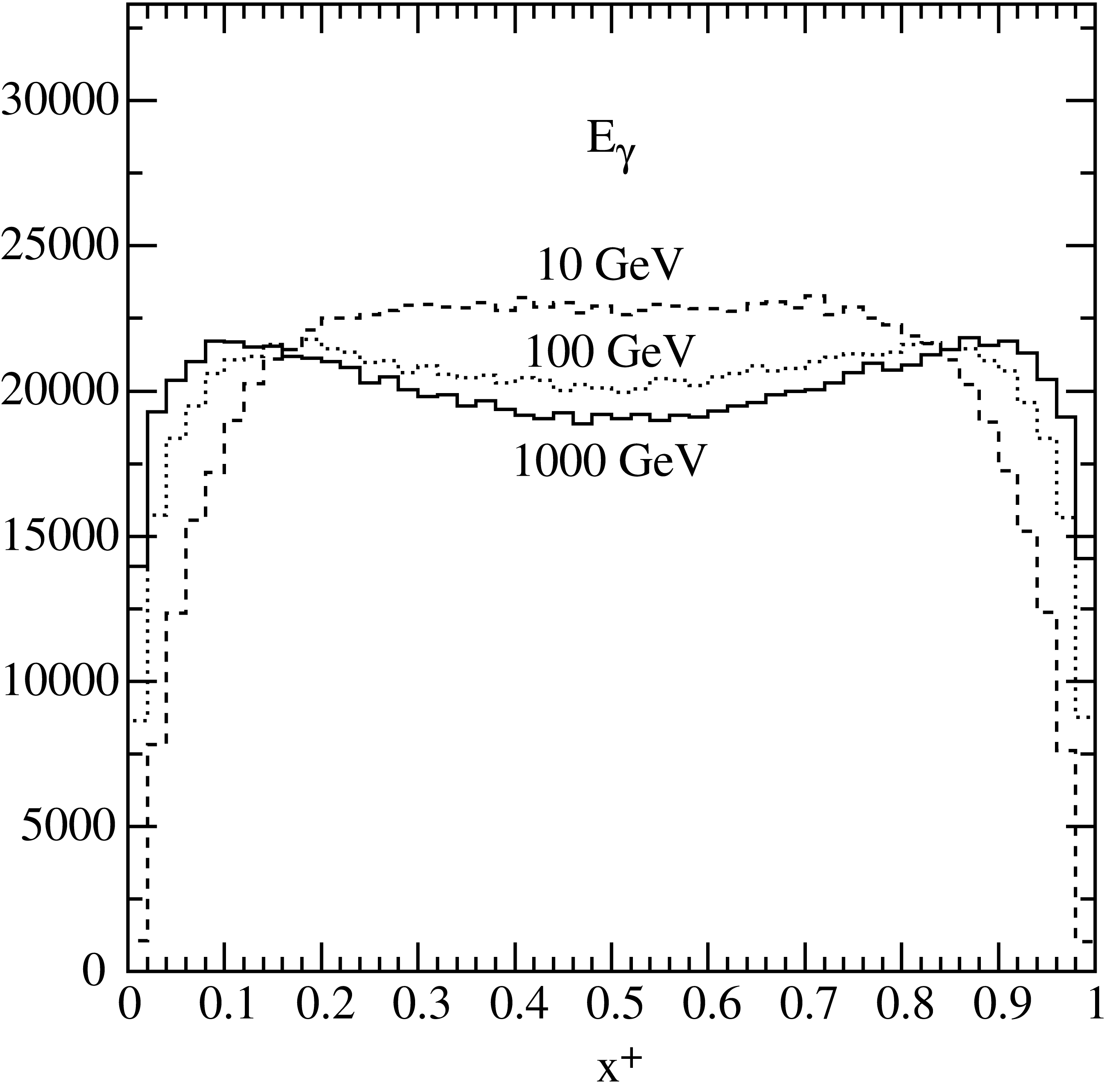
Fig. 6 Histogram of generated \(x_+\) distributions for beryllium at three different photon energies. The total number of entries at each energy is \(10^6\).
Generate \(t ( = \frac{1}{\gamma^2 \theta^2 + 1} )\) . The distribution in \(t\) is obtained from Eq.(27) as
\[f_1(t)\,dt=\frac{1-2\,x_+x_{-}+4\,x_+x_{-t}\,(1-t)} {1+C_1/t^2}\,dt\,,\quad 0<t\le 1\,.\]with form factors taken into account by
\[C_1= \frac{(0.35\,A^{0.27})^2}{x_+x_-\,E_\gamma/m_\mu }\,.\]In the interval considered, the function \(f_1(t)\) will always be bounded from above by
\[\max [f_1(t)]=\frac{1-x_+x_{-}}{1+C_1}\;.\,\]For small \(x_+\) and large \(E_{\gamma}\), \(f_1(t)\) approaches unity, as shown in Fig. 7.
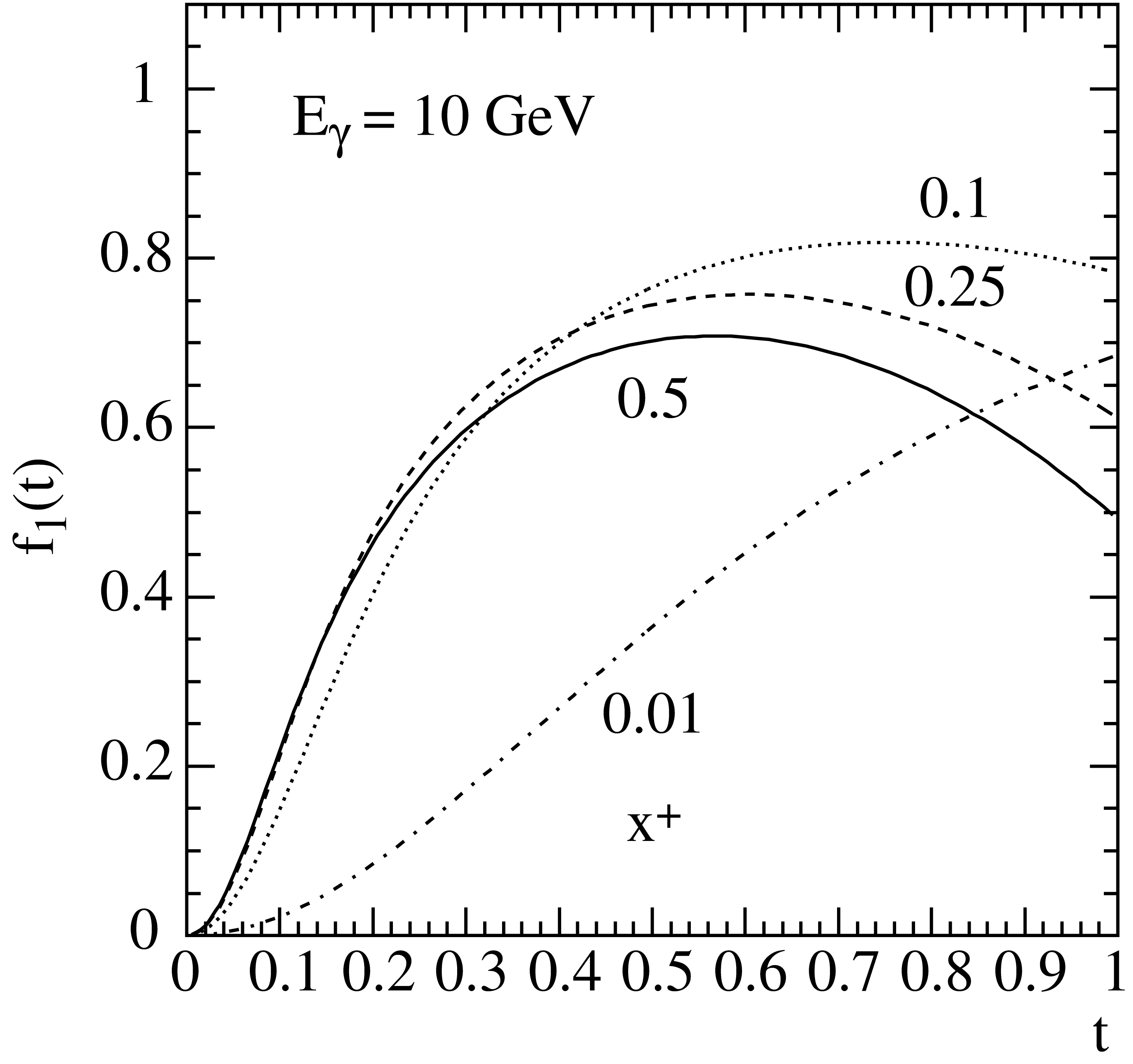
Fig. 7 The function \(f_1(t)\) at \(E_{\gamma} = 10\,{\rm GeV}\) in beryllium for different values of \(x_+\).
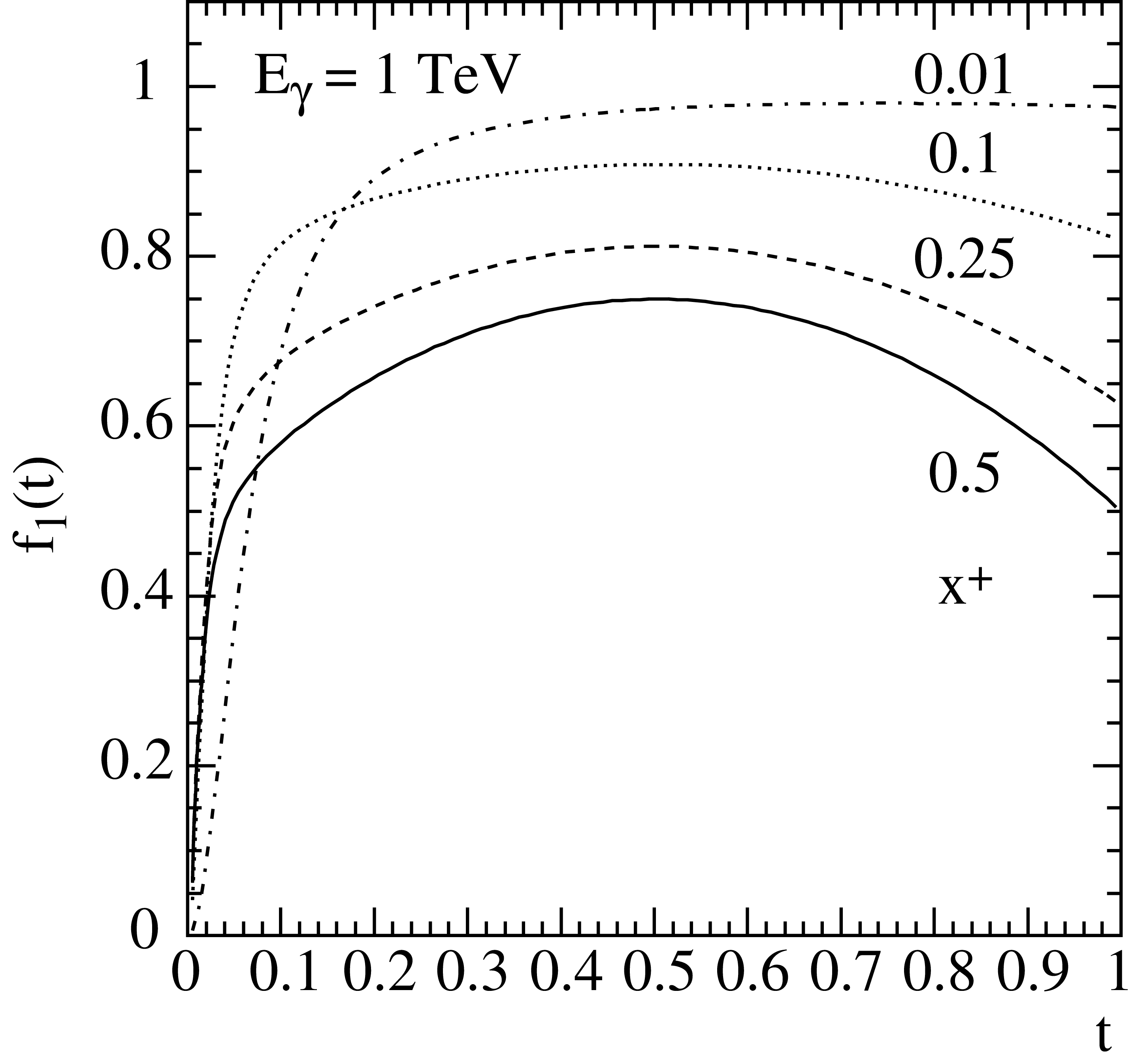
Fig. 8 The function \(f_1(t)\) at \(E_{\gamma} = 1\,{\rm TeV}\) in beryllium for different values of \(x_+\).
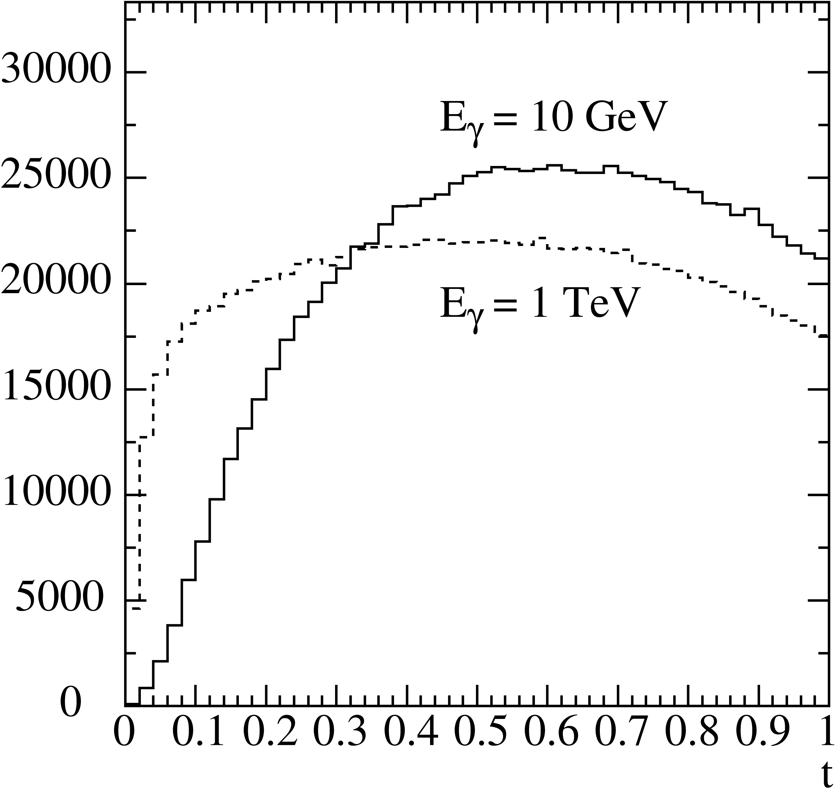
Fig. 9 Histograms of generated \(t\) distributions for \(E_{\gamma} = 10\,{\rm GeV}\) (solid line) and \(E_{\gamma} = 100\,{\rm GeV}\) (dashed line) with \(10^6\) events each.
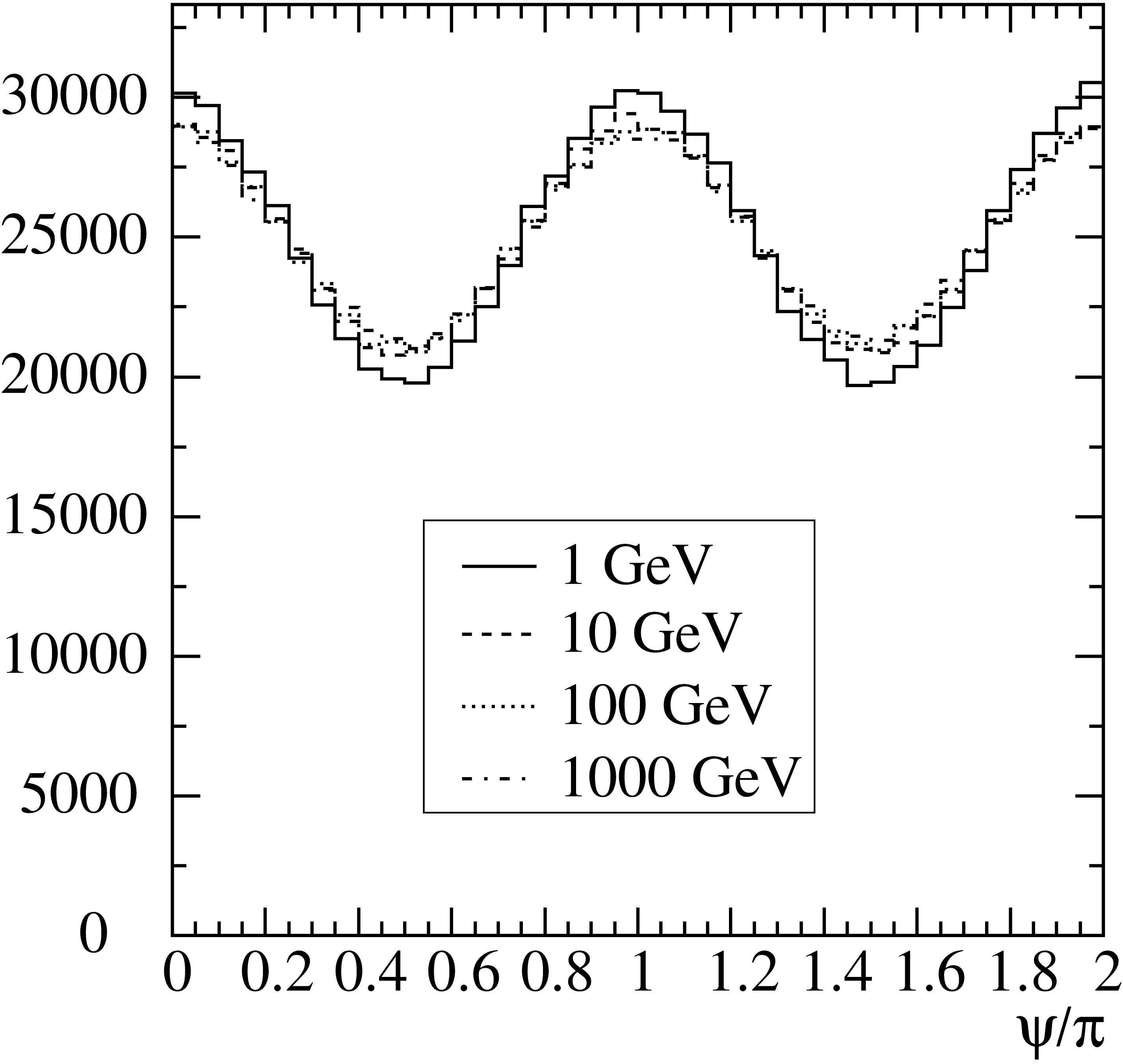
Fig. 10 Histograms of generated \(\psi\) distributions for beryllium at four different photon energies.
The Monte Carlo generation is done using the rejection technique. About 70% of the generated numbers are kept in this step. Generated \(t\)-distributions are shown in Fig. 9.
Generate \(\psi\) by the rejection technique using \(t\) generated in the previous step for the frequency distribution
\[f_2(\psi) =\Big[1-2\,x_+x_{-}+4\,x_+x_{-}t\,(1-t)\,(1+\cos(2\psi))\Big]\;, \qquad 0\le\psi\le2\pi\,.\]The maximum of \(f_2(\psi)\) is
\[\max [f_2(\psi)]=1-2\,x_+x_-\left[1-4\,t\,(1-t)\right]\,.\,\]Generated distributions in \(\psi\) are shown in Fig. 10.
Generate \(\rho\). The distribution in \(\rho\) has the form
\[f_3(\rho)\,d\rho=\frac{\rho^3\,d\rho}{\rho^4+C_2}\,,\quad 0\le\rho\le \rho_{\rm max}\,,\,\]where
\[\rho_{\rm max}^2=\frac{1.9}{A^{0.27}}\,\left(\frac{1}{t}-1\right), \,\]and
\[C_2=\frac4{\sqrt{x_+x_-}}\left[\left(\frac{m_\mu}{2E_\gamma x_+x_-\,t} \right)^2+\left(\frac{m_e}{183 \, Z^{-1/3} \, m_\mu}\right)^2 \right]^2\,.\]The \(\rho\) distribution is obtained by a direct transformation applied to uniform random numbers \(R_i\) according to
\[\rho=\left[C_2(\exp(\beta\,R_i)-1)\right]^{1/4}\,,\]where
\[\beta=\log\left(\frac{C_2+\rho_{\rm max}^4}{C_2}\right)\,.\]Generated distributions of \(\rho\) are shown in Fig. 11
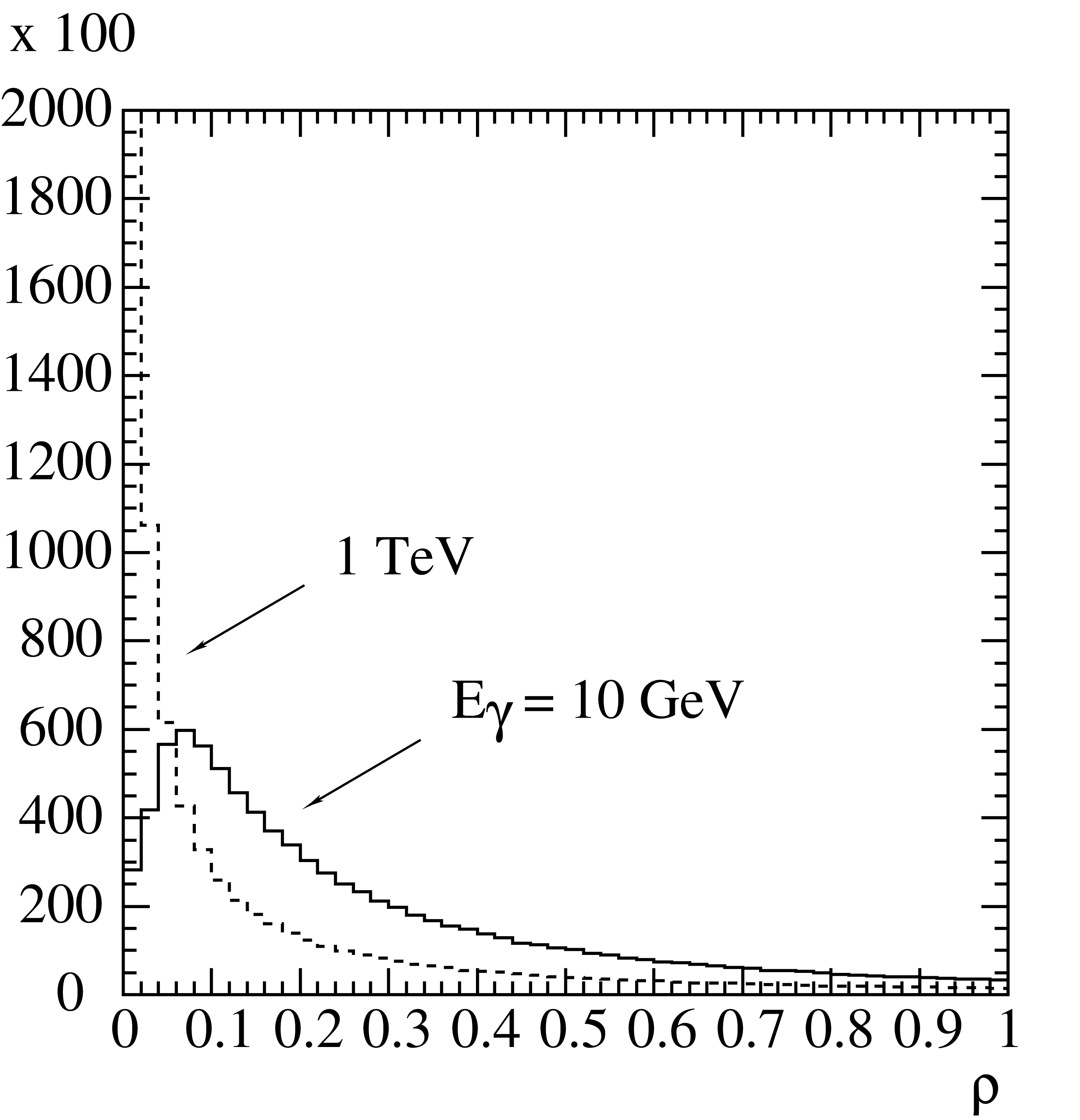
Fig. 11 Histograms of generated \(\rho\) distributions for beryllium at two different photon energies. The total number of entries at each energy is \(10^6\).
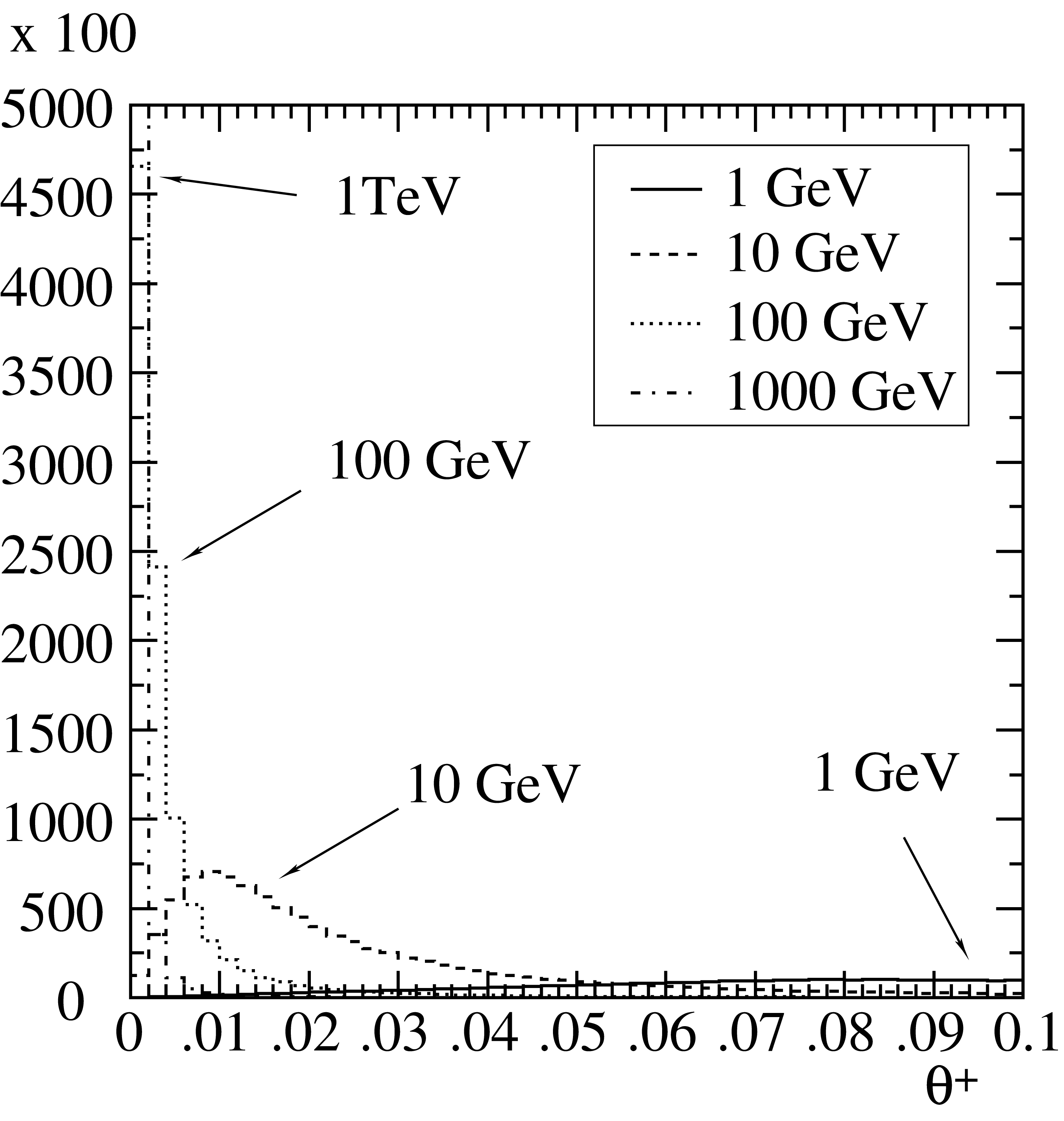
Fig. 12 Histograms of generated \(\theta_+\) distributions at different photon energies.
Calculate \(\theta_+,\theta_-\) and \(\varphi\) from \(t, \rho,\psi\) with
(28)\[\gamma_{\pm} = \frac{E_{\mu}^\pm}{m_{\mu}} \qquad {\rm and} \qquad u=\sqrt{\frac1t-1}\,.\]according to
\[\theta_+= \frac{1}{\gamma_+}\,\left(u +\frac{\rho}{2}\,\cos\psi\right)\,,\quad \theta_-= \frac{1}{\gamma_-}\,\left(u -\frac{\rho}{2}\,\cos\psi\right)\, \quad {\rm and} \quad \varphi=\frac{\rho}{u} \, \sin\psi\, . \,\]The muon vectors can now be constructed from Eq.(24), where \(\varphi_0\) is chosen randomly between 0 and \(2\pi\). Fig. 12 shows distributions of \(\theta_+\) at different photon energies (in beryllium). The spectra peak around \(1/\gamma\) as expected.
The most probable values are \(\theta_+\sim m_\mu/E_\mu^+ = 1 / \gamma_+\). In the small angle approximation used here, the values of \(\theta_+\) and \(\theta_-\) can in principle be any positive value from 0 to \(\infty\). In the simulation, this may lead (with a very small probability, of the order of \(m_\mu/E_\gamma\)) to unphysical events in which \(\theta_+\) or \(\theta_-\) is greater than \(\pi\). To avoid this, a limiting angle \(\theta_{\rm cut}=\pi\) is introduced, and the angular sampling repeated, whenever \(\max(\theta_+,\,\theta_-)>\theta_{\rm cut}\).
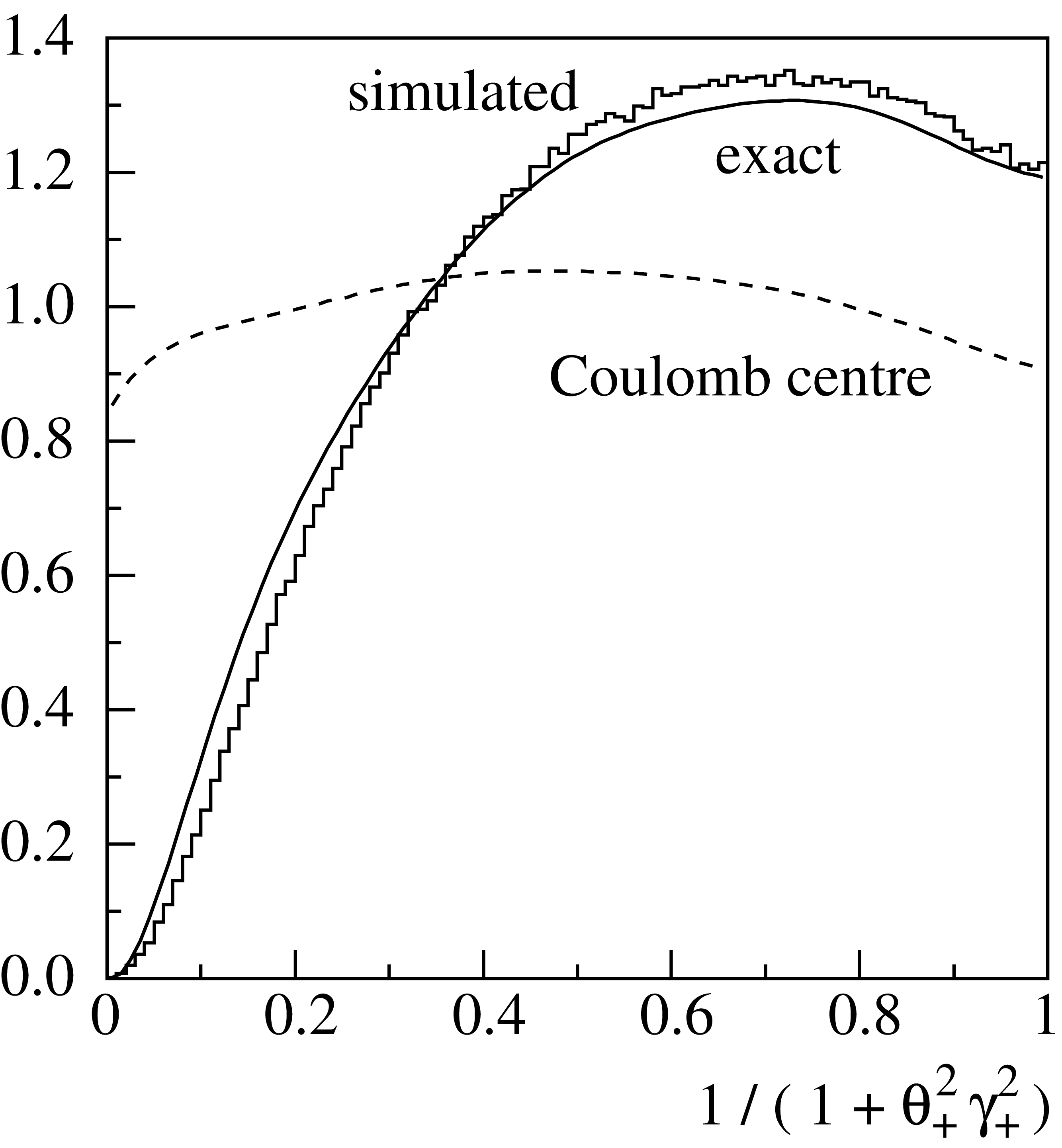
Fig. 13 Angular distribution of positive (or negative) muons. The solid curve represents the results of the exact calculations. The histogram is the simulated distribution. The angular distribution for pairs created in the field of the Coulomb centre (point-like target) is shown by the dashed curve for comparison.
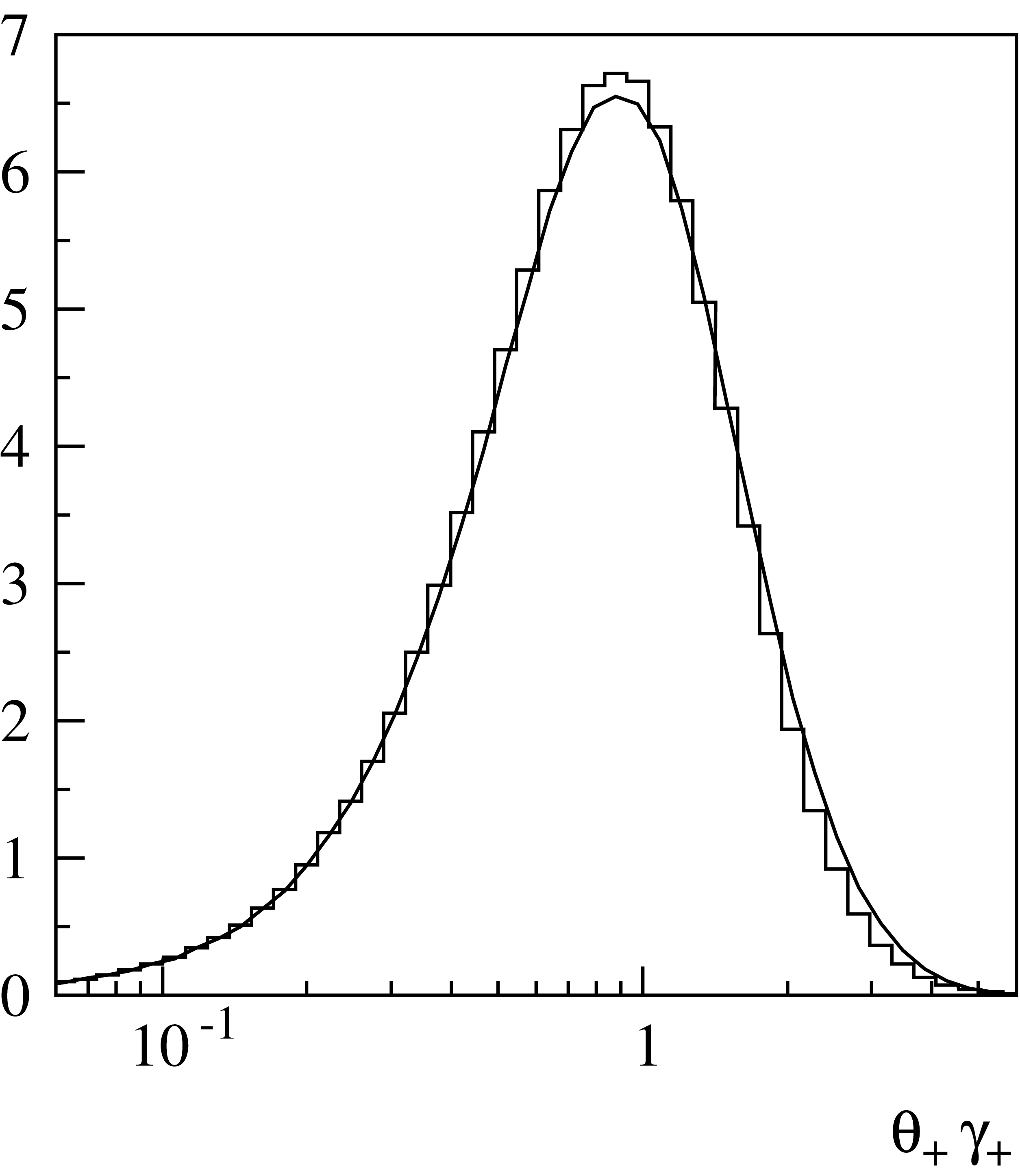
Fig. 14 Angular distribution in logarithmic scale. The curve corresponds to the exact calculations and the histogram is the simulated distribution.
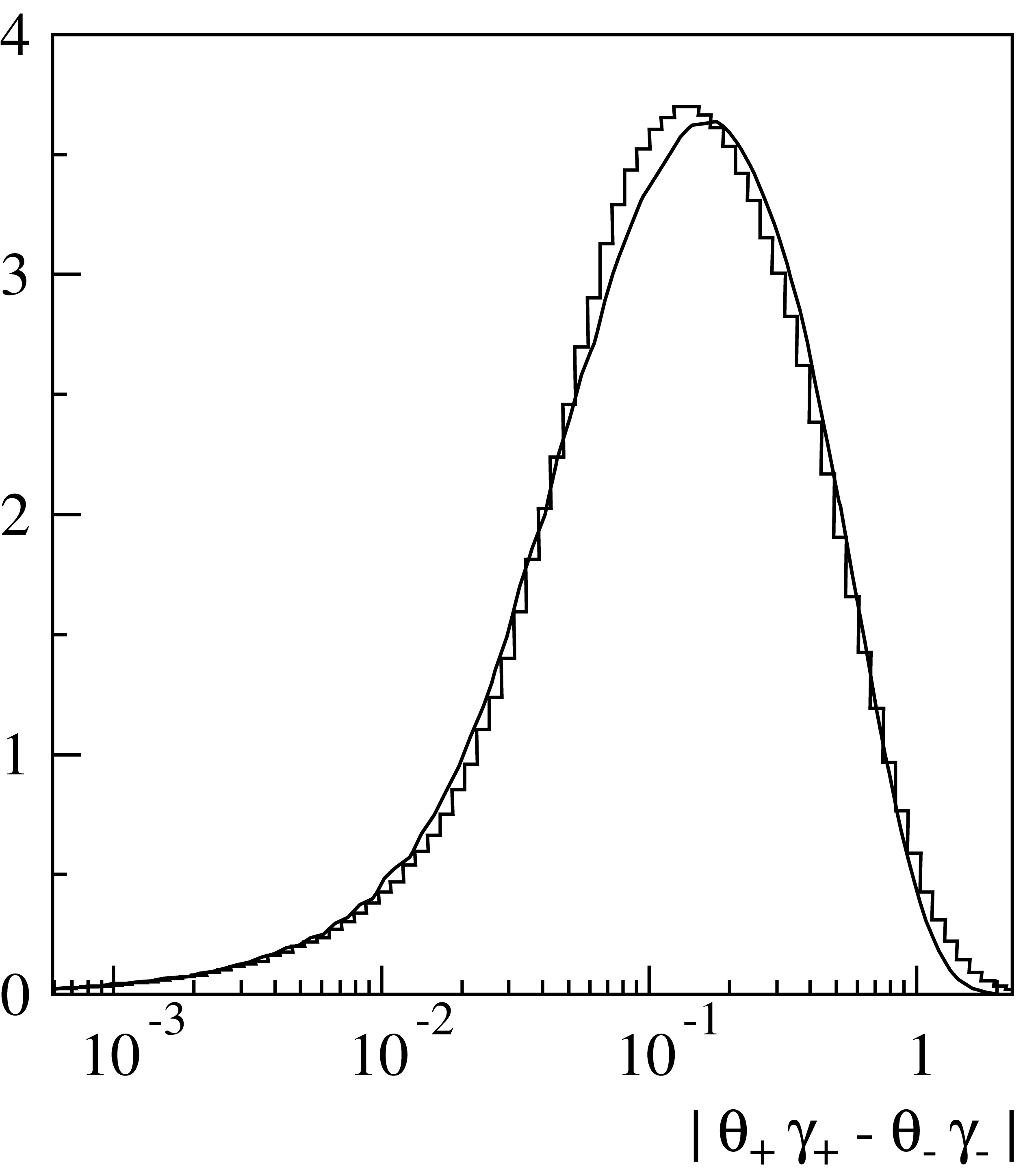
Fig. 15 Distribution of the difference of transverse momenta of positive and negative muons (with logarithmic x-scale).
Fig. 13, Fig. 14 and Fig. 15 show distributions of the simulated angular characteristics of muon pairs in comparison with results of exact calculations. The latter were obtained by means of numerical integration of the squared matrix elements with respective nuclear and atomic form factors. All these calculations were made for iron, with \(E_\gamma=10\,{\rm GeV}\) and \(x_+=0.3\). As seen from Fig. 13, wide angle pairs (at low values of the argument in the figure) are suppressed in comparison with the Coulomb center approximation. This is due to the influence of the finite nuclear size which is comparable to the inverse mass of the muon. Typical angles of particle emission are of the order of \(1/\gamma_\pm=m_\mu/E_\mu^\pm\) (Fig. 14). Fig. 15 illustrates the influence of the momentum transferred to the target on the angular characteristics of the produced pair. In the frame of the often used model which neglects target recoil, the pair particles would be symmetric in transverse momenta, and coplanar with the initial photon.
Five-dimensional (5D) Bethe-Heitler gamma Conversion to \(\mu ^+\mu ^-\)
Since release 10.6, the G4BetheHeitler5DModel physics model for
\(\gamma\)-ray conversions to e+e- pairs (section Five-dimensional (5D) Bethe-Heitler gamma Conversion to e+e-) has been
extended to the conversions to \(\mu^+\mu^-\) pairs, sampling the 5D
Bethe-Heitler differential cross section as described in the preceding section.
For decays to muon pairs, G4BetheHeitler5DModel is a low-energy complement to the
former G4GammaConversionToMuons model that is using high-energy approximations,
that has been verified above 10 GeV and that is described above (em.gmumu).
G4BetheHeitler5DModel is expected to be valid down to threshold and the
algorithm has been verified down to a couple of hundred keV above
threshold [Ber19]. Conversions of linearly
polarised or non-polarised incident photons can be generated. The energy
threshold is
where M is the target mass.
For triplet conversion (\(\gamma ~ e^{-} ~ \to ~ \mu^{+}\mu^{-} ~ e^{-}\)), \(E_{\text{threshold}}\) is close to 44 GeV.
For nuclear conversion (\(\gamma ~ Z ~ \to ~ \mu^{+}\mu^{-} ~ Z\)), \(E_{\text{threshold}}\) ranges from 223 MeV for hydrogen targets down to almost \(2 m_{\mu} c^{2} \approx 211\) MeV for heavy nuclei.
Fig. 16 presents distributions of kinematic variables of interest for several incident-photon energies for \(\gamma\)-ray nuclear conversion on Argon:
\(\theta_{\mu^{+}\mu^{-}} \times E\), the pair opening angle multiplied by the incident-photon energy; the vertical line shows the most probable value of the distribution, \(3.2 m_{\mu} c^2\), obtained by Olsen in the high-energy approximation [Ols63];
\(\log_{10}{(q)}\), where q is the (nucleus) recoil momentum;
\(\phi_{\text{recoil}}\), azimutal angle of the (nucleus) recoil momentum (for a fully linearly polarized \(\gamma\)-ray beam);
\(E_{\mu^{+}} / E\), the fraction of the incident-photon energy that is carried away by the positive muon
Note that G4BetheHeitler5DModel does not take the finite size of the nucleus into account.
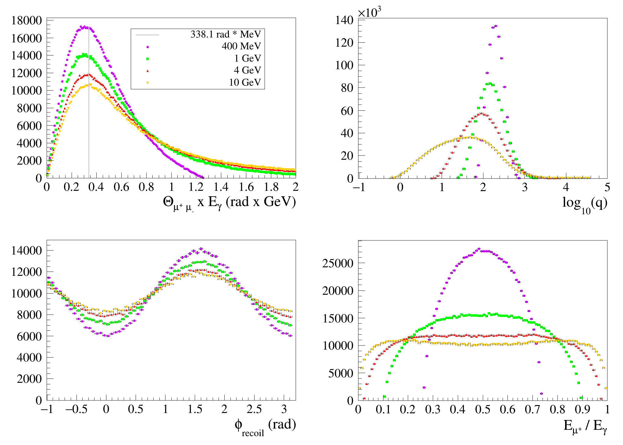
Fig. 16 G4BetheHeitler5DModel: \(\gamma\)-ray conversions to \(\mu^+\mu^-\) pairs on Argon atoms (see text), for various incident-photon energies (bullets 400 MeV, squares 1 GeV, upper triangle 4 GeV, down triangle 10 GeV).
Bibliography
- Ber19
Denis Bernard. A 5d, polarised, bethe-heitler event generator for $\gamma$ to $\mu $$\mathplus $$\mu $- conversion. 2019. arXiv:1910.12501.
- BKK02
H Burkhardt, S R Kelner, and R P Kokoulin. Monte carlo generator for muon pair production. Technical Report CERN-SL-2002-016-AP. CLIC-Note-511, CERN, Geneva, May 2002. URL: https://cds.cern.ch/record/558831.
- KKP95
SR Kelner, RP Kokoulin, and AA Petrukhin. About cross section for high-energy muon bremsstrahlung. Technical Report, MEphI, 1995. Preprint MEPhI 024-95, Moscow, 1995, CERN SCAN-9510048.
- Ols63
Haakon Olsen. Opening Angles of Electron-Positron Pairs. Phys. Rev., 131:406–415, 1963.