Introduction

The Fritiof model, or FTF for short, is used in Geant4 for simulation of the following interactions: hadron-nucleus at P_lab > 3–4 GeV/c, nucleus-nucleus at P_lab > 2–3 GeV/c/nucleon, antibaryon-nucleus at all energies, and antinucleus-nucleus. Because the model does not include multi-jet production in hadron-nucleon interactions, the upper limit of its validity range is estimated to be 1000 GeV/c per hadron or nucleon.

The model assumes that one or two unstable objects (quark-gluon strings) are produced in elementary interactions. If only one object is created, the process is called diffraction dissociation. It is assumed also that the objects can interact with other nucleons in hadron-nucleus and nucleus-nucleus collisions, and can produce other objects. The number of produced objects in these non-diffractive interactions is proportional to the number of participating nucleons. Thus, multiplicities in the hadron-nucleus and nucleus-nucleus interactions are larger than those in elementary ones.

The modeling of hadron-nucleon interactions in the FTF model includes simulations of elastic scattering, binary reactions like \(NN\rightarrow N\Delta\), \(\pi N\rightarrow \pi \Delta\), single diffractive and non-diffractive events, and annihilation in antibaryon-nucleon interactions. It is assumed that the unstable objects created in hadron-nucleus and nucleus-nucleus collisions can have analogous reactions.

Parameterizations of the CHIPS Geant4 model are used for calculations of elastic and inelastic hadron-nucleon cross sections. Data-driven parameterizations of the binary reaction cross sections and the diffraction dissociation cross sections in the elementary interactions are implemented in the FTF model. It is assumed in the model that the unstable object cross sections are equal to the cross sections of stable objects having the same quark content.

The LUND string fragmentation model is used for the simulation of unstable object decays. The formation time of hadrons is considered also. Parameters of the fragmentation model were tuned to experimental data. A restriction of the available phase space is taken into account in low mass string fragmentation.

A simplified Glauber model is used for sampling the multiplicity of intra-nuclear collisions. Gribov inelastic screening is not considered. For medium and heavy nuclei a Saxon-Woods parameterization of the one-particle nuclear density is used, while for light nuclei a harmonic oscillator shape is used. Center-of-mass correlations and short range nucleon-nucleon correlations are taken into account.

The reggeon theory inspired model (RTIM) of nuclear destruction is applied for a description of secondary particle intra-nuclear cascading. A new algorithm to simulate “Fermi motion” in nuclear reactions is used.

Excitation energies of residual nuclei are estimated in the wounded nucleon approximation. This allows for a direct coupling of the FTF model to the Precompound model of Geant4 and hence with the GEM nuclear fragmentation model. The determination of the particle formation time allows one to couple the FTF model with the Binary cascade model of Geant4 (The Binary Cascade Model).

Main assumptions of the FTF model

The Fritiof model [eal87][BNilssonAEStenlund87] assumes that all hadron-hadron interactions are binary reactions, \(h_1+h_2\rightarrow h_1'+h_2'\), where \(h_1'\) and \(h_2'\) are excited states of the hadrons with discrete or continuous mass spectra (see Fig. 75). If one of the final hadrons is in its ground state (\(h_1+h_2\rightarrow h_1+h_2'\)) the reaction is called “single diffraction dissociation”, and if neither hadron is in its ground state it is called a “non-diffractive” interaction. (Notice that, in spite of its name, this definition of “non-diffractive” interaction includes the double diffraction dissociation as well.)

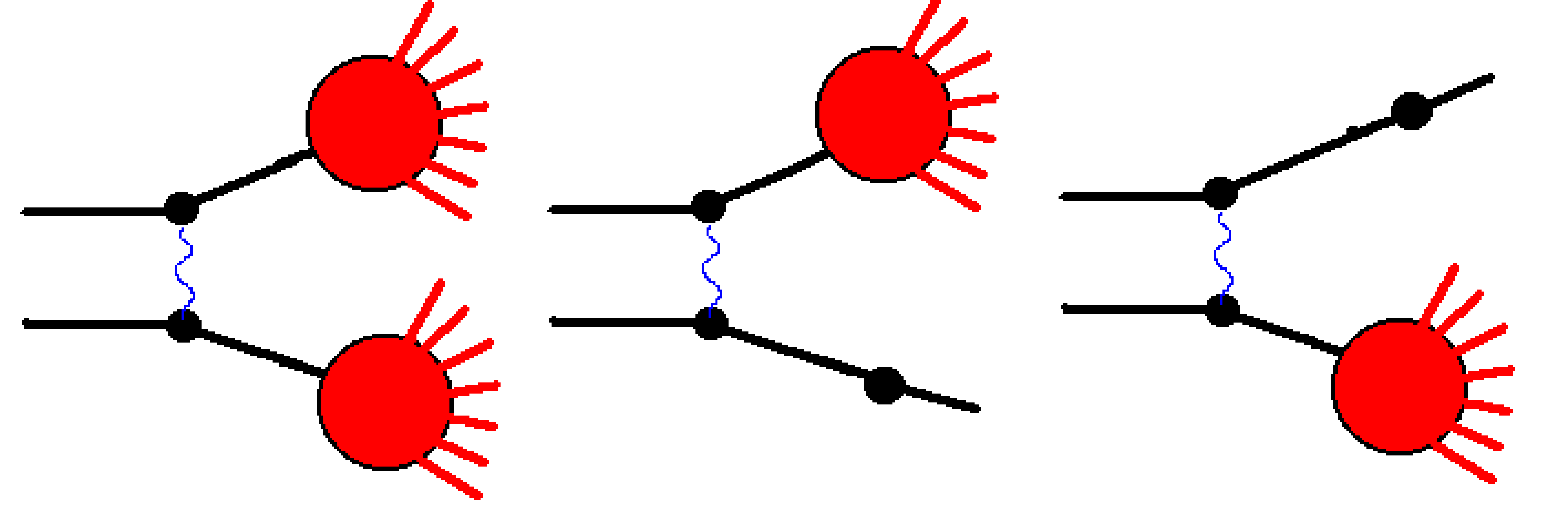
Fig. 75 Non-diffractive and diffractive interactions considered in the Fritiof model.

The excited hadrons are considered as QCD-strings, and the corresponding LUND-string fragmentation model is applied in order to simulate their decays.

The key ingredient of the Fritiof model is the sampling of the string masses. In general, the set of final state of interactions can be represented by Fig. 76, where samples of possible string masses are shown. There is a point corresponding to elastic scattering, a group of points which represents final states of binary hadron-hadron interactions, lines corresponding to the diffractive interactions, and various intermediate regions. The region populated with the red points is responsible for the non-diffractive interactions. In the model, the mass sampling threshold is set equal to the ground state hadron masses, but in principle the threshold can be lower than these masses. The string masses are sampled in the triangular region restricted by the diagonal line corresponding to the kinematical limit \(M_1+M_2=E_{cms}\) where \(M_1\) and \(M_2\) are the masses of the \(h_1'\) and \(h_2'\) hadrons, and also of the threshold lines. If a point is below the string mass threshold, it is shifted to the nearest diffraction line.

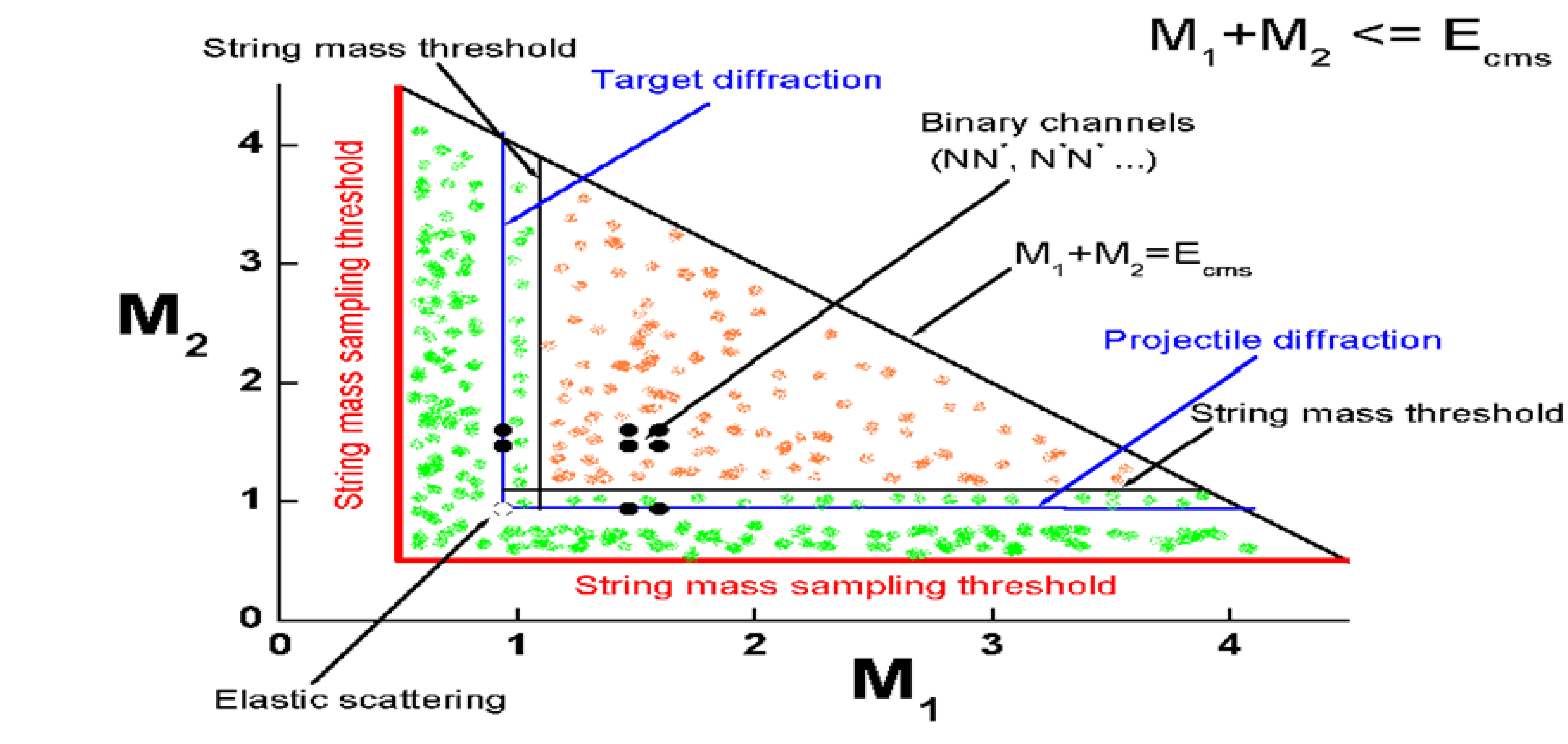
Fig. 76 Diagram of the final states of hadron-hadron interactions.

Unlike the original Fritiof model, the final state diagram of the current model is complicated, which leads to a mass sampling algorithm that is not simple. This will be considered below. The original model had no points corresponding to elastic scattering or to the binary final states. As it was known at the time, the mass of an object produced by diffraction dissociation, \(M_x\), for example from the reaction \(p+p\rightarrow p+X\), is distributed as \(dM_x/M_x\propto dM^2_x/M^2_x\), so it was natural to assume that the object mass distributions in all inelastic interactions obeyed the same law. This can be re-written using the light-cone momentum variables, \(P^+\) or \(P^-\),

\[P^+=E+p_z ,\ \ \ P^-=E-p_z\]

where \(E\) is an energy of a particle, and \(p_z\) is its longitudinal momentum along the collision axis. At large energy and positive \(p_z\), \(P^-\simeq (M^2+P_T^2)/2p_z\). At negative \(p_z\), \(P^+\simeq (M^2+P_T^2)/2|p_z|\). Usually, the transferred transverse momentum, \(P_T\), is small and can be neglected. Thus, it was assumed that \(P^-\) and \(P^+\) of a projectile, or target associated hadron, respectively, are distributed as

\[dP^-/P^- ,\ \ \ dP^+/P^+\]

A gaussian distribution was used to sample \(P_T\).

In the case of hadron-nucleus or nucleus-nucleus interactions it was assumed that the created objects can interact further with other nuclear nucleons and create new objects. Assuming equal masses of the objects, the multiplicity of particles produced in these interactions will be proportional to the number of participating nuclear nucleons, or to the multiplicity of intra-nuclear collisions. Due to this, the multiplicity of particles produced in hadron-nucleus or nucleus-nucleus interactions is larger than that in hadron-hadron ones. The probabilities of multiple intra-nuclear collisions were sampled with the help of a simplified Glauber model. Cascading of secondary particles was not considered.

Because the Fermi motion of nuclear nucleons was simulated in a simple manner, the original Fritiof model could not work at \(P_{lab} <\) 10–20 GeV/c.

It was assumed in the model that the created objects are quark-gluon strings with constituent quarks at their ends originating from the primary colliding hadrons. Thus, the LUND-string fragmentation model was applied for a simulation of the object decays. It was assumed also that the strings with sufficiently large masses have “kinks” – additional radiated gluons. This was very important for a correct reproduction of particle multiplicities in the interactions.

All of the above assumptions were reconsidered in the implementation of the Geant4 Fritiof model, and new features were added. These will be presented below.

General properties of hadron–nucleon interactions

Before going into details of the FTF model implementation it would be better to consider briefly the general properties of hadron-nucleon interactions in order to understand what needs to be simulated. These properties include total and elastic cross sections, and cross sections of various other reactions. There is so much data on inclusive spectra that not all of it can be addressed in this work. It is hoped that the remaining data will be the subject of a future paper. Inclusive data present kinematical properties of produced particles. Their description requires additional methods and parameters, which will be considered later.

\(\pi^- p\) interactions

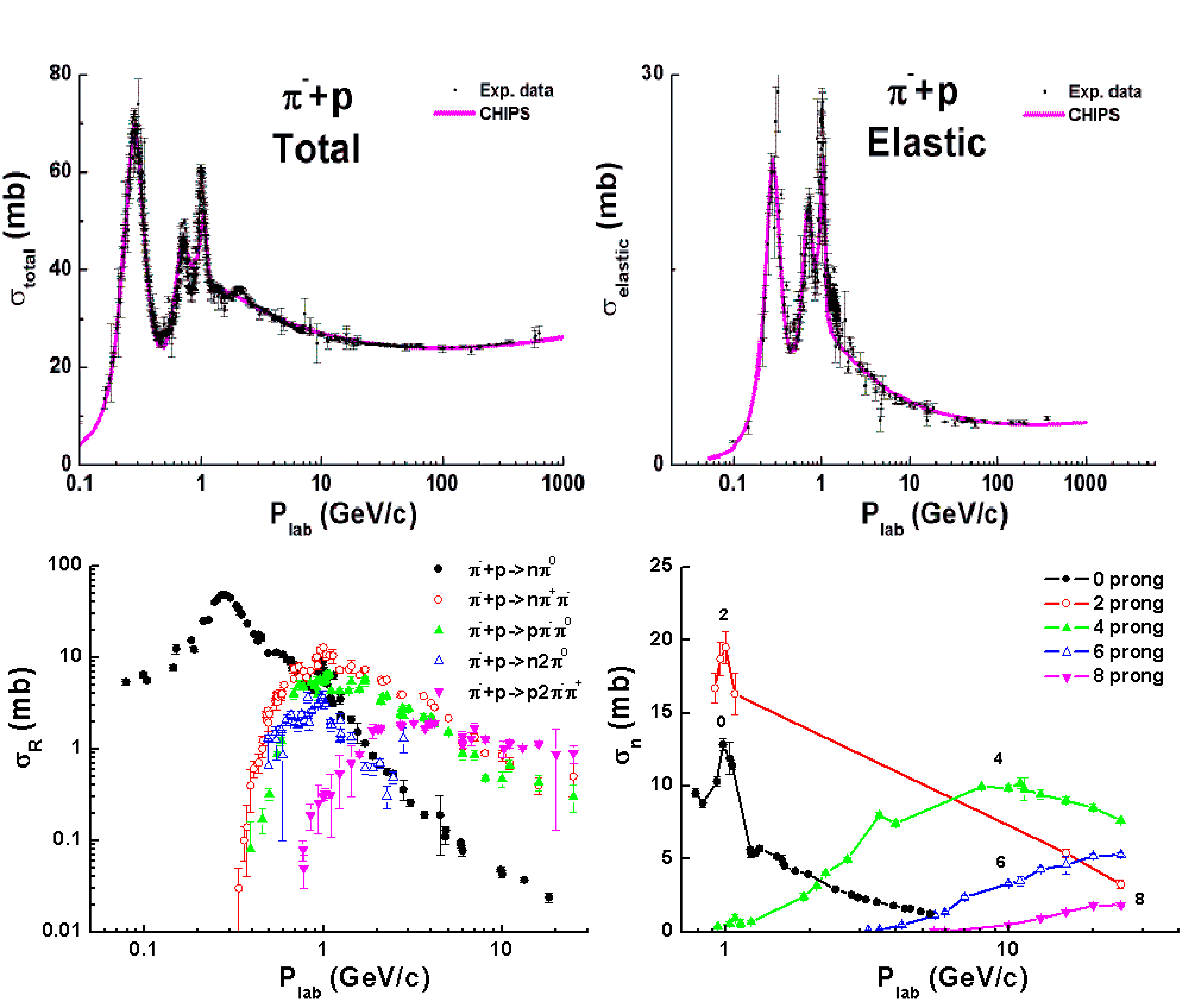
Fig. 77 General properties of \(\pi^-p\)-interactions. Points are experimental data: data on total and elastic cross sections from PDG data-base [PDG12], other data from [eal72].

Total, elastic and reaction cross sections of \(\pi^-p\)-interactions are presented in Fig. 77. As seen, there are peaks in the total cross section connected with \(\Delta\)-isobar production (\(\Delta(1232)\), \(\Delta(1600)\), \(\Delta(1700)\) and so on) in the \(s\)-channel, \(\pi^-+p\rightarrow \Delta^0\). The main channel of a \(\Delta^0\)-isobar decay is \(\Delta^0 \rightarrow \pi^-+p\). These resonances are reflected in the elastic cross section. The other important decay channel is \(\Delta^0 \rightarrow \pi^0+n\), which is the main inelastic reaction channel at \(P_{lab}<\) 700 MeV/c. At higher energy two-meson production channels start to dominate, and at \(P_{lab}>\) 3 GeV/c there is practically no structure in the cross sections. Cross sections of final states with defined charged particle multiplicity, so-called prong cross sections according to the old terminology, are presented in the last figure. As seen, real multi-particle production processes (\(n\geq 4\)) dominate at \(P_{lab}>\) 5–7 GeV/c.

In the constituent quark model of hadrons, the creation of \(s\)-channel \(\Delta\)-isobars is explained by quark–antiquark annihilation (see Fig. 78a). The production of two mesons may result from quark exchange (see Fig. 78b, Fig. 78c). A quark–diquark (\(q\)–\(qq\)) system created in the process can be in a resonance state (Fig. 78b), or in a state with a continuous mass spectrum (Fig. 78c). In the latter case, multi-meson production is possible. Amplitudes of these two channels are connected by crossing symmetry to annihilation in the \(t\)-channel, and with non-vacuum exchanges in the elastic scattering according to the reggeon phenomenology. According to that phenomenology, pomeron exchange must dominate in elastic scattering at high energies. In a simple approach, this corresponds to two-gluon exchange between colliding hadrons. It reflects also one or many non-perturbative gluon exchanges in the inelastic reaction. Due to these exchanges, a state with subdivided colors is created (see Fig. 78d). The state can decay into two colorless objects. The quark content of the objects coincides with the quark content of the primary hadrons, according to the FTF model, or it is a mixture of the primary hadron’s quarks, according to the Quark-Gluon-String model (QGSM).

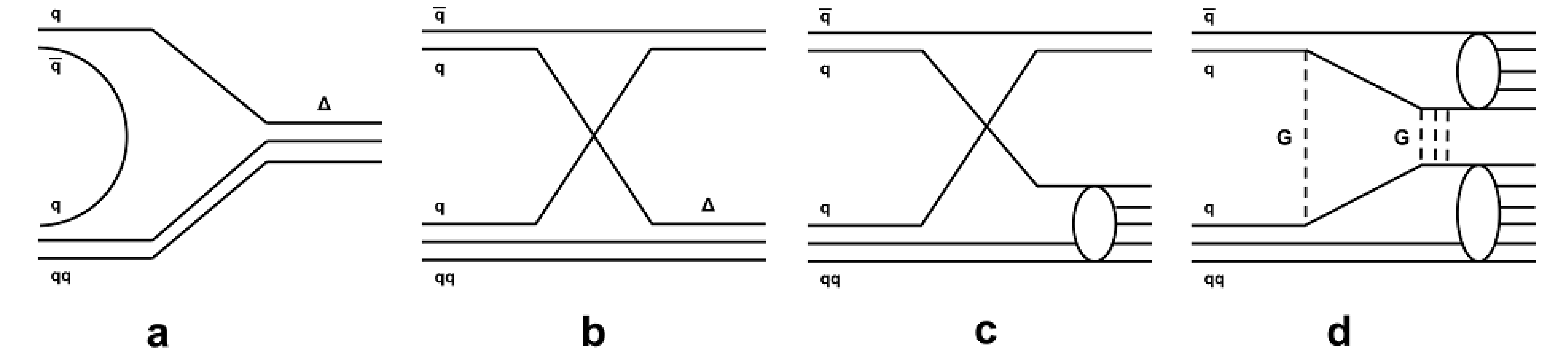
Fig. 78 Quark flow diagrams of \(\pi N\)-interactions.

The original Fritiof model contains only the pomeron exchange process shown in Fig. 78d. It would be useful to extend the model by adding the exchange processes shown in Fig. 78b and Fig. 78c, and the annihilation process of Fig. 78a. This could probably be done by introducing a restricted set of mesonic and baryonic resonances and a corresponding set of parameters. This procedure was employed in The Binary Cascade Model of Geant4 (BIC) [FIW04] and in the Ultra-Relativistic-Quantum-Molecular-Dynamic model (UrQMD) [eal98][eal99] (see Quantum Molecular Dynamics for Heavy Ions). However, it is complicated to use this solution for a simulation of hadron-nucleus and nucleus-nucleus interactions. The problem is that one has to consider resonance propagation in the nuclear medium and take into account their possible decays which enormously increases computing time. Thus, in the current version of the FTF model only quark exchange processes have been added to account for meson and baryon interactions with nucleons, without considering resonance propagation and decay. This is a reasonable hypothesis at sufficiently high energies.

\(\pi^+ p\) interactions

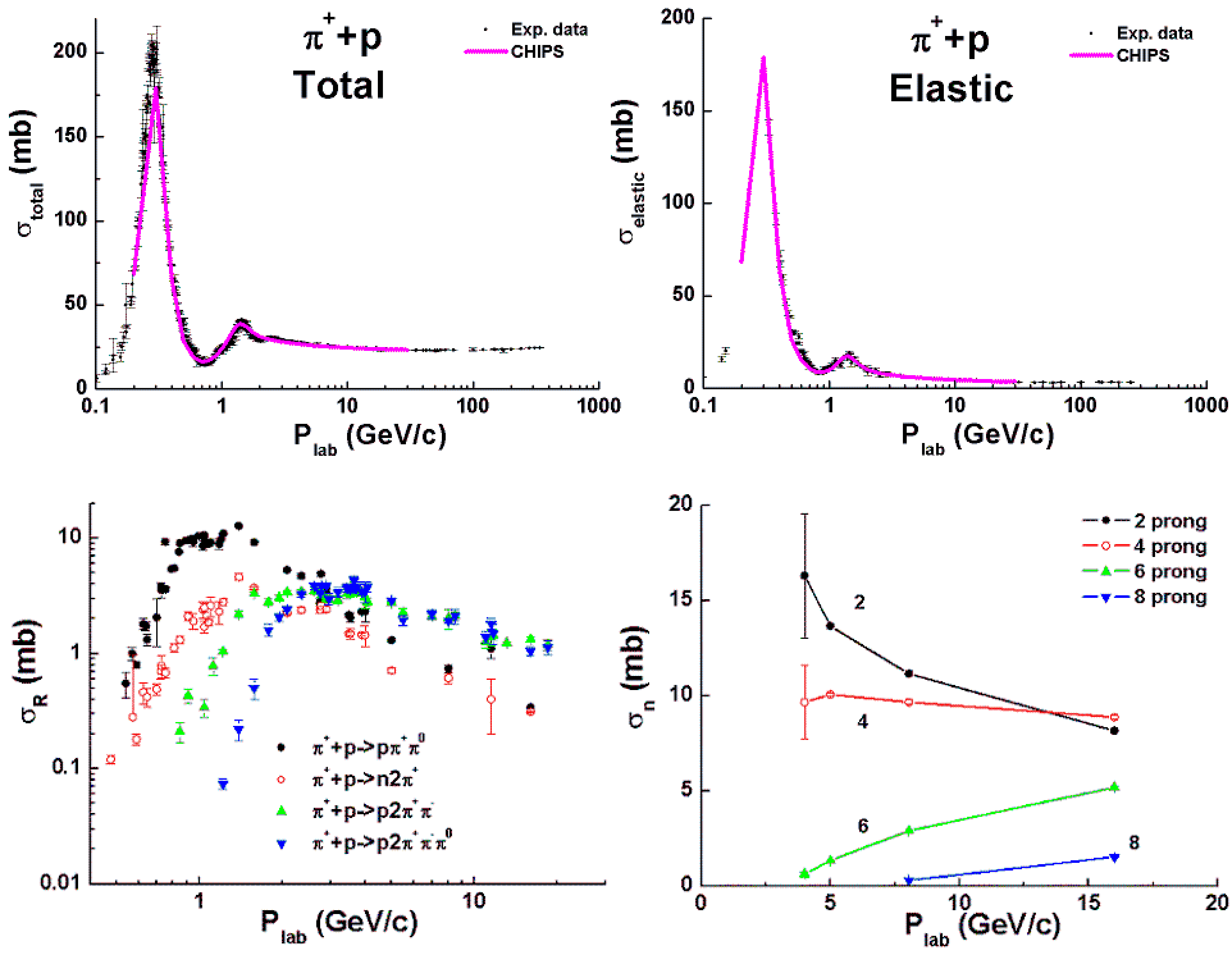
Fig. 79 General properties of \(\pi^+p\)-interactions. Points are experimental data: data on total and elastic cross sections from PDG data-base [PDG12], other data from [eal72].

Total, elastic and reaction cross sections of \(\pi^+p\)-interactions are presented in Fig. 79. As seen, there are fewer peaks in the total cross section than in \(\pi^-p\)-collisions. The creation of \(\Delta^{++}\)-isobars in the \(s\)-channel (\(\pi^++p\rightarrow \Delta^{++}\)) is mainly seen in the elastic cross section because the main channel of \(\Delta^{++}\)-isobar decay is \(\Delta^{++} \rightarrow \pi^++p\). This process is due to quark–antiquark annihilation. At \(P_{lab}>\) 400 MeV/c two-meson production channels appear. They can be connected with quark exchange and with the formation of \(\Delta^{++}\) and \(\Delta^{+}\) isobars at the proton site. The corresponding cross sections of the reactions – \(\pi^++p\rightarrow \pi^0+\Delta^{++}\rightarrow \pi^0+\pi^{+}+p\), \(\pi^++p\rightarrow \pi^++\Delta^{+}\rightarrow \pi^++\pi^{0}+p\), \(\pi^++p\rightarrow \pi^++\Delta^{+}\rightarrow \pi^++\pi^{+}+n\) have structures at \(P_{lab} \simeq \) 1.5 and 2.8 GeV/c. At higher energies there is no structure. The cross sections of other reactions are rather smooth.

\(p p\) interactions

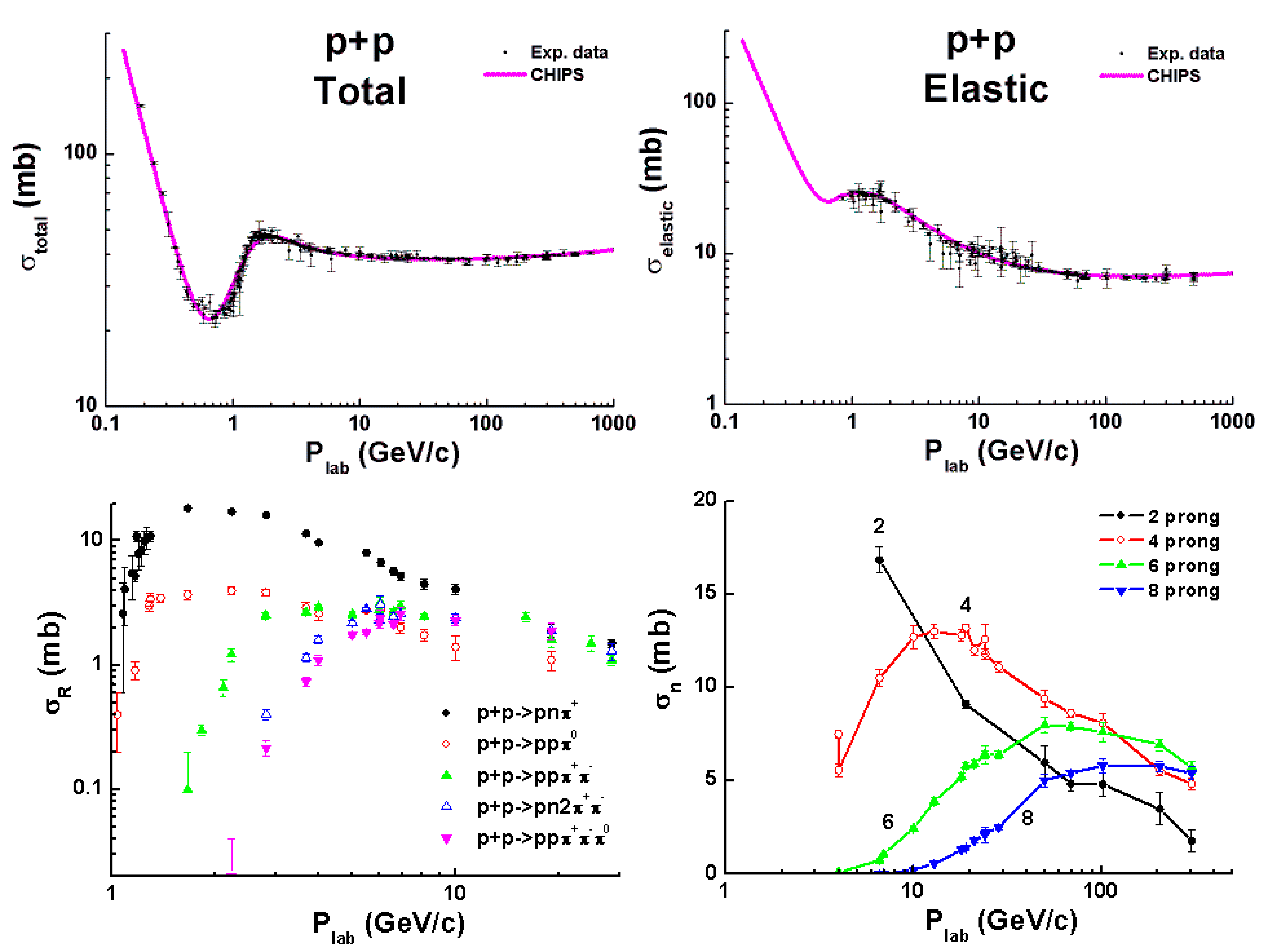
Fig. 80 General properties of \(pp\)-interactions. Points are experimental data: data on total and elastic cross sections from PDG data-base [PDG12], other data from [eal73a][eal84].

Total, elastic and reaction cross sections of \(pp\)-interactions are presented in Fig. 80. The total cross section is seen to decrease with energy below the meson production threshold (\(P_{lab}\leq\) 800 MeV/c). Above the threshold the cross section starts to increase and becomes nearly constant. The main reaction channel below 6–8 GeV/c is \(p+p\rightarrow p+n+\pi^+\). Because there cannot be quark–antiquark annihilation in the interaction, the reaction must be connected to quark exchange. Intermediate states can be \(p+p\rightarrow p+\Delta^+\) and \(p+p\rightarrow n+\Delta^{++}\). In the first case, quarks of the same flavor in the projectile and the target are exchanged. In the second case quarks with different flavors take part in the exchange. Because the cross section of the \(p+p\rightarrow p+n+\pi^+\) reaction is larger than the that of \(p+p\rightarrow p+p+\pi^0\), one has to assume that the exchange of quarks with the same flavors is suppressed.

All the reactions shown can also be caused by diffraction dissociation. Although there can be a contribution of the \(p+p\rightarrow \Delta^0+\Delta^{++}\) reaction into the cross section of the channel \(p+p\rightarrow (p+\pi^-)+(p+\pi^+)\) at \(P_{lab} \sim\) 2–3 GeV/c, one can assume that diffraction plays an essential role in these interactions, because there are no defined structures in the cross sections.

Summing up the consideration of the interactions, one can conclude that the probability of quark exchanges can depend on quark flavors, and that \(pp\)-collisions could be a source of information about diffraction.

\(K^+ p\) – and \(K^- p\) interactions

For completeness, the properties of \(K^+p\)- and \(K^-p\)-interactions are presented. Total and elastic cross sections are shown in Fig. 81. As the \(s\)-antiquark in the \(K^+\)-mesons cannot annihilate in the \(K^+p\)-interactions, the structure of the corresponding cross sections is rather simple, and is very like the structure of \(pp\) cross sections. The \(u\)-antiquark in the \(K^-\)-mesons can annihilate, and the structure of the cross sections is more complicated. Due to these features, inelastic reactions are very different even though all of them can be connected with various quark flow diagrams like that shown in Fig. 78

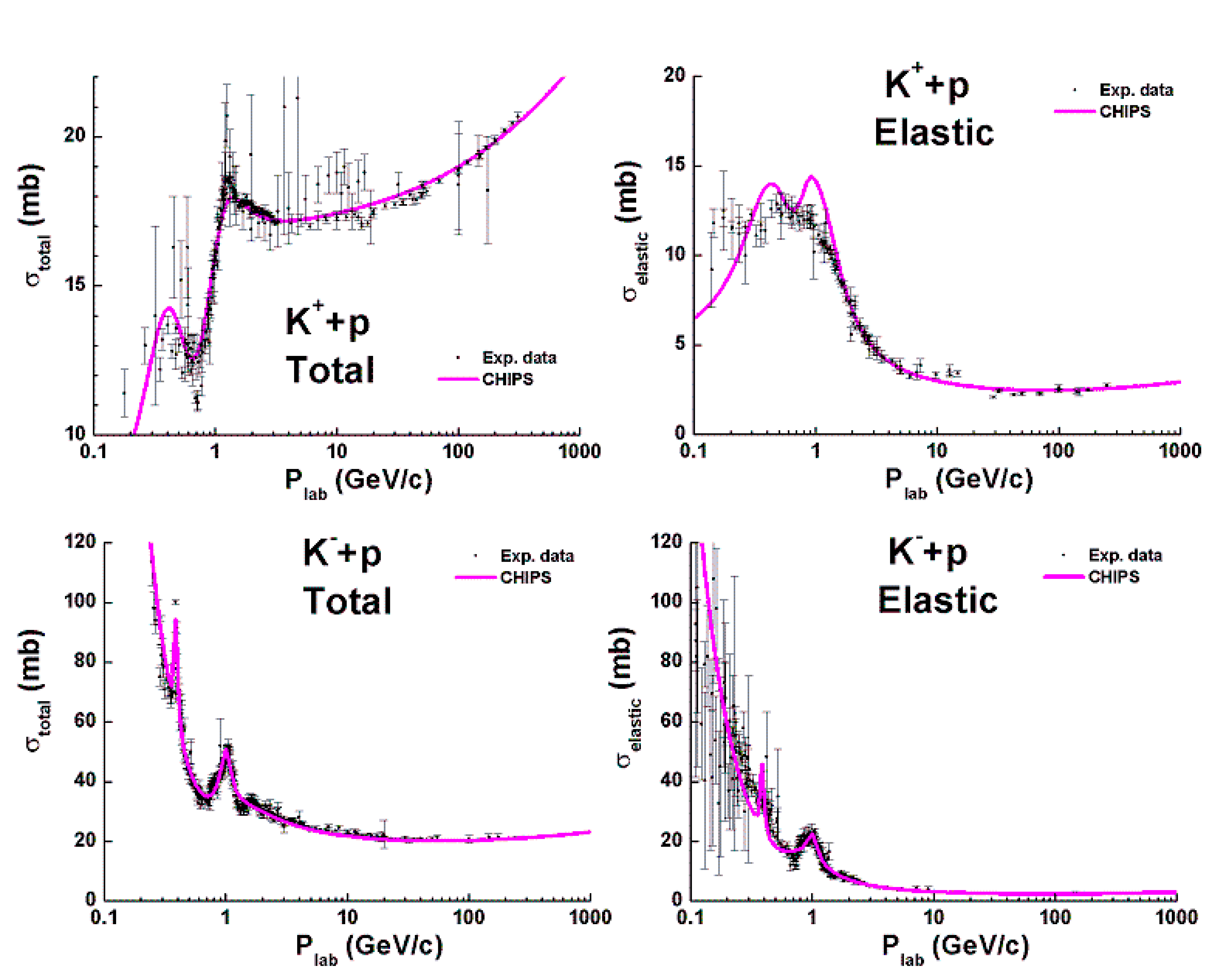
Fig. 81 Total and elastic cross sections of \(Kp\)-interactions. Points are experimental data from PDG data-base .

The reactions \(K^-+p\rightarrow \Sigma^-+\pi^+\) and \(K^-+p\rightarrow \Sigma^0+\pi^0\) can be explained by the annihilation of the \(u\)-antiquark of the \(K^-\) and the formation of \(s\)-channel resonances. The other reactions – \(K^-+p\rightarrow \Sigma^++\pi^-\) and \(K^-+p\rightarrow \Lambda+\pi^0\), are connected with quark exchange. As seen, the energy dependence of the cross sections of the two types of processes are different. The \(K^-+p\rightarrow n+K^0\) reaction must be caused by annihilation, but the dependence of its cross section on energy is closer to that of the quark exchange processes. The cross section of the reaction has a resonance structure only at \(P_{lab}<\) 2 GeV/c. Above that energy there is no structure. Because the cross section of the reaction is sufficiently small at high energies, one can omit its correct description.

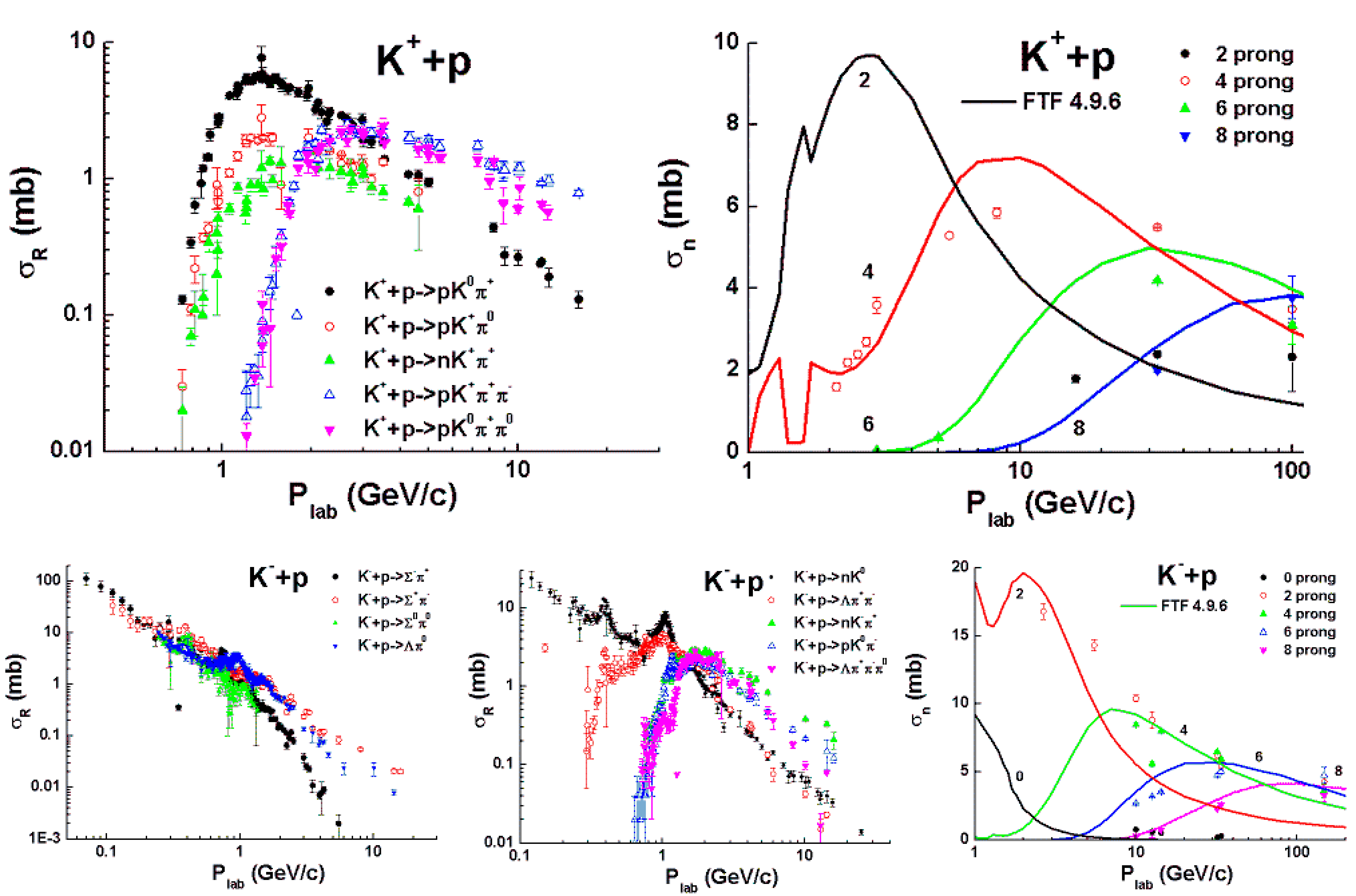
Fig. 82 Reaction cross sections of \(Kp\)-interactions. Points are experimental data .

\(K^-+p\rightarrow n+K^-+\pi^+\) and \(K^-+p\rightarrow p+K^0+\pi^-\) reactions are mainly caused by the diffraction dissociation of a projectile or a target hadron. The energy dependence of their cross sections are different from those of annihilation and quark exchange.

The same regularities can be seen in \(K^+p\) reactions. The energy dependence of the cross sections of the \(K^++p\rightarrow p+K^0+\pi^+\), \(K^++p\rightarrow p+K^++\pi^0\) and \(K^++p\rightarrow n+K^++\pi^+\) reactions are quite different from those of \(K^- + p\).

In summary, there are three types of energy dependence in the reaction cross sections. The rapidly decreasing one is due to annihilation. The cross sections of the quark exchange processes decrease more slowly. Finally, the diffraction cross sections grow with energy and reach near-constant values.

\(p \bar{p}\) interactions

Proton–antiproton interactions provide the beautiful possibility of studying annihilation processes in detail. The general properties of the interactions are presented in Fig. 83. Almost no structure is seen in the cross sections and their energy dependence is very different from the previously described reactions.

Fig. 83 General properties of \(\bar pp\)-interactions. Points are experimental data: data on total and elastic cross sections from PDG data-base [PDG12], other data from [eal73a][eal84].

Cross sections of the reactions – \(\bar p+p\rightarrow \pi^++\pi^-\) and \(\bar p+p\rightarrow K^++K^-\), decrease faster than other cross sections as a functions of energy. \(\bar p+p\rightarrow \pi^++\pi^-+\pi^0\) and \(\bar p+p\rightarrow 2\pi^++2\pi^-\) cross sections decrease less rapidly, nearly in the same manner as cross sections of the reactions – \(\bar p+p\rightarrow n+\bar n\) and \(\bar p+p\rightarrow \Lambda+\bar \Lambda\). The cross sections of the reaction – \(\bar p+p\rightarrow 2\pi^++2\pi^-+\pi^0\), is a slowly decreasing function. The cross section of the process – \(\bar p+p\rightarrow 3\pi^++3\pi^-+\pi^0\) varies only a little over the studied energy range. Cross sections of other reactions (\(\bar p+p\rightarrow p+\pi^0+\bar p\), \(\bar p+p\rightarrow p+\pi^++\pi^-+\bar p\) and so on) show behaviour typical of diffraction cross sections.

The main channel of \(\bar pp\) interactions at \(P_{lab}<\) 4 GeV/c is \(\bar p+p\rightarrow 2\pi^++2\pi^-+\pi^0\). At higher energies, there is a mixture of various channels. Such variety in the processes is indicative of complicated quark interactions. Possible quark flow diagrams are shown in Fig. 84.

Fig. 84 Quark flow diagrams of \(\bar pp\)-interactions.

As usual, quarks and antiquarks are shown by solid lines. Dashed lines present so-called string junctions. It is assumed that the gluon field in baryons has a non-trivial topology. This heterogeneity is called a “string junction”. Quark-gluon strings produced in the reaction are shown by wavy lines.

The diagram of Fig. 84a represents a process with a string junction annihilation and the creation of three strings. Diagram Fig. 84b describes quark-antiquark annihilation and string creation between the diquark and anti-diquark. Quark-antiquark and string junction annihilation is shown in Fig. 84c. Finally, one string is created in the process of Fig. 84e. Hadrons appear at the fragmentation of the strings in the same way that they appear in \(e^+e^-\)-annihilation. One can assume that excited strings with complicated gluonic field configurations are created in processes Fig. 84d and Fig. 84f. If the collision energy is sufficiently small glueballs can be formed in the process Fig. 84f. Mesons with constituent gluons or with hidden baryon number can be created in process Fig. 84d. Of course the standard FTF processes shown in the bottom of the figure are also allowed.

In the simplest approach it is assumed that the energy dependence of the cross sections of these processes vary inversely with a power of \(s\) as depicted in Fig. 84. Here \(s\) is center-of-mass energy squared. This is suggested by the reggeon phenomenology (at the leading order). Calculating the cross sections of binary reactions (in the reggeon framework, including higher-order terms) is a rather complicated procedure (see [KV94]) because there can be interactions in the initial and final states. Similar complications appear also in the computation of cross sections of other reactions [UG02].

Cross sections of hadron–nucleon processes

Total, elastic and inelastic hadron–nucleon cross sections

Parameterizations of the cross sections implemented in the CHIPS model of Geant4 (authors: M.V. Kossov and P.V. Degtyarenko) are used in the FTF model. The general form of the parameterization is:

\[\sigma = \sigma_{LE}+\sigma_{As}\]

where \(\sigma_{LE}\) is a low energy parameterization depending on the types of colliding particles, and \(\sigma_{As}\) is the asymptotic part of cross sections. The COMPLETE Collaboration proposed a hypothesis [ealCOMPLETEcollab02] that \(\sigma_{As}\) of total cross sections at very high energies does not depend on the types of colliding particles:

\[\sigma_{As}^{tot}= Z_{h_1h_2}+B\ \left( \log(s/s_0)\right)^2\]

\[\begin{split}B=0.3152, s_0 &=34.0 [(\mbox{GeV}/c)^2]\ \ \ (COMPLETE, 2002) \\ B=0.308~, s_0 &=28.9 [(\mbox{GeV}/c)^2]\ \ \ (PDG, 2006) \\ B=0.304~, s_0 &=33.1 [(\mbox{GeV}/c)^2]\ \ \ (\mbox{M. Ishida, K.Igi, 2009})\end{split}\]

while the pre-asymptotic part does depend on colliding particles (\(h_1\), \(h_2\)).

The CHIPS model \(\sigma_{As}\) for total and elastic cross sections has the same form:

\[\begin{split}\sigma_{As}= & \left\{A\ \left[\ln(P\_{lab}) - B\right]^2 + C + D/P_{lab}^{0.5} + E/P_{lab} + F/P_{lab}^2\right\}/ \\ &{} \left(1 + G/P_{lab}^{0.5} + H/P_{lab}^3 + I/P_{lab}^4\right)\ \ \ [\mbox{mb}]\end{split}\]

where \(P_{lab}\) is in [GeV/\(c\)], and the parameters \(A\), \(B\), etc. are given in the tables Table 44 and Table 45.

Table 44 CHIPS model parameters for total cross sections

\(h_1\ h_2\)	\(A\)	\(B\)	\(C\)	\(D\)	\(E\)	\(F\)	\(G\)	\(H\)	\(I\)
\(\pi^-p\)	0.3	3.5	22.3	12.0	0	0	0	0	0.4
\(\pi^+p\)	0.3	3.5	22.3	5.0	0	0	0	0	1.0
\(pp\)	0.3	3.5	38.2	0	0	0	0	0	0.54
\(np\)	0.3	3.5	38.2	0	0	52.7	0	0	2.72
\(K^+p\)	0.3	3.5	19.5	0	0	0	0.46	0	1.6
\(K^-p\)	0.3	3.5	19.5	0	0	0	-0.21	0	0.52
\(\bar pp\)	0.3	3.5	38.2	0	0	0	0	0	0

Table 45 CHIPS model parameters for elastic cross sections

\(h_1\ h_2\)	\(A\)	\(B\)	\(C\)	\(D\)	\(E\)	\(F\)	\(G\)	\(H\)	\(I\)
\(\pi^-p\)	0.0557	3.5	2.4	6.0	0	0	0	0	3.0
\(\pi^+p\)	0.0557	3.5	2.4	7.0	0	0	0	0	0.7
\(pp\)	0.0557	3.5	6.72	0	30.0	0	0	0.49	0.0
\(np\)	0.0557	3.5	6.72	0	32.6	0	0	0	1.0
\(K^+p\)	0.0557	3.5	2.23	0	0	0	-0.7	0	0.1
\(K^-p\)	0.0557	3.5	2.23	0	0	0	-0.7	0	0.075

The low energy parts of the cross sections are very different for various projectiles, and they are not presented here. These can be found in the corresponding classes of Geant4.

It is obvious that \(\sigma^{in}=\sigma^{tot}-\sigma^{el}\).

A comparison of the parameterizations with experimental data was presented in the previous figures.

Cross sections of quark exchange processes

Cross sections of quark exchange processes are parameterized as:

(235)\[\sigma_{qe}=\sigma_{in}\ A \ e^{-B\ y_{lab}}\]

where \(y_{lab}\) is a projectile rapidity in a target rest frame. \(A\) and \(B\) are parameters given in Table 48.

Table 48 Parameters of quark exchange cross sections

\(h_1\ h_2\)	\(A\)	\(B\)
\(pp/pn\)	1.85	0.7
\(\pi p/\pi n\)	240	2
\(Kp/Kn\)	40	2.25

The parameters were determined from a description of reaction channel cross sections.

Cross sections of antiproton processes

The annihilation cross section is parameterized as:

(236)\[\sigma_{ann}=\sigma_a\ +\ B\ X_b\ +\ C\ X_c\ +\ D\ X_d\]

where: \(X_i\) are the contributions of the diagrams of Fig. 84; all cross sections are given in \([mb]\);

(237)\[\begin{split}\sigma_a & = 25\ \sqrt{s}/\lambda^{1/2}(s,m^2_p,m^2_N) \\ \lambda(s,m^2_p,m^2_N) & = s^2+m_p^4+m_N^4-2sm_p^2-2sm_N^2-2m_p^2m_N^2 \\ X_b & = 3.13\ +\ 140\ (s_{th}-s)^{2.5}, \ \ \ s\ <\ s_{th} \\ X_b & = 6.8/\sqrt{s}, \ \ \ s\ >\ s_{th} \\ s_{th} &= (m_p+m_N+2m_\pi+\delta)^2 \\ X_c & = 2\ \frac{\sqrt{s}}{\lambda^{1/2}(s,m^2_p,m^2_N)}\frac{(m_p+m_N)^2}{s} \\ X_d & = 23.3/s\end{split}\]

Table 50 Coefficients B, C, and D.

	\(\bar pp\)	\(\bar pn\)	\(\bar np\)	\(\bar nn\)	\(\bar\Lambda p\)	\(\bar\Lambda n\)	\(\bar\Sigma^-p\)	\(\bar\Sigma^-n\)	\(\bar\Sigma^0p\)	\(\bar\Sigma^0n\)	\(\bar\Sigma^+ p\)	\(\bar\Sigma^+n\)
B	5	4	4	5	3	3	2	4	3	3	4	2
C	5	4	4	5	3	3	2	4	3	3	4	2
D	6	4	4	6	3	3	2	2	2	2	2	0

Table 51 Coefficients B, C, and D (continued).

	\(\bar\Xi^-p\)	\(\bar\Xi^-n\)	\(\bar\Xi^0p\)	\(\bar\Xi^0n\)	\(\bar\Omega^-p\)	\(\bar\Omega^-n\)
B	1	2	2	1	0	0
C	1	2	2	1	0	0
D	0	0	0	0	0	0

The coefficients \(B\), \(C\) and \(D\) are pure combinatorial coefficients calculated on the assumption that the same conditions apply to all quarks and antiquarks. For example, in \(\bar pp\) interactions there are five possibilities to annihilate a quark and an antiquark, and six possibilities to annihilate two quarks and two antiquarks. Thus, \(B=C=5\) and \(D=6\).

Note that final state particles in the process of Fig. 84b can coincide with initial state particles. Thus the true elastic cross section is not given by the experimental cross section.

At \(P_{lab}<\) 40 MeV/c antiproton-nucleon cross sections are:

\[\sigma^{tot}=1512.9,\ \ \sigma^{el}=473.2,\ \ \sigma_{a}=625.1,\ \ \sigma_{b}=0,\ \ \sigma_{c}=49.99,\ \ \sigma_{d}=6.61\]

All cross sections are given in mb. \(\sigma_{b}=0\) for \(\bar pp\)-interactions because the process \(\bar pp \rightarrow \bar nn\) is impossible at these energies (\(P_{lab}<\) 40 MeV/c).

Cross sections of diffractive and non-diffractive processes

As mentioned above, three processes are considered in the FTF model at high energies: projectile diffraction (pd), target diffraction (td) and non-diffractive interactions (nd). They are parameterized as:

(238)\[\begin{split}\sigma^{pd}_{pp} &= \sigma^{td}_{pp}=6\ +\ \sigma^{in}\frac{1.5}{s} \ \ \ (\mbox{mb}) \\ \sigma^{pd}_{\bar pp} &= \sigma^{td}_{\bar pp}=6\ +\ \sigma^{in}\frac{1.5}{s} \ \ \ (\mbox{mb}) \\ \sigma^{pd}_{\pi p} &= 6.2\ -\ e^{-\frac{(\sqrt{s}-7)^2}{16}} \\ \sigma^{td}_{\pi p} &= 2 + 22/s \ \ \ (\mbox{mb}) \\ \sigma^{pd}_{Kp} &=4.7, \\ \sigma^{td}_{Kp} &=1.5 \ \ \ (\mbox{mb})\end{split}\]

For the determination of these cross sections, inclusive spectra of particles in hadronic interactions were used. In Fig. 85 an inclusive spectrum of protons in the reaction \(p+p\rightarrow p+X\) is shown in comparison with model predictions.

Fig. 85 Left: inclusive spectrum of proton in \(pp\)-interactions at \(P_{lab}=24\) GeV/c. Points are experimental data [eal74], lines are model calculations. Right: single diffraction dissociation cross section in \(pp\)-interactions. Points are data gathered by K. Goulianos and J. Montanha [GM99]. Lines are FTF model calculations.

As it can be seen, all the models have difficulties in describing the data. In the FTF model this was overcome by tuning the single diffraction dissociation cross section. Tuning was possible by the fact that the height of the proton peak at large rapidities depends on this cross section (see left Fig. 85).

The \(2\sigma^{pd}_{pp}\) (the factor of 2 is due to the fact that \(\sigma^{pd}_{pp} = \sigma^{td}_{pp}\)) predicted by the expression (blue solid curve) is shown at the right of Fig. 85 in a comparison with experimental data gathered by K. Goulianos and J. Montanha [GM99]. The values are larger than experimental data. Though taking into account the restriction that the mass of a produced system, \(X\), cannot be very small or very large (\(M^2/s<\) 0.05 and \(M>\) 1.5 GeV) brings the predictions closer to the data. So, the accounting of this restriction is very important for a correct reproduction of the data.

A more complicated situation arises with \(\pi p\)- and \(Kp\)-interactions. The set of experimental data on diffraction cross sections is very restricted. Thus, a refined tuning was used. The FTF processes discussed above contribute in various regions of particle spectra. The target diffraction dissociation, \(\pi+p\rightarrow \pi+X\), gives its main contribution at large values of \(x_F=2p_z/\sqrt{s}\) for \(\pi\)-mesons. The projectile diffraction dissociation contribution (\(\pi+p\rightarrow X+p\)) has a maximum at \(x_F\sim -1\). Thus, using various experimental data and varying the cross sections of the processes, the points presented in the lower left corner of Fig. 86 were obtained. They were parameterized by the expressions in (238). A correct reproduction of particle spectra in the central region, \(x_F\sim\) 0, was very important for these. As a result, we have a good description of \(\pi\)-meson spectra in the interactions at various energies.

In \(Kp\)-interactions the projectile diffraction cross sections were determined by tuning on proton spectra from the reactions \(K+p\rightarrow p+X\) (see Fig. 87). There are no data on leading \(K\)-meson spectra in the reactions \(K+p\rightarrow K+X\). Thus, \(\pi^-\)-meson spectra in the central region were tuned. At a given value of a projectile diffraction cross section, the central spectrum depends on a target diffraction. This was used to determine the target diffraction cross sections. The estimated cross sections are shown in the lower left corner of Fig. 87. As a result, a satisfactory description of meson spectra was obtained.

Fig. 86 Upper figures: inclusive spectra of protons and \(\pi^+\)-mesons in \(\pi^+p\)-interactions. Points are experimental data [eal73b]. Lines represent the contributions of the various FTF processes calculated by assuming that the probability of each process is 100 %. Bottom left figure: diffraction dissociation cross sections obtained by tuning (points), and their description (lines) by the expression for \(\pi\) in (238). Bottom right figure: rapidity spectrum of \(\pi^+\)-mesons in \(\pi^+p\)-interactions at \(p_{lab}=\)100 GeV/c. Points are experimental data [Whi74].

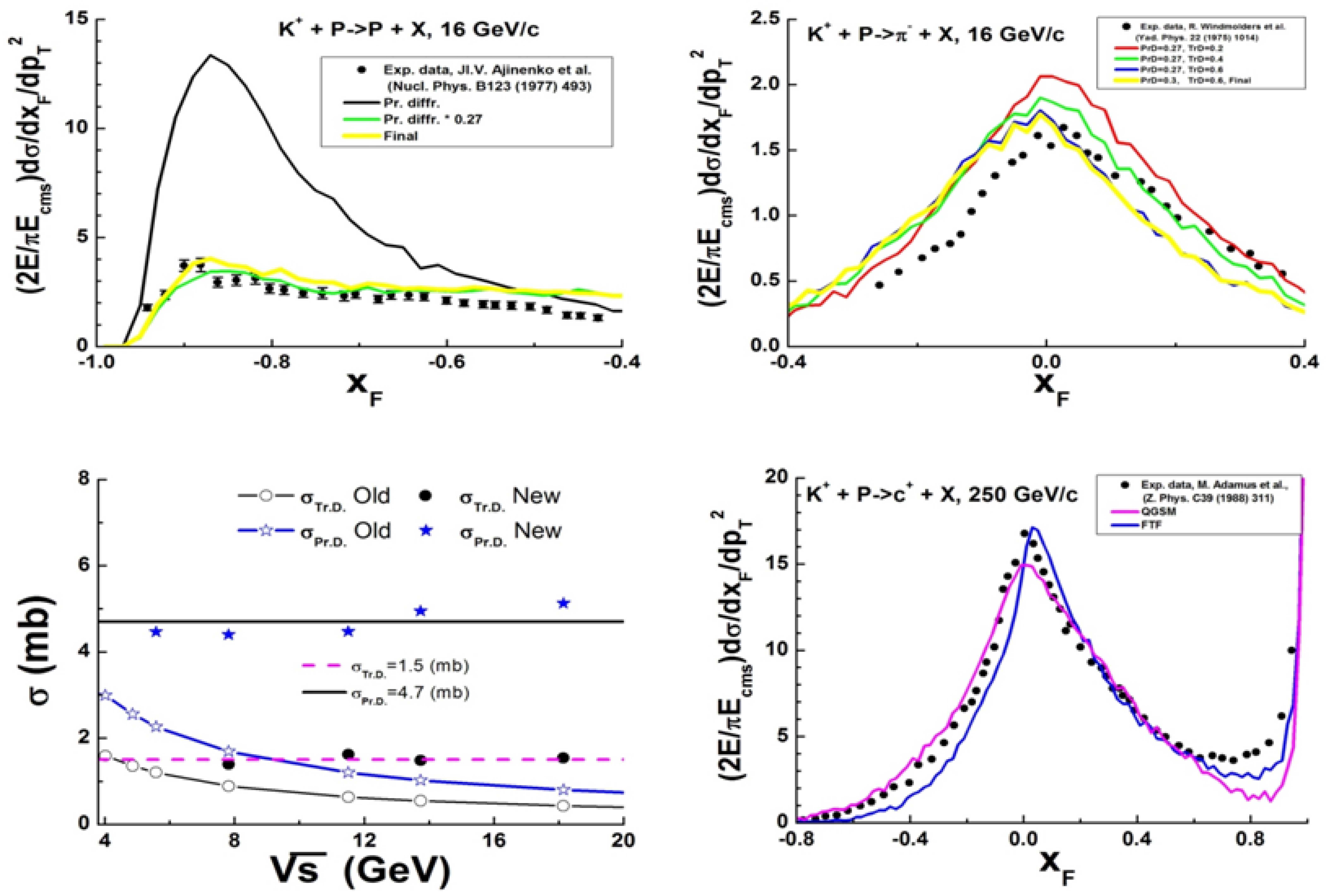
Fig. 87 Upper figures: inclusive spectra of protons and \(\pi^-\)-mesons in :math:`(Kp)`-interactions. Points are experimental data [eal86][eal77]. Lines are FTF calculations. Bottom left figure: diffraction dissociation cross sections obtained by tuning (points), and their description (lines) by the expression for Kp in (238). Bottom right figure: \(x_F\) spectrum of positive charged particles in \(Kp\)-interactions at \(p_{lab}=\)250 GeV/c. Points are experimental data [Whi74], lines are model calculations.

Simulation of hadron-nucleon interactions

Simulation of meson–nucleon and nucleon–nucleon interactions

Colliding hadrons may either be on or off the mass shell when they are bound in nuclei. When they are off-shell the total mass of the hadrons is checked. If the sum of the masses is above the center-of-mass energy of the collision, the simulated event is rejected. If below, the event is accepted. It is assumed that due to the interaction the hadrons go on-shell, and the center-of-mass energy of the collision is not changed.

The simulation of an inelastic hadron-nucleon interaction starts with a choice: should a quark exchange or a diffractive/non-diffractive excitation be simulated? The probability of a quark exchange is given by \(W_{qe}=\sigma_{qe}/\sigma^{in}\). The combined probability of diffractive dissociation and non-diffractive excitation is then \(1-W_{qe}\). \(\sigma_{qe}\) depends on the energies and flavors of the colliding hadron (see Eq.(235)).

If a quark exchange is sampled, the quark contents of the projectile and target are determined. After that the possibility of a quark exchange is checked. A meson consists of a quark and an antiquark. Thus there is no alternative but to choose a quark. Let it be \(q_M\). A baryon has three quarks, \(q_1\), \(q_2\) and \(q_3\). The quark from the meson can be exchanged, in principle, with any of the baryon quarks, but the above description of the experimental data indicates that an exchange of quarks with the same flavor must be suppressed. So, only the exchange of quarks with different flavors is allowed. After the exchange (\(q_M \leftrightarrow q_i\)), the new contents of the meson and the baryon are determined. The new meson may be either pseudo-scalar or pseudo-vector with a 50% probability. The new baryon may be in its ground state, or in an excited state. The probability of an excited baryon state is assumed (as common also in other codes) to be 0.5 for both \(\pi N\)-interactions and \(KN\)-interactions. Only \(\Delta(1232)\)’s are considered as excited states. If all quarks of a baryon have the same flavor, the \(\Delta(1232)\) is always created (\(\Delta(1232)^{++}\) or \(\Delta(1232)^{--}\)).

The same procedure is followed for a projectile baryon, but in this case any quark of the projectile or target may participate in an exchange if they have different flavors. Only the ground state of the new baryon is considered.

In order to generate a transverse momentum between the two final-state hadrons, these final-state hadrons undergo to either an additional elastic scattering with probability \(W_{el}=2.256\ e^{-0.6\ y_{lab}}\) (the parameters have been fitted from experimental data), or a diffractive/non-diffractive excitation with probability \(1-W_{el}\), where \(y_{lab}\) is the rapidity of the projectile in the target rest frame.

The above procedure is sufficient for a description of hadron-nucleon reaction cross sections at \(p_{lab}<\) 3 – 5 GeV/c. At higher energies, diffractive dissociations and non-diffractive excitations must be simulated.

As mentioned above, there can be a projectile diffraction, or a target diffraction, or a non-diffractive interaction. Probabilities of the corresponding processes at high energies are: \(\sigma^{pd}/\sigma^{in}\), \(\sigma^{td}/\sigma^{in}\), and \((\sigma^{in}-\sigma^{pd}-\sigma^{td})/\sigma^{in}\). The processes are sampled randomly.

Having sampled a projectile diffraction or a target diffraction, the corresponding light-cone momentum (\(P^-\) or \(P^+\)) is chosen according to the distribution: \(dP^-/P^-\) or \(dP^+/P^+\). Boundaries for a sampling have to be determined before.

Let us consider the kinematics of projectile diffraction, \(P+T\rightarrow P'+T\), for the definition of these boundaries. It is obvious that a mass of the diffractive produced system, \(m_{P'}\), must satisfy the conditions:

\[m_D \leq m_{P'} \leq \sqrt{s} -m_T\]

where \(m_D\) is the minimal mass of the system, \(s\) is the center-of-mass energy squared, \(m_T\) is the mass of the target. If there is not a transverse momentum transfer, and \(m_{P'}\) reaches the lower boundary then

\[P^-_{min}=\sqrt{m_D^2+p_z^2}-p_z , \ \ \ p_z=\lambda^{1/2}(s,m_D^2,m_T^2)/2\sqrt{s}\]

(See (237) for the definition of \(\lambda()\).)

When \(m_{P'}\) reaches the upper boundary, the longitudinal momenta of the particles are zeros. Thus,

\[P^-_{max}=\sqrt{s}-m_T\]

Having sampled \(P^-\), then \(m_{P'}\) and \(P^+\) can be found with the help of the energy-momentum conservation law written is the center-of-mass system:

\[\begin{split}\left\{ \begin{array}{l}E_{P'}+E_T=\sqrt{s}\\ P_{z,P'}+P_{z,T}=0 \end{array} \right. \left| \begin{array}{l}P^-_{P'}+P^-_T=\sqrt{s}\\ P^+_{P'}+P^+_{T}=\sqrt{s} \end{array} \right. \left| \begin{array}{l}P^-_T=\sqrt{s}- P^-_{P'}\\ P^+_T=m_T^2/P^-_T \\ m_{P'}^2=P^-_{P'}\cdot (\sqrt{s}-P^+_T) \end{array} \right.\end{split}\]

The transferred transverse momentum is sampled according to the distribution:

\[dW=\frac{1}{\pi \langle P^2_\perp \rangle }\ e^{-P^2_\perp/\langle P^2_\perp \rangle}d^2P_\perp, \ \ \ \langle P^2_\perp \rangle =0.3\ (\mbox{GeV}/c)^2\]

To account for it, it is enough to replace the masses with the transverse masses, \(m_\perp=\sqrt{m^2+P^2_\perp}\).

The light-cone momenta transferred to the projectile are:

\[Q^+=P^+_{T,0}-P^+_{T}, \ \ \ Q^-=P^-_{T,0}-P^-_{T}\]

where \(P^+_{T,0}\) and \(P^-_{T,0}\) are the light-cone momenta of the target in the initial state.

In the case of non-diffractive excitation (\(P+T\rightarrow P'+T'\)), \(P^-_{P'}\) is sampled first of all as it was described above at \(m_T=m_{T,nd}\), where \(m_{T,nd}\) is the minimal mass of a target-originated particle produced in the non-diffractive excitation. After that, \(P^+_{T'}\) is independently sampled at \(m_P=m_{P,nd}\). The minimal light-cone momenta, \(P^-_{P'}\) and \(P^+_{T'}\), are calculated at \(m_P=m_{P,nd}\) and \(m_T=m_{T,nd}\). At the last step it is checked that \(m_{P'} \geq m_{P,nd}\) and \(m_{T'} \geq m_{T,nd}\). In the current version of the FTF model the same values for minimal masses are used in the diffractive and non-diffractive excitation.

Table 54 Minimal masses of diffractive produced strings

	\(p/n\)	\(\pi\)	\(K\)
\(m_D\) (MeV)	1160	500	600

Simulation of antibaryon–nucleon interactions

At the beginning of the simulation of an annihilation interaction, the cross sections of the processes (see Fig. 84) are calculated (see (236)). After that a sampling of the processes takes place.

In the cases of the processes Fig. 84b and Fig. 84e quarks for the annihilation are chosen randomly. In each of the processes only one string is created. Its mass is equal to the center-of-mass energy of the interaction. After that the string is fragmented. It is required that in the fragmentation of the process Fig. 84b there must not be a baryon and an antibaryon in the final state.

At sufficiently high energies the standard FTF processes can be simulated as it was described above.

In the process Fig. 84c only 2 strings will be created. If their masses are given, the kinematical properties of the strings can be determined with the help of the energy-momentum conservation law. The masses must be related to the momenta of the quarks and antiquarks.

We assume that in the process all quarks and antiquarks are in the same conditions, thus, their transverse momenta are sampled independently according to the gaussian distribution with \(\langle P_\perp^2 \rangle=0.04\) \((\mbox{GeV}/c)^2\). To guarantee that the sum of the transverse momenta is zero, the transverse momentum of each particle is re-defined as follows: \(\vec P_{\perp i} \rightarrow \vec P_{\perp i} - \frac{1}{4}\sum_{j=1}^{4}\vec P_{\perp j}\).

To find the longitudinal momenta of quarks we use the light-cone momenta: total light-cone momenta of projectile-originated antiquarks and target-originated quarks,

\[P^+=P^+_{\bar q_1}+P^+_{\bar q_2}, \ \ \ P^-=P^-_{q_1}+P^-_{q_2}\]

Let us introduce also the light-cone momentum fractions:

\[\begin{split}x^+_{\bar q_1} &= P^+_{\bar q_1}/P^+, \ \ \ x^+_{\bar q_2}=1-x^+_{\bar q_1} \\ x^-_{q_1} &= P^-_{q_1}/P^-, \ \ \ x^-_{q_2} =1-x^-_{q_1}\end{split}\]

Using these variables, the energy-momentum conservation law in the center-of-mass system can be written as:

\[\begin{split}\frac{P^+}{2} + \frac{\alpha}{2 \ P^+} \ + \ \frac{P^-}{2} + \frac{\beta}{2 \ P^-} &= \sqrt{s} \\ \frac{P^+}{2} - \frac{\alpha}{2 \ P^+} \ - \ \frac{P^-}{2} + \frac{\beta}{2 \ P^-} &= 0\end{split}\]

\[\begin{split}\alpha &=\frac{m_{\perp \bar q_1}^2}{x^+_{\bar q_1}}+\frac{m_{\perp \bar q_2}^2}{1-x^+_{\bar q_1}} \\ \beta &=\frac{m_{\perp q_1}^2}{x^-_{ q_1}}+\frac{m_{\perp q_2}^2}{1-x^-_{ q_1}}\end{split}\]

A solution of the equations at \(\sqrt{\alpha}+\sqrt{\beta}\ \leq \ \sqrt{s}\) is:

\[\begin{split}P^+ &= \frac{s + \alpha - \beta + \lambda^{1/2}(s,\alpha,\beta)}{2\ \sqrt{s}} \\ P^- &= \frac{s - \alpha + \beta + \lambda^{1/2}(s,\alpha,\beta)}{2\ \sqrt{s}}\end{split}\]

(See (237) for the definition of \(\lambda()\).)

If \(\sqrt{\alpha}+\sqrt{\beta}\ > \ \sqrt{s}\), the transverse momenta and \(x\)s are re-sampled until the inequality is broken.

Because quarks are in the same conditions, the distribution on \(x\) can have the form \(x^a\ (1-x)^a\). A recommended value of \(a\) can be zero or \(-0.5\). We chose \(a=-0.5\). We assumed also that the quark masses are zero. Probably, other values could be used, but we have not yet found experimental data sensitive to these parameters.

For the simulation of the process Fig. 84a we follow the same approach, and introduce light-cone momentum fractions – \(x^+_{\bar q1},\ x^+_{\bar q2},\ x^+_{\bar q3}\) and \(x^-_{q_1},\ x^-_{q_2},\ x^-_{q_3}\). The distribution on \(x\)s is chosen according to the form:

\[dW\propto x^a_{q_1}\ x^a_{q_2}\ x^a_{q_3}\delta(1-x_{q_1}-x_{q_2}-x_{q_3})dx_{q_1}\ dx_{q_2}\ dx_{q_3}, \ \ \ a=-0.5\]

It is obvious that in this case:

\[\alpha=\sum_{i=1}^3\frac{m_{\perp \bar q_i}^2}{x^+_{\bar q_i}} \ ,\ \ \ \ \beta =\sum_{i=1}^3\frac{m_{\perp q_i}^2}{x^-_{ q_i}}\]

Flowchart of the FTF model

The simulation of hadron-nucleus or nucleus-nucleus interaction events starts with an initialization (done “on-the-fly” just before simulating the interaction, not at the beginning of the program) of the model variables: calculations of cross sections, setting up slopes, masses and so on. The next step is the determination of intra-nuclear collision multiplicity with the help of Glauber model. If the energy of collisions is sufficiently high, the simulation of secondary particle cascading within the reggeon theory inspired model (RTIM [AWU97][AWU98]) is carried out. After that all involved nuclear nucleons are put on the mass-shell. If the energy is not high enough these steps are skipped. The reason for this will be explained later.

The main job of the FTF algorithm is done in the loop over intra-nuclear collisions. At that moment, the time ordering of the collisions has been determined. For each collision, it is sampled what has to be simulated – elastic scattering, inelastic interaction or annihilation for projectile antibaryons. For each branch, an adjustment of the participating nuclear nucleon is performed at low energy, and the corresponding process is simulated. In the case of the sampling of the inelastic interaction at high energy there is an alternative – to reject the interaction or to process it.

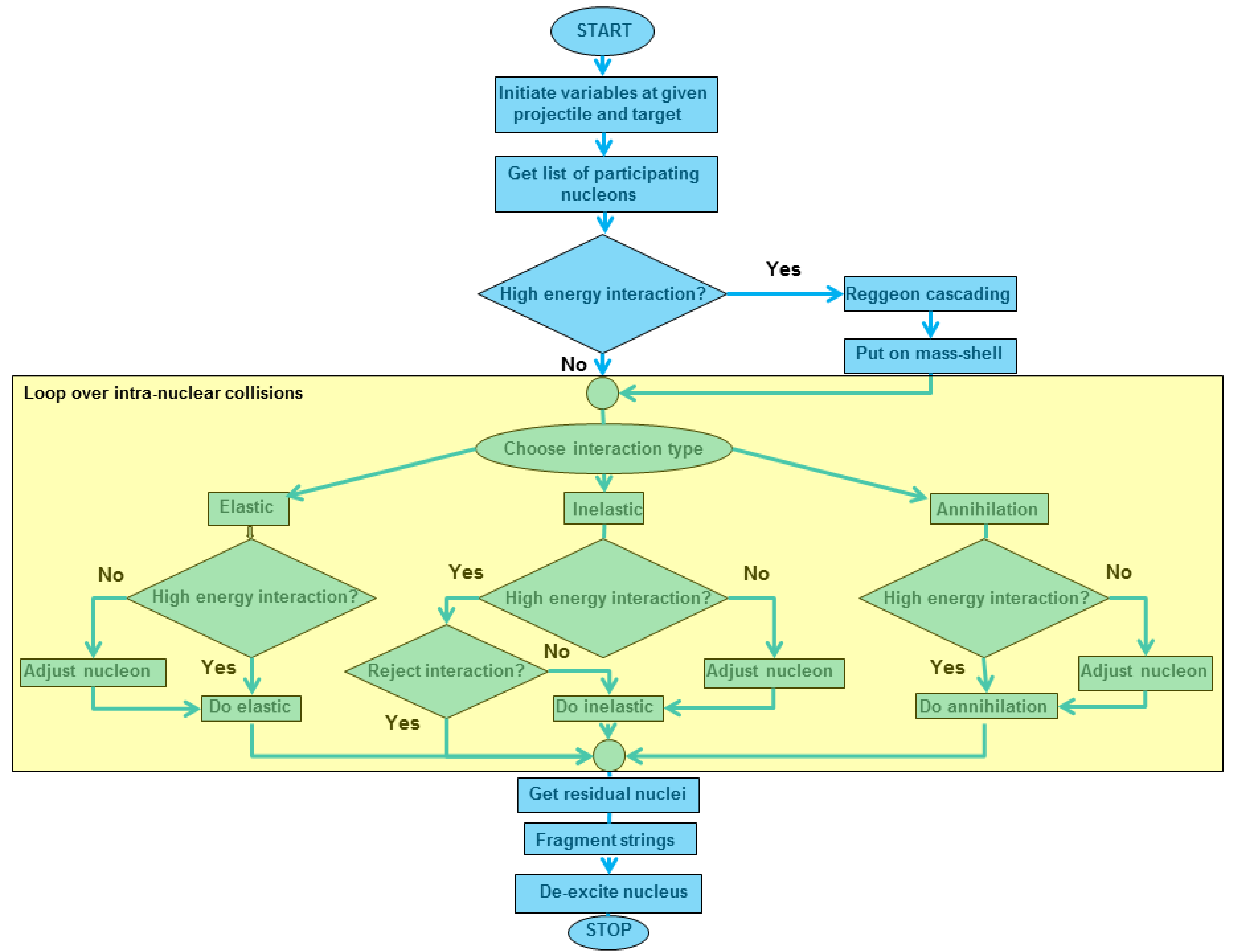
Fig. 88 Flowchart of the FTF model.

At the end of the loop, the properties of nuclear residuals (mass number, charge, excitation energy and 4-momentum) are transferred to a calling program. The program initiates the fragmentation of created strings and decays the excited residuals.

Simulations of elastic scattering, inelastic interactions and annihilation were considered above. Other steps of the FTF model will be presented below.

Simulation of nuclear interactions

Sampling of intra-nuclear collisions

Classical cascade-type sampling

As it is known, the intra-nuclear cascade models like the ones implemented in Geant4 – The Bertini Intranuclear Cascade Model, The Binary Cascade Model, INCL++: the Liège Intranuclear Cascade Model – work well for projectile energies below 5 – 10 GeV. The first step in these models is the sampling of the impact parameter, \(b\). The next step is the sampling of a point where the projectile will interact with nuclear matter (see Fig. 89a).

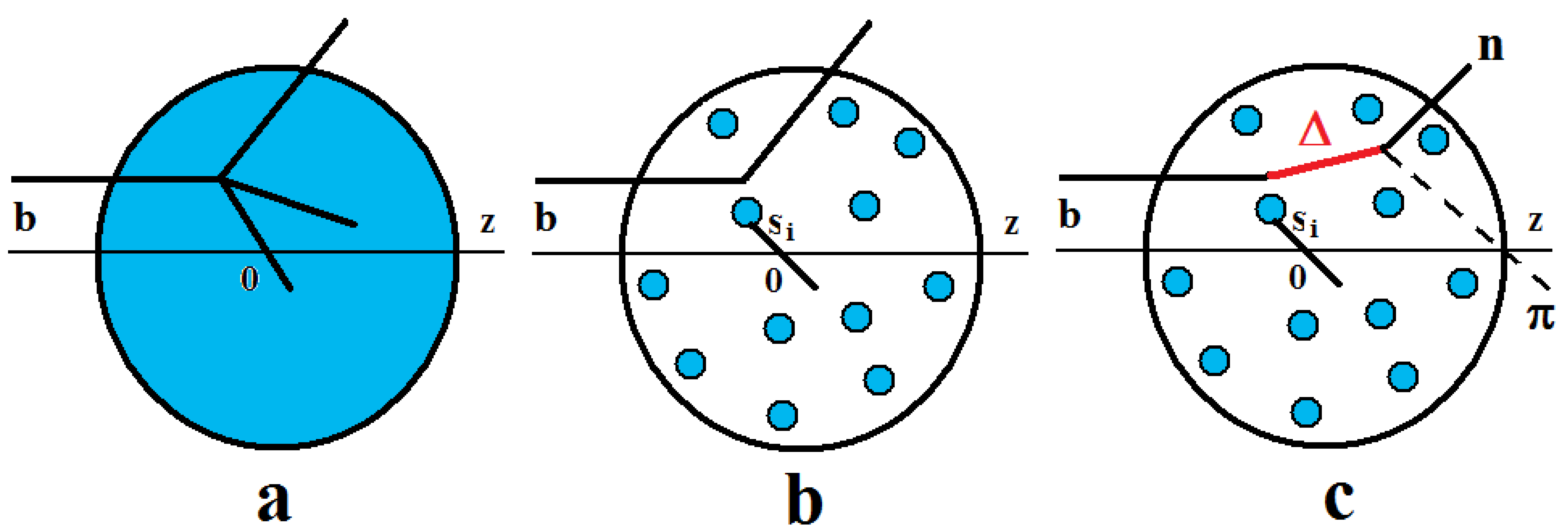
Fig. 89 Cascade-type sampling.

The following consideration is used here: the probability that the projectile reaches a point \(z\) going from minus infinity to the point \(z\) is

\[P = e^{-\sigma^{tot} \int_{-\infty}^z\rho_A(\vec b,z')\ dz'}\]

where \(\sigma^{tot}\) is the total cross section of the projectile-nucleon interaction, \(\rho_A\) is the density of the nucleus considered as a continuous medium.

The probability that the projectile will have an interaction in the range \(z\) – \(z+dz\) is equal to \(\sigma^{tot} \rho_A(\vec b,z)\ dz\). Thus, the total probability is:

\[\begin{split}P(\vec b,z) &= \sigma^{tot} \rho_A(\vec b,z)\ e^{-\sigma^{tot} \int_{-\infty}^z\rho_A(\vec b,z')\ dz'}\ dz \\ P(\vec b) &= \int_{-\infty}^{+\infty}P(\vec b,z)\ dz=1- e^{-\sigma^{tot} \int_{-\infty}^\infty\rho_A(\vec b,z')\ dz'}\end{split}\]

Having sampled the interaction point, the choice between an elastic scattering and an inelastic interaction is then implemented.

In the case of the inelastic interaction, a multi-particle production process is simulated. After this, for each produced particle new interaction points are sampled, and so on.

In the case of the elastic scattering, the scattering is simulated, and then new interaction points for the recoil nucleon and the projectile are sampled.

The prescription is changed a little bit by replacing the continuous medium with a collection of \(A\) nucleons located in the points \(\{\vec s_i,z_i\}\), \(i=1\)–\(A\) where \(\{\vec s_i\}\) are coordinates of the nucleons in the impact parameter plane. The projectile can interact with the nearest nuclear nucleon, whose \(\vec s_i\) satisfies the condition: \(|\vec b -\vec s_i| \leq \sqrt{\sigma^{tot}/\pi}\) (see Fig. 89b).

In the first versions of the cascade models, only nucleons and pions were considered. When it was recognized that most of inelastic reactions at intermediate energies are going through resonance productions, various baryonic and mesonic resonances were included, and the algorithm changed (see Fig. 89c). As energy grows, more and more heavy resonances are produced. Because the properties of resonance-nucleon collisions were not known, the interpretation of the Glauber approximation was very useful.

Short review of Glauber approximation

The Glauber approach [Gla59][Gla67] was proposed in the framework of the potential theory, before the creation of the intra-nuclear cascade models. Its main assumption is that at sufficiently high energies many partial waves contribute to a particle elastic scattering amplitude, \(f(\vec q)\). Thus, a summation on angular momenta can be replaced by an integral:

\[f(\vec q)=\frac{iP}{2\pi}\int e^{i\vec q \vec b}\left[ 1-e^{i\chi(\vec b)}\right]\ d^2b \ ,\ \ \ \frac{d\sigma}{d\Omega}=|f(\vec q)|^2\]

\[\gamma(\vec b)=\frac{1}{2\pi i P}\int e^{-i\vec q \vec b}\ f(\vec q)\ d^2q\]

where \(P\) is the projectile momentum, \(q\) is the transferred transverse momentum, \(\vec b\) is the impact parameter, \(\chi\) is the phase shift, and \(\gamma\) is the scattering amplitude in the impact parameter representation.

Due to the additivity of potentials, it was natural to assume that the overall phase shift for the projectile scattered on \(A\) centers located in the points \(\{\vec s_i,z_i\}\), \(i=1\)–\(A\) is the sum of the corresponding shifts on each center:

\[\chi_{hA}=\sum_{i=1}^A \chi(\vec b-\vec s_i)\]

(239)\[\gamma_{hA}(\vec b)=1-\prod_{i=1}^A\left[ 1-\gamma(\vec b-\vec s_i)\right]\]

Because the positions of nucleons in nuclei are not fixed, the Eq. (239) has to be averaged, and the hadron-nucleus scattering amplitude takes the form:

\[F^{hA}_{0\rightarrow f}=\frac{iP}{2\pi} \int d^2b\ e^{-i\vec q \vec b} \ \left\{1-\prod_{i=1}^A\left[ 1-\gamma(\vec b-\vec s_i)\right]\right\}\ \Psi_0(\{r_A\})\Psi_f^*(\{r_A\})\prod_{i=1}^A d^3r_i\]

where \(\Psi_0\) and \(\Psi_f\) are wave functions of the nucleus in initial and final states, respectively.

In the case of elastic scattering, \(\Psi_0=\Psi_f\), we have:

(240)\[\begin{split}F^{hA}_{el} &=\frac{iP}{2\pi} \int d^2b\ e^{-i\vec q \vec b} \ \left\{1- \prod_{i=1}^A\left[ 1-\int \gamma(\vec b-\vec s_i)\rho_A(\vec s_i,z')d^2s_idz'\right]\right\} \\ & \simeq \frac{iP}{2\pi} \int d^2b\ e^{-i\vec q \vec b} \ \left\{1-\left[ 1-\frac{1}{A}\int \gamma(\vec b-\vec s)T_A(\vec s)d^2s\right]^A\right\} \\ & \simeq \frac{iP}{2\pi} \int d^2b\ e^{-i\vec q \vec b} \ \left\{1-e^{-\int \gamma(\vec b-\vec s)T_A(\vec s)d^2s}\right\} \\ & \simeq \frac{iP}{2\pi} \int d^2b\ e^{-i\vec q \vec b} \ \left\{1-e^{-\sigma_{hN}^{tot}(1-i\alpha)T_A(\vec b)/2}\right\}\end{split}\]

Some assumptions and simplifications have been used in the above derivations. First of all, it was assumed that \(|\Psi_0|^2\simeq\prod_{i=1}^A\rho(\vec s_i,z_i)\) where \(\rho\) is the one-particle nuclear density. Because the nucleon coordinates must obey the obvious condition: \(\sum_{i=1}^A \vec r_i=0\), it would be better to use \(|\Psi_0|^2\simeq \delta(\sum_{i=1}^A \vec r_i)\prod_{i=1}^A\rho(\vec s_i,z_i)\). Considering this \(\delta\)-function corresponds to take into account the center-of-mass correlation. The second assumption is that \(A\) is sufficiently large, thus \((1-\frac{x}{A})^A_{A\rightarrow \infty}=e^{-x}\) (optical limit). A thickness function of the nucleus was introduced:

\[T(\vec b)=A\int^{+\infty}_{-\infty}\rho(\vec b,z)\ dz\]

It was assumed also that the range of the \(\gamma\)-function is much less than the range of the nuclear density: \(\int \gamma(\vec b-\vec s)T_A(\vec s)d^2s\simeq \sigma_{hN}^{tot}(1-i\alpha)T_A(\vec b)/2\), where \(\sigma_{hN}^{tot}\) is the hadron-nucleon total cross section, and \(\alpha=Re\ f(0)/Im \ f(0)\) is the ratio of real and imaginary parts of hadron-nucleon elastic scattering amplitude at zero momentum transfer.

There were many applications of the Glauber approach for calculations of elastic scattering cross sections, cross sections of nuclear excitations, coherent particle production and so on. We consider here only its application to inelastic reactions.

If the energy resolution of a scattered projectile is not too high, many nuclear excited states can contribute to the scattering amplitude: \(F^{hA}=\sum_f F^{hA}_{0\rightarrow f}\). To find the corresponding cross section, it is usually assumed that a set of final-state wave functions satisfy the completeness relation: \(\sum_f \Psi_f(\{\vec r_i\}) \Psi^*_f(\{\vec r_j'\})=\prod_{i=1}^A\delta(\vec r_i-\vec r_i')\).

In the Glauber approach, it is possible to show that the cross section of elastic and quasi-elastic scatterings has the following expression:

\[\sigma^{hA}_{el.+qel.}=\int d^2b\ \left\{1-2Re\ e^{-\sigma_{hN}^{tot}(1-i\alpha)T_A(\vec b)/2}+e^{-\sigma_{hN}^{in}T_A(\vec b)}\right\}\]

Subtracting from it the cross section of the elastic scattering, we have:

\[\begin{split}\sigma^{hA}_{qel.} & = \int d^2b\ \left\{e^{-\sigma_{hN}^{in}T_A(\vec b)}-e^{-\sigma_{hN}^{tot}T_A(\vec b)}\right\} \\ &= \int d^2b\ e^{-\sigma_{hN}^{tot}T_A(\vec b)}\left\{e^{\sigma_{hN}^{el}T_A(\vec b)}-1\right\} \\ & = \int d^2b\ e^{-\sigma_{hN}^{tot}T_A(\vec b)}\sum_{n=1}^\infty\frac{[\sigma_{hN}^{el}T_A(\vec b)]^n}{n!}\end{split}\]

The last expression shows that the quasi-elastic cross section is a sum of cross sections with various multiplicities of elastic scatterings. It coincides with the prescription of the cascade model if only elastic scatterings of the projectile are considered.

The cross section of multi-particle production processes in the Glauber approach has the form:

(241)\[\begin{split}\sigma^{hA}_{mpp} & = \sigma^{hA}_{tot}-\sigma^{hA}_{el.+qel.} =\int d^2b\ \left\{1-e^{-\sigma_{hN}^{in}T_A(\vec b)}\right\} \\ & = \int d^2b\ e^{-\sigma_{hN}^{in}T_A(\vec b)}\sum_{n=1}^\infty\frac{[\sigma_{hN}^{in}T_A(\vec b)]^n}{n!}\end{split}\]

This expression coincides with the analogous cascade expression in the case of a projectile particle that can be distinguished from the produced particles. Of course, it cannot be so in the case of projectile pions.

In the FTF model of Geant4 it is assumed that projectile- and target-originated strings are distinguished. Thus, the cascade-type algorithm of the sampling of the multiplicities and types of interactions in nuclei is used.

A generalization of the Glauber approach for the case of nucleus-nucleus interactions was proposed by V. Franco [Fra68]. In this approach, the cross section of multi-particle production processes is given by the expression:

(242)\[\sigma^{AB}_{mpp} = \int d^2b\ \left\{1-\prod_{i=1}^A\prod_{j=1}^B \left[ 1-g(\vec b+\tau_j-\vec s_i)\right]\right\}\cdot |\Psi_0^A(\{r_A\})|^2|\Psi_0^B(\{t_B\})|^2\left[\prod_{i=1}^A d^3r_i\right]\left[\prod_{j=1}^B d^3t_i\right]\]

where \(g(\vec b)=\gamma(\vec b)+\gamma^*(\vec b)- |\gamma(\vec b)|^2\), \(A\) and \(B\) are mass numbers of colliding nuclei, \(\{\vec \tau_j\}\) is a set of impact coordinates of projectile nucleons (\(\vec t=(\vec \tau, z)\)).

Considering \(g(\vec b)\) as a probability that two nucleons separated by the impact parameter \(\vec b\) will have an inelastic interaction, a simple interpretation of the Eq. (242) can be given. The expression in the curly brackets of Eq. (242) is the probability that there will be at least one or more inelastic nucleon-nucleon interactions. \(|\Psi_0^A(\{r_A\})|^2\ |\Psi_0^B(\{t_B\})|^2\ \left[\prod_{i=1}^A d^3r_i\right]\ \left[\prod_{j=1}^B d^3t_i\right]\) is the probability to find nucleons with coordinates \(\{r_A\}\) and \(\{t_B\}\). This interpretation allows a simple implementation in a program code, as described in many papers [SUZ89][ABLaPS05][MRSS07][BRaPB09], sometimes with the simplifying assumption that \(g(\vec b)=\theta(|\vec b|-\sqrt{\sigma^{in}_{NN}/\pi})\). This is the so-called Glauber Monte Carlo approach.

Because there is no expression in the Glauber theory that combines elastic and inelastic nucleon-nucleon collisions in nucleus-nucleus interactions, the same cascade-type sampling is used in the FTF model also in the case of these interactions.

Correction of the number of interactions

The Glauber cross section of multi-particle production processes in hadron-nucleus interactions (Eq. (241)) was obtained in the reggeon phenomenology approach [Sha81], applying the asymptotical Abramovski-Gribov-Kancheli cutting rules [AGK74] to the elastic scattering amplitude (Eq. (240)). Thus, the summation in Eq. (241) is going from one to infinity. But a large number of intra-nuclear collisions cannot be reached in interactions with extra-heavy nuclei (like neutron star), or at low energy. To restrict the number of collisions it is needed to introduce finite-energy corrections to the cutting rules. Because there is no well-defined prescriptions for accounting these corrections, let us take a phenomenological approach, starting with the cascade model.

As it was said above, a simple cascade model considers only pions and nucleons. Due to this it cannot work when resonance production is a dominating process in hadronic interactions. But if energy is sufficiently low the resonances can decay before a next possible collision, and the model can be valid. Let \(p\) be the momentum of a produced resonance (\(\Delta\)). The average life-time of the resonance in its rest frame is \(1/\Gamma\). In the laboratory frame the time is \(E_\Delta/\Gamma\ m_\Delta\). During the time, the resonance will fly a distance \(\bar{l}=v\ E_\Delta/\Gamma\ m_\Delta=p/\Gamma\ m_\Delta\). If the distance is less than the average distance between nucleons in nuclei (\(\bar{d}\sim 2\) fm), the model can be applied. From this condition, we have:

\[p\leq \bar{d}\ \Gamma m_\Delta \sim 1.5 \ \ \ (\mbox{GeV}/c)\]

Direct \(\Delta\)-resonance production takes place in \(\pi N\) interactions at low energies. Thus the model cannot work quite well for momentum of pions above 2 GeV/c. In nucleon-nucleon interactions, due to the momentum transfer to a target nucleon, the boundary can be higher.

Returning back to the FTF model, let us assume that the projectile-originated strings have average life-time \(1/\Gamma\), and an average mass \(m^*\). The strings can interact on average with \(\bar{l}/\bar{d}=p/\Gamma\ m^*/\bar{d}=p/p_0\) nucleons. Here \(p_0\) is a new parameter. According to our estimations \(p_0\) has value of about 3–5 GeV/c. Thus, we can assume that at a given energy there is a maximum number of intra-nuclear collisions in the FTF model, given by: \(\nu_{max}=p/p_0\).

Let us introduce this number in the Glauber expression for the cross section of multi-particle production processes.

\[\begin{split}\sigma^{hA}_{mpp} & = \int d^2b\ \left\{1-\left(1-\frac{1}{A}\sigma_{hN}^{in}T_A(\vec b)\right)^A\right\} \\ &= \int d^2b\ \left\{1-\left[\left(1-\frac{1}{A}\sigma_{hN}^{in}T_A(\vec b)\right)^{A/\nu_{max}}\right]^{\nu_{max}}\right\} \\ &= \int d^2b\ \sum_{\nu=1}^{\nu_{max}}\frac{\nu_{max}!}{\nu!(\nu_{max}-\nu)!} \left[1-\left(1-\frac{1}{A}\sigma_{hN}^{in}T_A(\vec b)\right)^{A/\nu_{max}}\right]^{\nu}\cdot \left[\left(1-\frac{1}{A}\sigma_{hN}^{in}T_A(\vec b)\right)^{A/\nu_{max}}\right]^{\nu_{max}-\nu}\end{split}\]

As seen from the expression above, the number of the intra-nuclear collisions is restricted to \(\nu_{max}\).

The formula looks rather complicated, but a Monte Carlo algorithm for the rejection of the interaction number is quite simple. For example, an algorithm implementing it could look like this: at the beginning, a projectile has the “power”, \(P_w\), to interact inelastically with \(\nu_{max}\) nucleons (\(P_w=\nu_{max}\); you can think about it as a likelihood, or unnormalized probability), thus the probability of an interaction with the first nucleon, \(P_w/\nu_{max}\), is equal to \(1\). The power decreases after the first interaction. Thus, the probability of an inelastic interaction with a second nucleon is equal to \(P_w /\nu_{max}\), where \(P_w=\nu_{max}-1\). If the second interaction happens, the power is decreased once more; else it is left at the same level. This is applied for each possible interaction.

The same algorithm is applied in the case of nucleus-nucleus interactions, but the power \(P_w\) is ascribed to each of the projectile or target nucleons.

Reggeon cascading

As known, the Glauber approximation used in the Fritiof model and in other string models does not provide enough amount of intra-nuclear collisions for a correct description of nuclear destruction. Additional cascading in nuclei is needed. The usage of a standard cascade for secondary particle interactions leads to a too large multiplicity of produced particles. Usually, it is assumed that the inclusion of secondary particle’s formation time can help to solve this problem. Hadrons are not point-like particles: they have finite space sizes. Thus, the production of a hadron cannot be considered as a process taking place in a point, but rather in a space region. To implement this idea in Monte Carlo generators, it is assumed that particles do not appear in the nominal space-time point of production, but after some time interval called the formation time, and at some distance called the formation length. Because these time and length depend on the reference frame, it is assumed that for them standard relativistic formulae can be applied: \(t_F=\tau_0 E/m,\ \ \ l_F=\tau_0 p/m\), where \(E\), \(p\) and \(m\) are, respectively, energy, momentum and mass of the particle in the final state; \(\tau_0\) is a parameter. The problem is now: how can one determine the “nominal” point of the production? There is no a well established and accepted solution to this problem. Moreover, reggeon theory experts criticized for long time the concept of the formation time and the “standard” model of particle cascading in nuclei – the approaches do not consider the space-time structure of strong interactions. It was also assumed that the cascading could be correctly treated in the reggeon theory by considering the of so-called enhanced diagrams.

Reggeon phenomenology of nuclear interactions

According to the phenomenology, an elastic hadron-hadron scattering amplitude is the sum of contributions connected with various exchanges in the \(t\)-channel. Each contribution has the following form in the impact parameter representation:

\[A^{R}_{NN}(\vec{b},\xi)=\eta_{R} g^{2}_{R} e^{\Delta_{R}\xi} \frac{e^{-\frac{b^{2}}{4(R^{2}+\alpha'_{R}\xi)}}}{(R^{2}_{NN}+ \alpha'_{R}\xi)}\]

Here \(|\vec b|\) is the impact parameter, \(\xi=\ln(s)\), \(s\) is the squared center-of-mass energy, \(\eta_{R}\) is the signature factor: \(\eta_{R}=1+i\ \cot(\pi (1+\Delta_R)/2)\) for a pole with positive signature, and \(\eta_{R}=-1+i\ \cot(\pi (1+\Delta_R)/2)\) for a pole with negative signature. \(1+\Delta_R\) is the intercept of the reggeon trajectory, \(\alpha'_{R}\) is its slope, and the vertex of reggeon-nucleon interaction is parameterized as \(g(t)=g_R\ \exp{(R^2_{NN}t/2)}\), \(t\) is the transferred 4-momentum.

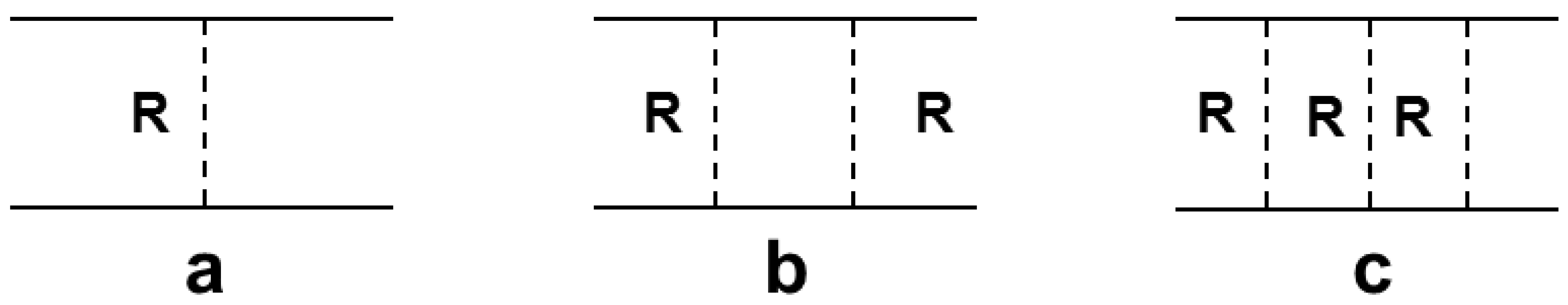
Fig. 90 Nonenhanced diagrams of \(NN\) -scattering.

Taking into account the contributions of other diagrams, shown in Fig. 90, one can find the \(NN\)-scattering amplitude:

\[\gamma_{NN}(\vec b, \xi)=1- e^{-A^{R}_{NN}(\vec{b},\xi)}\]

The calculation of amplitudes and cross sections for cascade interactions requires to consider the so-called enhanced diagrams, like those shown in Fig. 91.

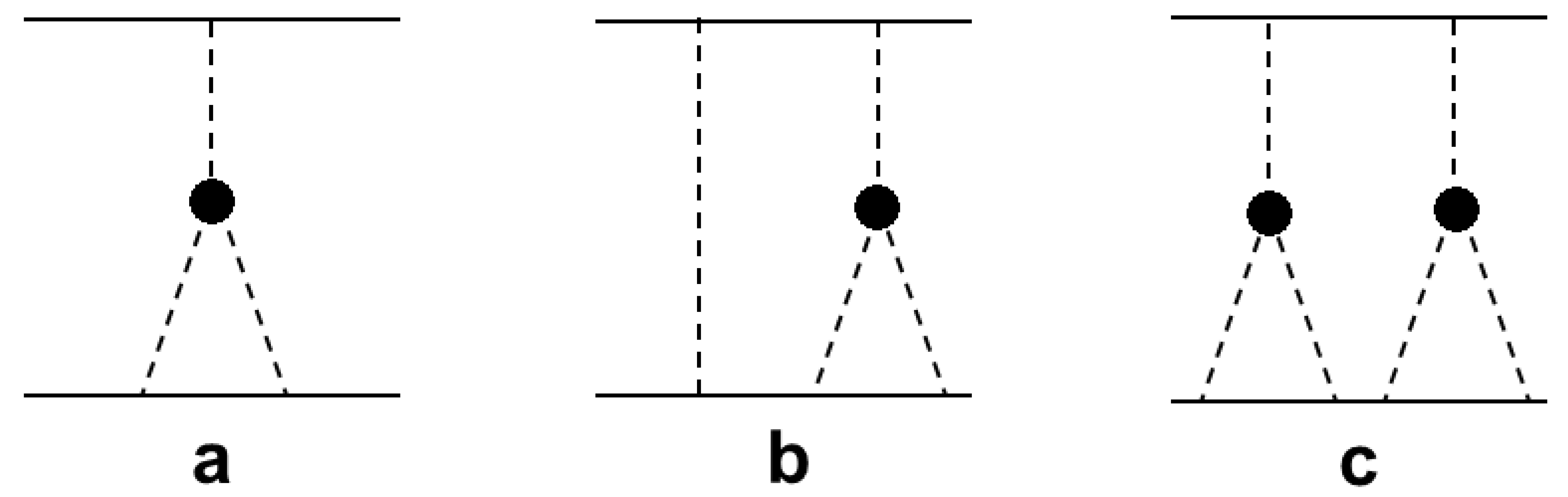
Fig. 91 Simplest enhanced diagrams of \(NN\) -scattering.

The contribution of the diagram in Fig. 91a to the elastic scattering amplitude is given by the expression:

\[G E_{a}(\vec{b},\xi)=-G \int\limits_{\epsilon}^{\xi-\epsilon} d\xi'\int d^{2}b' A^{R_{1}}_{N\pi}(\vec{b}-\vec{b'},\xi-\xi') A^{R_{2}}_{\pi N}(\vec{b'},\xi') A^{R_{3}}_{\pi N}(\vec{b'},\xi')\]

where \(A_{\pi N}\) is the amplitude of meson-nucleon scattering due to one-reggeon exchange, \(G\) is the three reggeon’s coupling constant, \(\epsilon\) is the cutoff parameter (\(\epsilon\sim 1\)). Here we use the model of multi-reggeon vertices proposed in [KpTM86], where it was assumed that reggeons are coupled to one another via a created virtual meson (pion) pair.

The simplest enhanced diagrams for hadron-nucleus scattering were evaluated in [JDTreliani76][Sar80]. An effective computational procedure was proposed in papers [Sch75][CSRJenco76], but it was not applied to the analysis of experimental data. The structure of the enhanced diagrams and their analytical properties were studied in [BKKS91].

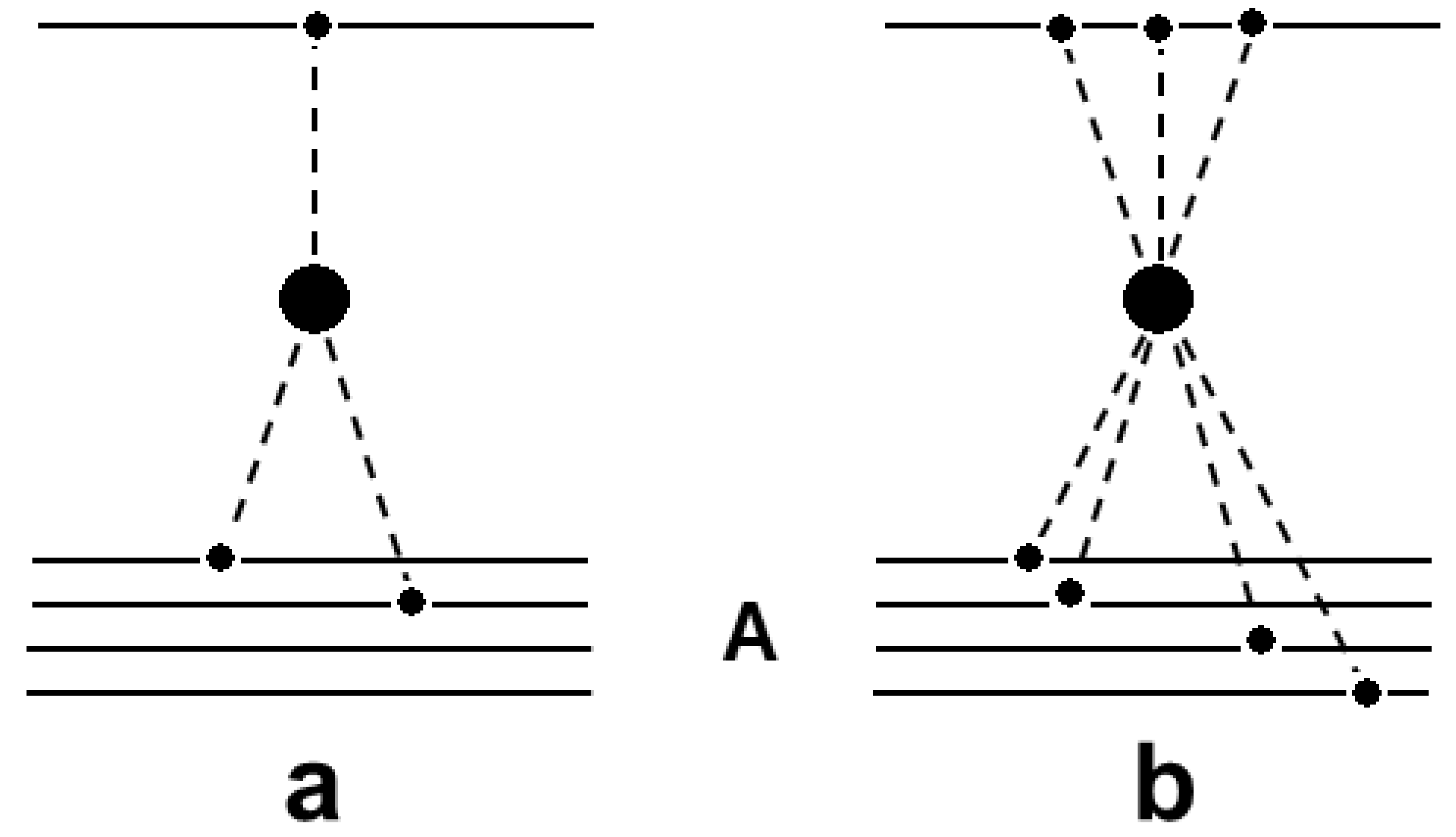
Fig. 92 Possible enhanced diagrams of \(hA\) -interactions.

In the reggeon approach the interaction of secondary particles with a nucleus is described by cuttings of enhanced diagrams. Here the Abramovski-Gribov-Kancheli (AGK) cutting rules [AGK74] are frequently applied. The corrections to them were discussed in [BKKS91] for the problem of particle cascading into the nucleus. It was shown there that inelastic rescatterings occur for any secondary particle, both slow and fast, and the contributions of enhanced diagrams lead to the enrichment of the spectrum by slow particles in the target fragmentation region.

As in [KpTM86] we shall assume that the reggeon interaction vertices are small. Therefore of the full set of enhanced diagrams the only important ones will be those containing vertices where one of the reggeons split into several, which then interact with different nucleons of the nucleus (Fig. 92a). In studying interactions with nuclei, however, it is convenient, in the spirit of the Glauber approach, to deal not with individual reggeons, but with sets of them interacting with a given nucleon of the nucleus (Fig. 92b). Unfortunately, the reggeon method of calculating the sum of the contributions of enhanced diagrams in the case of \(hA\)- and \(AA\)-interactions is not developed for practical tasks. Hence we propose a simple model of estimating reggeon cascading in \(hA\)- and \(AA\)-interactions.

Let us consider the contribution of the first diagram of Fig. 92a:

\[Y= G \int d\xi' d^{2}b' F_{N \pi}(\vec{b} -\vec{b'}, \xi -\xi') \times F_{\pi N}(\vec{b'} -\vec{s}_{1},\xi') F_{\pi N}(\vec{b'} -\vec{s}_{2}, \xi')\]

where \(\vec{b}\) is the impact parameter of a projectile hadron, \(\vec{s}_{1}\) and \(\vec{s}_{2}\) are impact coordinates of two nuclear nucleons, \(\vec {b'}\) is the position of the reggeon interaction vertex in the impact parameter plane, \(\xi'\) is its rapidity.

Using a gaussian parameterization for \(F_{N \pi}\) (\(F_{\pi N}=\exp(-|\vec{b}|^{2}/ R^{2}_{\pi N})\)) and neglecting its dependence on energy, we have

\[Y \simeq G(\xi_{0} -2\epsilon ) \frac{R^{2}_{\pi N}}{3} \exp(-(\vec{b}-(\vec{s}_{1} +\vec{s}_{2})/2)^{2} / 3R^{2}_{\pi N}) \times \exp(-(\vec{s}_{1} -\vec{s}_{2})^{2}/ 2R^{2}_{\pi N})\]

where \(R_{\pi N}\) is the pion-nucleon interaction radius. According to this expression, the contribution reaches a maximum when the nucleon coordinates, \(\vec{s}_{1}\) and \(\vec{s}_{2}\), coincide, and decreases very fast with increasing distance between the nucleons.

Cutting the diagram, one can obtain that the probability, \(\phi\), to involve 2 neighboring nucleons is

\[\phi(\mid \vec{s}_{1} -\vec{s}_{2} \mid)\sim \exp \left(-\frac{\mid \vec{s}_{1} -\vec{s}_{2}\mid^{2}} {R^{2}_{\pi N}} \right)\]

Schematically, the hadron-nucleus interaction process in the impact parameter plane can be represented as in Fig. 93, where the position of the projectile hadron is marked by an open circle, the positions of nuclear nucleons by closed circles, reggeon exchanges by dashed lines and the small points are the coordinates of the reggeon interaction vertices.

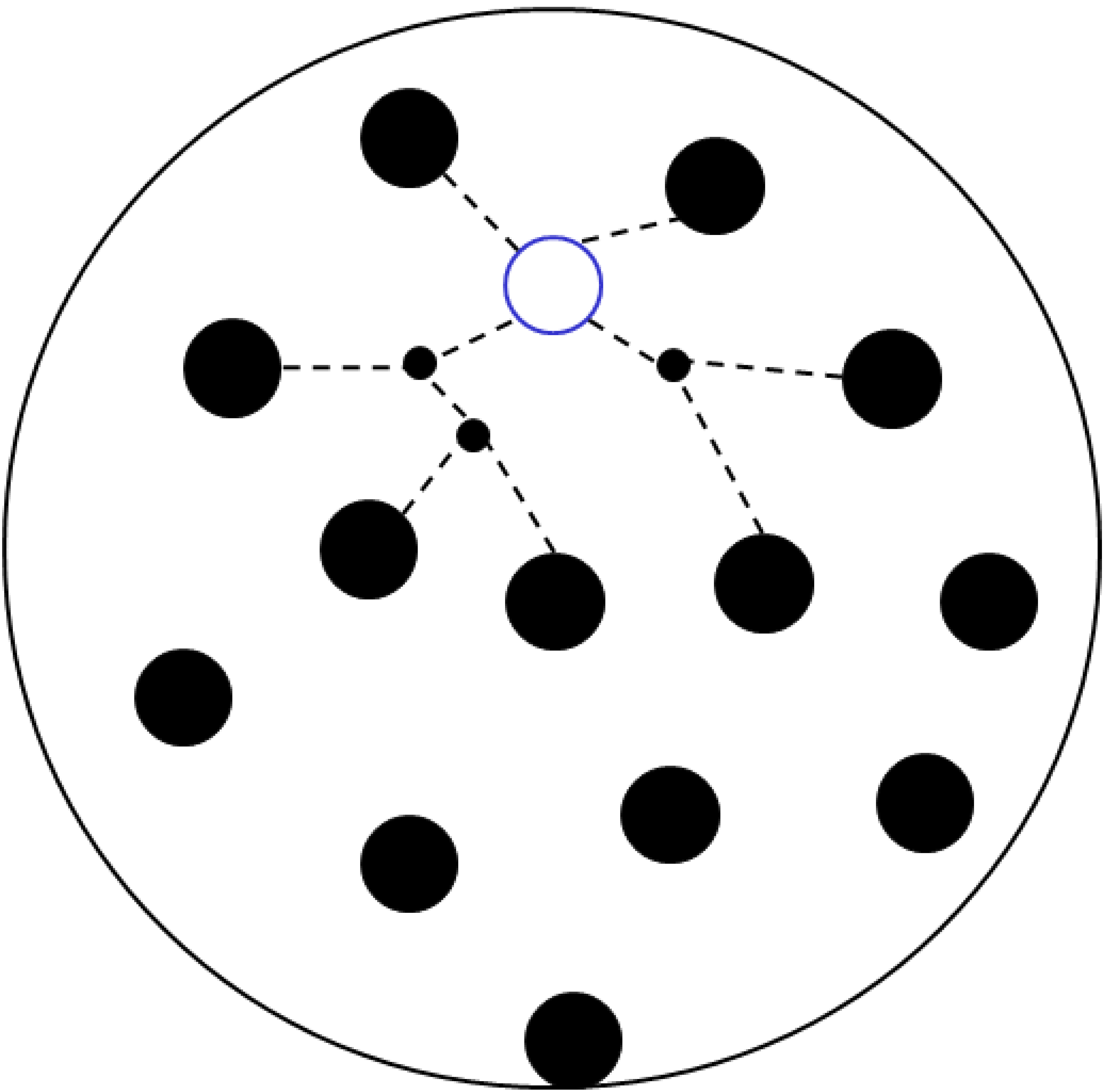
Fig. 93 Reggeon “cascade” in hA-scattering.

Let us consider the problem by using the quark-gluon approach. There were some successful attempts to describe the hadron-nucleon elastic scattering at low and intermediate energies (below 1 – 2 GeV) within this approach (see [BESSwanson92][TBarnesESSwansonJWeinstein92][TBarnesSCapstickMDKovarikS93][TBarnesESSwanson92]). In particular, in the paper [BESSwanson92] the theoretical calculations of the amplitudes of \(\pi\pi\)-, \(KK\)- and \(NN\)-scatterings were found in agreement with experimental data, assuming that in the elastic hadron scattering one-gluon exchange with following quark interchange between hadrons takes place (see Fig. 94a). At high energies, two-gluon exchange approximation (Fig. 94b) works quite well (see [Low75][Nus76][GDShoper77][LR81]). What kind of exchanges can dominate in hadron-nucleus and nucleus-nucleus interactions?

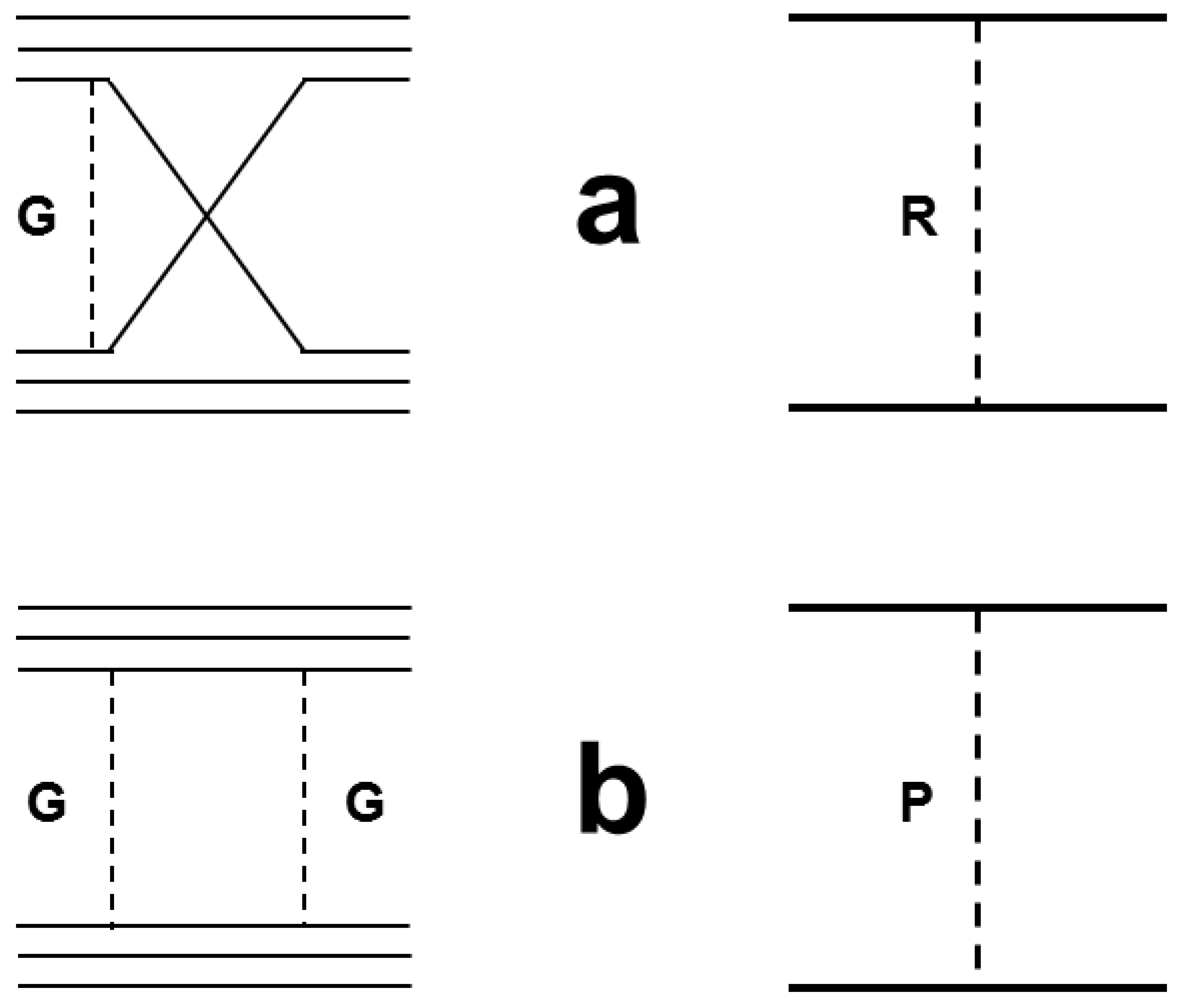
Fig. 94 Diagrams of quark-gluon exchanges and corresponding reggeon diagrams for hadron-nucleus interactions.

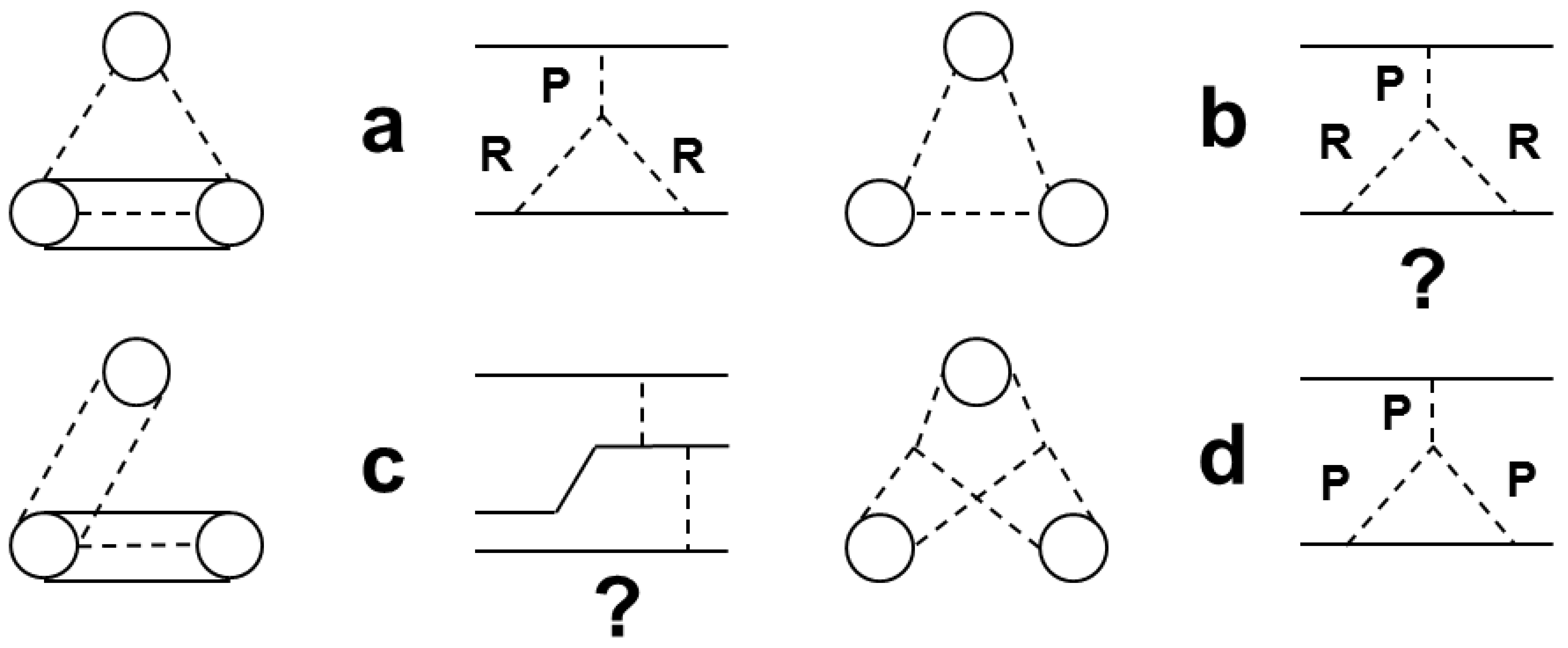
Fig. 95 Diagrams of quark-gluon exchanges and corresponding reggeon diagrams for hadron-nucleus interactions.

The simplest possible diagrams of processes with three nucleons are given in Fig. 95. A calculation of their amplitudes according to [BESSwanson92] is a serious mathematical problem. It can be simplified if one takes into account an analogy between quark-gluon diagrams and reggeon diagrams: the quark diagram of Fig. 94a corresponds to a one-nonvacuum reggeon exchange; the diagram of Fig. 94b describes the pomeron exchange in the \(t\)-channel; the diagram of Fig. 95a is in correspondence with the enhanced reggeon diagram of the pomeron splitting into two non-vacuum reggeons. The three pomeron diagram (Fig. 95d) represents a more complicated process. It is rather difficult to find a correspondence between reggeon diagrams and the diagrams of Fig. 95b, Fig. 95c.

It seems obvious that the processes like one in Fig. 95d cannot dominate in the elastic hadron-nucleus scattering because they are accompanied by a production of high-mass diffractive particles in the intermediate state. Thus, their contributions are damped by a nuclear form-factor. For the same reason, the contributions of processes like the ones in Fig. 95a, Fig. 95b can be small too. If this is not the case, then one can expect large corrections to Glauber cross sections. The practice shows that the corrections to hadron-nucleus cross sections must be lower than 5–7%.

The diagram Fig. 95c can give a correction to the Glauber one-scattering amplitude. Analogous corrections exist for the other terms of Glauber series. They can re-normalize the nuclear vertex constants. According to [BESSwanson92] the contribution has the form:

\[Y_c\propto \exp{[-(\vec b-\vec s_1)/R_p^2]}\exp{[-(\vec s_1-\vec s_2)/R_c^2]}\]

where \(R_p\) is the radius of high-energy nucleon-nucleon interactions, and \(R_c\) is another low-energy radius. Let us note that \(Y_c\) does not depend, as other reggeon diagram contributions, on the longitudinal coordinates of nucleons and the multiplicity of produced particles. This is the main difference between “reggeon cascading” and usual cascading.

As well known, the intra-nuclear cascade models assume that in a hadron-nucleus collision secondary particles are produced in the first inelastic interaction of the projectile with a nuclear nucleon. The produced particles can interact with other target nucleons. The distribution of the distance \(l\) between the first interaction and the second one has the form:

\[W(l)dl\propto \frac{n}{\langle l \rangle} \exp \left(-\frac{n}{\langle l \rangle }\ l\right)\]

where \(\langle l \rangle =1/\sigma\rho_A\), \(\sigma\) is the hadron-nucleon cross section, \(n\) is the multiplicity of the produced particles, and \(\rho_A\sim 0.15\ (\mbox{fm})^{-3}\) is the nuclear density. At the same time, the amplitudes or cross sections of processes like Fig. 95 have no dependence on \(l\) or \(n\). Thus, one can expect that the “cascade” in the quark-gluon approach will be more restricted than in the cascade models. The difference between these approaches can lead to different predictions for hadron interactions with heavy nuclei due to the large multiplicity of the produced particles.

Because it is complicated to calculate the contributions of various diagrams, and to take into account all possibilities, let us formulate a simpler phenomenological model that keeps the main features of the above approaches.

The model formulation

1. As it was said above, the “reggeon” cascade is developed in the impact parameter plane, and has features typical for branching processes. Thus, for its description it is needed to determine the probability to involve a nuclear nucleon into the “cascade”. It is obvious that the probability depends on the difference of the impact coordinates of the new and previous involved nucleons. Looking at the contribution of the diagram Fig. 95c, the functional form of the probability is chosen as:

   (243)\[P(|\vec s_i-\vec s_j|)=C_{nd}\ \exp{[-(\vec s_i-\vec s_j)^2/R_c^2]}\]

   where \(\vec s_i\) and \(\vec s_j\) are the projections of the radii of the i\(^{th}\) and j\(^{th}\) nucleons on the impact parameter plane.

2. The “cascade” is initiated by the primary involved nucleons. These nucleons are determined with the help of the Glauber approach.

3. All involved nucleons are ejected from the nucleus.

The “cascade” looks like that: a projectile particle interacts with some intra-nuclear nucleons. These nucleons are called “wounded” or “participating” nucleons. These nucleons initiate the “cascade”. A wounded nucleon can involve a “spectator” nucleon into the “cascade” with the probability (243). A spectator nucleon can involve another nucleon, which in turn can involve a third one and so on. This algorithm is implemented in the FTF model.

We have tuned \(C_{nd}\) using the HARP-CDP data on proton production in the \(p+Cu\) interactions [eal09]. According to our estimations,

\[C_{nd}= e^{4\ (y-2.1)}/[1 + e^{4\ (y-2.1)}],\ \ \ R_c^2=1.5 \ \ (\mbox{fm})^2\]

where \(y\) is the projectile rapidity. The value of the exponent, \(2.1\), corresponds to \(P_{lab}\sim 4\) GeV/c.

“Fermi motion” of nuclear nucleons

In the “standard” approach, a nucleus is considered as a potential well where nucleons are freely moving. A particle falling on the nucleus changes its momentum on the border of the well. Here a question appears: to whom the recoil momentum must be ascribed? If the particle is absorbed by the nucleus, probably, one has to imagine in the final state the potential well with its nucleons moving with a momentum of the particle. If some nucleons are ejected from the nucleus, what conditions have to satisfy the nucleon momenta, and how will the “residual” well be moving to satisfy the energy-momentum conservation law? In the case of a 3-dimensional potential well, how will be changed the momentum components of a particle on the well surface? Will only the component transverse to the surface, or the one parallel to the surface, or both be changed? The list of questions can be extended by considering nucleus-nucleus interactions.

Two approaches are frequently used in practice.

According to the first one, the nucleus is considered as a continuous medium, and nucleons appeared only in points of the projectile interactions with the medium. It seems natural in this approach to sum the momenta of all ejected particles. Then, subtracting it from the initial momentum, one can find the momentum of the residual nucleus. It is unclear, however, what has to be done in the case of nucleus-nucleus interactions.

In the second approach, space coordinates and momenta of the nucleons are sampled according to some assumptions. In order to satisfy the energy-momentum conservation law, the projectile momentum does not changed, and to each nucleon is ascribed a new mass:

\[m=\sqrt{(m_0-\epsilon_b)^2-p^2}\]

where \(m_0\) is the nucleon mass in the free state, \(\epsilon_b\) is the nuclear binding energy per nucleon, and \(p\) is the momentum of the nucleon. In this approach, the nucleus is a collection of off-mass-shell particles. Apparently, in the case of nucleus-nucleus interactions one has to consider two of such collections. The energy-momentum conservation law is satisfied in this approach if it is satisfied in each collision of out-of-mass-shell nucleons. However, there is a problem with the excitation energy of the nuclear residual: in most of the cases, it is too small.

All these questions are absent in the approach proposed in the paper [eal97].

Let us consider it starting from a simple example of a hadron interaction with a bound system of two nucleons, \((1,2)\). In this approach it is assumed that the process has two stages. At the first one, the system is dissociated:

\[h+(1,2)\rightarrow h+1+2\]

At the second stage a “hard” collision of the projectile with the first or second nucleon takes place. Neglecting transverse momenta let us write the energy-momentum conservation law in the form:

\[\begin{split}\left\{ \begin{array}{l}p_h=p_h'+p_1+p_2\\ E_h+E_{(1,2)}=E_h'+E_1+E_2 \end{array} \right.\end{split}\]

In the above expressions, there are three variables and two equations. Thus, only one variable can be chosen as independent. It can be \(p_h'\) – hadron momentum in the final state, or \(p_1\) or \(p_2\) – nucleon momentum in the final state. We choose as the variable the light-cone momentum fraction of one of the final-state nucleons:

\[x_1=(E_1-p_1)/(E_1+E_2-p_1-p_2)\]

This variable is invariant under the Lorentz transformation along the collision axis.

Using this variable and the energy-momentum conservation law, one can find:

\[W^-=E_1+E_2-p_1-p_2=[s-m_h^2+\beta^2-\lambda^{1/2}(s,m_h^2,\beta^2)]/2\ W_0^+\]

where:

\[\begin{split}W_0^+ & = E_h+E_{(1,2)}+p_h ,\ \ \ W_0^- = E_h+E_{(1,2)}-p_h \\ s & = W_0^+W_0^- ,\ \ \ \ \beta^2 = \frac{m_1^2}{x_1}+\frac{m_2^2}{1-x_1}\end{split}\]

(See (237) for the definition of \(\lambda()\).)

The other kinematical variables are:

\[\begin{split}p_1 & = \frac{m_1^2}{2 x_1 W^-}- \frac{x_1 W^-}{2} ,\ \ \ E_1=\frac{m_1^2}{2 x_1 W^-}+ \frac{x_1 W^-}{2} \\ p_2 & = \frac{m_2^2}{2 (1-x_1) W^-}- \frac{(1-x_1) W^-}{2},\ \ \ E_2=\frac{m_2^2}{2 (1-x_1) W^-}+ \frac{(1-x_1) W^-}{2} \\ p_h' & = p_h-p_1-p_2 ,\ \ \ E_h'=E_h+E_{(1,2)}-E_1-E_2\end{split}\]

So, for the simulation of the interactions, one has to determine only one function: \(f(x_1)\) – the distribution of \(x_1\). Distributions for \(p_1\) and \(p_2\) have interesting properties: at \(p_h \rightarrow \infty\) they become stable (i.e. the distributions remain nearly unchanged when we vary \(p_h\), for large values of \(p_h\)), thus reproducing the typical “limiting fragmentation” (according to an old terminology) of bound system; at \(p_h \rightarrow 0,\ \ \ E_h+E_{(1,2)}>m_h+m_1+m_2\) the distributions \(p_1\) and \(p_2\) become narrower and narrower (i.e. similar to a \(\delta\)-Dirac distribution).

It is not complicated to introduce transverse momenta – \(p_{\perp h}'\), \(p_{\perp 1}\) and \(p_{\perp 2}\), such that \(p_{\perp h}'+p_{\perp 1}+p_{\perp 2}=0\). It is sufficient to replace the masses with the the transverse ones: \(m_i \rightarrow m_{\perp i}=\sqrt{m_i^2+p_{\perp i}^2}\).

In the case of interactions of two composed systems, \(A\) and \(B\), consisting of \(A\) and \(B\) constituents respectively (for brevity, we denote with the same symbol both a composed system and the number of its constituents), let us describe the \(i^{th}\) constituent of \(A\) by the variables:

\[x^+ _i =(E_{Ai} + p_{iz})/W^+ _A ~~~ \text{and} ~~~\vec p _{i\perp}\]

and the \(j^{th}\) constituent of \(B\) by the variables:

\[y^- _j =(E_{Bj} - q_{jz})/W^- _B ~~~ \text{and} ~~~ \vec q _{i\perp}\]

Here \(E_{Ai} (E_{Bi})\) and \(\vec p_i (\vec q_i )\) are energy and momentum of the \(i^{th}\) constituent of the system \(A\) (\(B\)).

\[W^+ _A = \sum ^{A} _{i=1} (E_{Ai} + p_{iz}) ,~~~ W^- _B = \sum ^{B} _{i=1} (E_{Bi} - q_{iz})\]

Using these variables, the energy-momentum conservation law takes the form:

(244)\[\begin{split}\frac{W^+ _A}{2} + \frac {1}{2 W^+ _A} \sum ^{A} _{i=1} \frac {m^2_{i\perp}}{x^+ _i} + \frac{W^- _B}{2} + \frac {1}{2 W^- _B} \sum ^{B} _{i=1} \frac {\mu ^2_{i\perp}}{y^- _i} & = E^0 _A + E^0 _B \\ \frac{W^+ _A}{2} - \frac {1}{2 W^+ _A} \sum ^{A} _{i=1} \frac {m^2_{i\perp}}{x^+ _i} - \frac{W^- _B}{2} + \frac {1}{2 W^- _B} \sum ^{B} _{i=1} \frac {\mu ^2_{i\perp}}{y^- _i} & = P^0 _A + P^0 _B \\ \sum ^{A} _{i=1} \vec p _{i\perp} + \sum ^{B} _{i=1} \vec q _{i\perp} & = 0\end{split}\]

where \(m^2_{i\perp}=m^2_i + \vec p_{i\perp}^2\), \(\mu^2 _{i\perp}=\mu^2_i + \vec q _{i\perp}^2\), and \(m_i (\mu _i )\) is the mass of \(i^{th}\) constituent of the system \(A\) (\(B\)).

The system of equations (244) allows one to find \(W^+ _A,\ \ W^- _B\) and all kinematical properties of the particles at given \(\{x^+ _i , \vec p _{i\perp} \}\), \(\{ y^- _i , \vec q _{i\perp} \}\).

\[\begin{split}W^+ _A & = (W^- _0 W^+ _0 + \alpha - \beta + \sqrt{\Delta})/2W^- _0 \\ W^- _B & = (W^- _0 W^+ _0 - \alpha + \beta + \sqrt{\Delta})/2W^+ _0 \\ W^+ _0 & = (E^0 _A + E^0 _B) + (P^0 _{Az} + P^0 _{Bz}) \\ W^- _0 & = (E^0 _A + E^0 _B) - (P^0 _{Az} + P^0 _{Bz}) \\ \alpha & = \sum ^{A} _{i=1} \frac {m^2 _{i\perp}}{x^+ _i} , ~~~ \beta =\sum ^{B} _{i=1} \frac {\mu ^2 _{i\perp}}{y^- _i} \\ \Delta & = (W^- _0 W^+ _0 )^2 + \alpha ^2 + \beta ^2 - 2 W^- _0 W^+ _0 \alpha - 2 W^- _0 W^+ _0 \beta - 2 \alpha \beta \\ p_{iz} & = (W^+ _A x^+ _i - \frac {m^2 _{i\perp}}{x^+ _i W^+ _A})/2 ;~~~ q_{iz}=-(W^- _B y^- _i - \frac {\mu ^2 _{i\perp}}{y^- _i W^- _B})/2\end{split}\]

Consequently, the problem of accounting for the binding energy and Fermi motion in the simulation of interacting composed systems comes to the definition of the distributions for \(x^+ _i , y^- _i , \vec p _{i\perp}, \vec q _{i\perp}\).

The transverse momentum of an ejected nucleon (\(\vec p _{\perp}\)) is sampled according to the distribution:

\[dW \propto \exp(- \vec p _{\perp} ^2 / \langle p_{\perp} ^2 \rangle ) d^2 p_{\perp}\]

\[\langle p_{\perp} ^2 \rangle =0.035+0.04\frac{e^{4\ (y_{lab}-2.5)}}{1+e^{4\ (y_{lab}-2.5)}}\ \ \ (\mbox{GeV}/c)^2\]

where \(y_{lab}\) is the projectile nucleus rapidity in the rest frame of the target nucleus. The sum of the transverse momenta with minus sign is ascribed to the residual of the target nucleus.

\(x^+\) (and similarly for \(y^-\)) is sampled according to the distribution:

\[dW \propto \exp[- (x^+ -1/A)^2/(d /A)^2 ] d x^+ ,~~~d =0.3\]

\(x^+\) of the nuclear residual is determined as \(1 - \sum x^+ _i \).

Excitation energy of nuclear residuals

According to the approach presented above, the excitation energy of a nuclear residual has to be determined before the simulation of particle production. It seems natural to assume that this excitation energy is connected with the multiplicity of ejected nuclear nucleons, both the participating ones and those involved in the reggeon cascading. Without the involved nucleons, the excitation energy would be proportional to the multiplicity of the participating nucleons as calculated in the Glauber approach. Such approach was followed in the paper [AMWAFriedmanJHufner86], where proton-nucleus interactions at intermediate energies were analyzed. There the multiplicity of the nucleons was calculated in the Glauber approach. It was also assumed that each recoil of the participating nucleons contributes to the excitation energy with a value sampled from the following distribution:

\[dW(E)=\frac{1}{\langle E \rangle}e^{-E/\langle E \rangle}dE\]

The sum of these contributions determines the residual excitation energy. The authors of the paper [AMWAFriedmanJHufner86] considered both absorptions and ejections of the nucleons, and took into account the effect of decreasing projectile energy during the interactions. They obtained a good agreement of their calculations with experimental data on neutron production as a function of the residual excitation energy.

Extending this approach, we assume, as a first step, that each participating or involved nucleon adds 100 MeV to the nuclear residual excitation energy. The excited residual is then fragmented by using the Generalized Evaporation Model (GEM) [Fur00].

Bibliography

AWU97

K. Abdel-Waged and V. V. Uzhinsky. Model of nuclear disintegration in high-energy nucleus nucleus interactions. Phys. Atom. Nucl., 60:828–840, 1997. [Yad. Fiz.60,925(1997)].

AWU98

Kh Abdel-Waged and V V Uzhinskii. Estimation of nuclear destruction using ALADIN experimental data. Journal of Physics G: Nuclear and Particle Physics, 24(9):1723–1733, sep 1998. URL: https://doi.org/10.1088/0954-3899/24/9/006, doi:10.1088/0954-3899/24/9/006.

AGK74(1,2)

V.A. Abramovsky, V.N. Gribov, and O.V. Kancheli. Sov. J. Nucl. Phys., 18:308, 1974. Russian original: Yad. Fiz. \bf 18 595 (1973).

AMWAFriedmanJHufner86(1,2)

A.Y. Abul-Magd, W.A.Friedman, and J.Hufner. Phys. Rev. C, 34():113, 1986.

ABLaPS05

B. Alver, M. Baker, C. Loizides, and and P. Steinberg. pre-print, 2005. arxiv:0805.4411 [nucl-exp].

BNilssonAEStenlund87

B.Nilsson-Almquist and E.Stenlund. Comp. Phys. Comm., 43:43, 1987.

BESSwanson92(1,2,3,4)

T. Barnes and E.S.Swanson. Phys. Rev. D, 46:131, 1992.

BKKS91(1,2)

K.G. Boreskov, A.B. Kaidalov, S.M. Kiselev, and N.Ya. Smorodinskaya. Sov. J. Nucl. Phys., 53():356, 1991. Russian original: Yad. Fiz. \bf 53 569 (1991).

BRaPB09

W. Broniowski, M. Rybczynski, and and P. Bozek. Comp. Phys. Commun., 180:69, 2009.

CSRJenco76

L. Caneschi, A. Schwimmer, and R.Jenco. Nucl. Phys. B, 108:82, 1976.

eal87

B.Andersson et al. Nucl. Phys. B, 281:289, 1987.

eal72(1,2)

E. Bracci et al. Technical Report CERN–HERA 72-1, CERN, 1972.

eal73a(1,2)

E. Bracci et al. Technical Report 73-1, CERN–HERA, 1973.

eal99

M. Bleicher et al. J. Phys. G, 25:1859, 1999.

eal73b

P. Bosettii et al. Nucl. Phys. B, 54:141, 1973.

eal98

S.A. Bass et al. Prog. Part. Nucl. Phys., 41:225, 1998.

eal84(1,2)

V. Flaminio et al. Technical Report 84-01, CERN–HERA, 1984.

ealCOMPLETEcollab02

J.R. Cudell et al. (COMPLETE collab.). Phys. Rev. D, 65:074024, 2002.

eal77

BBCMS Collab. (I.V. Azhinenko et al.). Nucl. Phys. B, 123:493, 1977.

eal74

Bonn-Hamburg-Munich Collab. (V. Blobel et al.). Nucl. Phys. B, 69:454, 1974.

eal97

EMU-01 Collab. (M.I. Adamovich et al.). Zeit. fur Phys. A, 358:337, 1997.

eal09

HARP-CDP Collab. (A. Bolshakova et al.). Eur. Phys. J. C, 64:181, 2009.

eal86

NA22 Collab. (M. Adamus et al.). Zeit. fur Phys. C, 32:475, 1986.

FIW04

G. Folger, V. N. Ivanchenko, and J. P. Wellisch. The binary cascade. The European Physical Journal A, 21(3):407–417, sep 2004. URL: https://doi.org/10.1140/epja/i2003-10219-7, doi:10.1140/epja/i2003-10219-7.

Fra68

V. Franco. Phys. Rev., 175:1376, 1968.

Fur00

S. Furihata. Nuclear Instruments and Methods in Physics Research B, 171():251, 2000.

Gla59

R.J. Glauber. “Lectures in Theoretical Physics”, Ed. W.E.Brittin et al. Interscience Publishers, N.Y., vol. 1 edition, 1959.

Gla67

R.J. Glauber. In Ed. G.A.Alexander, editor, Proc. of the 2nd Int. Conf. on High Energy Physics and Nuclear structure. Rehovoth, 1967. North-Holland, Amsterdam.

GM99(1,2)

K.A. Goulianos and J. Montanha. Phys. Rev. D, 59:114017, 1999.

GDShoper77

J. Gunion and D.Shoper. Phys. Rev. D, 15():2617, 1977.

JDTreliani76

R. Jengo and D.Treliani. Nucl. Phys. B, 117:433, 1976.

KpTM86(1,2)

A.B. Kaidalov, L.A. ponomarev, and K.A. Ter-Martirosian. Sov. J. Nucl. Phys., 44:468, 1986. Russian original: Yad. Fiz. \bf 44 722 (1986).

KV94

A.B. Kaidalov and P.E. Volkovitsky. Zeit. fur Phys., C63:517, 1994.

LR81

E.M. Levin and M.G. Ryskin. Yad. Fiz., 34:619, 1981.

Low75

F. Low. Phys. Rev. D, 12:163, 1975.

MRSS07

M.L. Miller, K. Reygers, S.J. Sanders, and P. Steinberg. Ann. Rev. Nucl. Part. Sci., 57:205, 2007.

Nus76

S. Nussinov. Phys. Rev. D, 14():246, 1976.

PDG12(1,2,3,4)

PDG. Pdg 2012 online reference. http://pdg.lbl.gov/2012/hadronic-xsections/hadron.html, 2012. [Online; accessed 26-october-2017].

Sar80

R.E. Camboa Saravi. Phys. Rev., 21:2021, 1980.

Sch75

A. Schwimmer. Nucl. Phys. B, 94:445, 1975.

Sha81

Yu.M. Shabelski. Sov. J. Part. Nucl., 12:430, 1981.

SUZ89

S.Yu. Shmakov, V.V. Uzhinski, and A.M. Zadorojny. Comp. Phys. Commun., 54:125, 1989.

TBarnesESSwanson92

T.Barnes and E.S.Swanson. Phys. Rev. C, 49:1166, 1992.

TBarnesESSwansonJWeinstein92

T.Barnes, E.S.Swanson, and J.Weinstein. Phys. Rev. D, 46:4868, 1992.

TBarnesSCapstickMDKovarikS93

T.Barnes, S.Capstick, M.D.Kovarik, and E.S. Swanson. Phys. Rev. C, 48:539, 1993.

UG02

V.V. Uzhinsky and A.S. Galoyan. pre-print, 2002.

Whi74(1,2)

J. Whitmore. Phys. Rep., 10:273, 1974.