Cross-sections in Photonuclear and Electronuclear Reactions

Approximation of Photonuclear Cross Sections

The photonuclear cross sections parameterized in the G4PhotoNuclearCrossSection class cover all incident photon energies from the hadron production threshold upward. The parameterization is subdivided into five energy regions, each corresponding to the physical process that dominates it.

The Giant Dipole Resonance (GDR) region, depending on the nucleus, extends from 10 MeV up to 30 MeV. It usually consists of one large peak, though for some nuclei several peaks appear.
The “quasi-deuteron” region extends from around 30 MeV up to the pion threshold and is characterized by small cross sections and a broad, low peak.
The $\Delta$ region is characterized by the dominant peak in the cross section which extends from the pion threshold to 450 MeV.
The Roper resonance region extends from roughly 450 MeV to 1.2 GeV. The cross section in this region is not strictly identified with the real Roper resonance because other processes also occur in this region.
The Reggeon-Pomeron region extends upward from 1.2 GeV.

In the Geant4 photonuclear data base there are about 50 nuclei for which the photonuclear absorption cross sections have been measured in the above energy ranges. For low energies this number could be enlarged, because for heavy nuclei the neutron photoproduction cross section is close to the total photo-absorption cross section. Currently, however, 14 nuclei are used in the parameterization: ¹H, ²H, ⁴He, ⁶Li, ⁷Li, ⁹Be, ¹²C, ¹⁶O, ²⁷Al, ⁴⁰Ca, Cu, Sn, Pb, and U. The resulting cross section is a function of $A$ and $e = \log(E_\gamma)$, where $E_\gamma$ is the energy of the incident photon. This function is the sum of the components which parameterize each energy region. The cross section in the GDR region can be described as the sum of two peaks,

\[GDR(e) = th(e,b_1,s_1)\cdot \exp(c_1-p_1\cdot e) + th(e,b_2,s_2)\cdot \exp(c_2-p_2\cdot e) .\]

The exponential parameterizes the falling edge of the resonance which behaves like a power law in $E_\gamma$. This behavior is expected from the CHIPS modelling approach ([DKW00]), which includes the nonrelativistic phase space of nucleons to explain evaporation. The function

\[th(e,b,s) = \frac{1}{1+\exp \left(\frac{b-e}{s} \right)} ,\]

describes the rising edge of the resonance. It is the nuclear-barrier-reflection function and behaves like a threshold, cutting off the exponential. The exponential powers $p_1$ and $p_2$ are

\[\begin{split}p_1 = 1, p_2 = 2 & \mbox{ for } A < 4 \\ p_1 = 2, p_2 = 4 & \mbox{ for } 4 \le A < 8 \\ p_1 = 3, p_2 = 6 & \mbox{ for } 8 \le A < 12 \\ p_1 = 4, p_2 = 8 & \mbox{ for } A \ge 12 .\end{split}\]

The $A$-dependent parameters $b_i$, $c_i$ and $s_i$ were found for each of the 14 nuclei listed above and interpolated for other nuclei. The $\Delta$ isobar region was parameterized as

\[\Delta (e,d,f,g,r,q)=\frac{d\cdot th(e,f,g)}{1+r\cdot (e-q)^2},\]

where $d$ is an overall normalization factor. $q$ can be interpreted as the energy of the $\Delta$ isobar and $r$ can be interpreted as the inverse of the $\Delta$ width. Once again $th$ is the threshold function. The $A$-dependence of these parameters is as follows:

$d=0.41\cdot A$ (for ¹H it is 0.55, for ²H it is 0.88), which means that the $\Delta$ yield is proportional to $A$;
$f=5.13-.00075\cdot A$. $\exp(f)$ shows how the pion threshold depends on $A$. It is clear that the threshold becomes 140 MeV only for uranium; for lighter nuclei it is higher.
$g = 0.09$ for $A \ge 7$ and 0.04 for $A < 7$;
$q=5.84-\frac{.09}{1+.003\cdot A^2}$, which means that the “mass” of the $\Delta$ isobar moves to lower energies;
$r=11.9 - 1.24\cdot \log(A)$. $r$ is 18.0 for ¹H. The inverse width becomes smaller with $A$, hence the width increases.

The $A$-dependence of the $f$, $q$ and $r$ parameters is due to the $\Delta+N\rightarrow N+N$ reaction, which can take place in the nuclear medium below the pion threshold. The quasi-deuteron contribution was parameterized with the same form as the $\Delta$ contribution but without the threshold function:

\[QD(e,v,w,u)=\frac {v}{1+w\cdot (e-u)^2}.\]

For ¹H and ²H the quasi-deuteron contribution is almost zero. For these nuclei the third baryonic resonance was used instead, so the parameters for these two nuclei are quite different, but trivial. The parameter values are given below.

$v = \frac {\exp(-1.7+a\cdot 0.84)}{1+\exp(7\cdot (2.38-a))}$, where $a=\log(A)$. This shows that the $A$-dependence in the quasi-deuteron region is stronger than $A^{0.84}$. It is clear from the denominator that this contribution is very small for light nuclei (up to ⁶Li or ⁷Li). For ¹H it is 0.078 and for ²H it is 0.08, so the delta contribution does not appear to be growing. Its relative contribution disappears with $A$.
$u = 3.7$ and $w = 0.4$. The experimental information is not sufficient to determine an $A$-dependence for these parameters. For both $^1$H and $^2$H $u = 6.93$ and $w = 90$, which may indicate contributions from the $\Delta$(1600) and $\Delta$(1620).

The transition Roper contribution was parameterized using the same form as the quasi-deuteron contribution:

\[Tr(e,v,w,u)=\frac {v}{1+w\cdot (e-u)^2}.\]

Using $a=\log(A)$, the values of the parameters are

$v = \exp(-2.+a\cdot 0.84)$. For $^1$H it is 0.22 and for $^2$H it is 0.34.
$u = 6.46+a\cdot 0.061$ (for $^1$H and for $^2$H it is 6.57), so the “mass” of the Roper moves higher with $A$.
$w = 0.1+a\cdot 1.65$. For ¹ H it is 20.0 and for ²H it is 15.0).

The Regge-Pomeron contribution was parametrized as follows:

(283)\[RP(e,h)=h\cdot th(7.,0.2)\cdot (0.0116\cdot \exp(e\cdot 0.16)+0.4\cdot \exp(-e\cdot 0.2)),\]

where $h=A\cdot \exp(-a\cdot (0.885+0.0048\cdot a))$ and, again, $a = \log(A)$. The first exponential in Eq. (283) describes the Pomeron contribution while the second describes the Regge contribution.

Electronuclear Cross Sections and Reactions

Electronuclear reactions are so closely connected with photonuclear reactions that they are sometimes called “photonuclear” because the one-photon exchange mechanism dominates in electronuclear reactions. In this sense electrons can be replaced by a flux of equivalent photons. This is not completely true, because at high energies the Vector Dominance Model (VDM) or diffractive mechanisms are possible, but these types of reactions are beyond the scope of this discussion.

Common Notation for Different Approaches to Electronuclear Reactions

The Equivalent Photon Approximation (EPA) was proposed by E. Fermi [Fer24] and developed by C. Weizsacker and E. Williams [Weizsacker34][Wil34] and by L. Landau and E. Lifshitz [LL34]. The covariant form of the EPA method was developed in Refs. [PS61] and [GSKO62]. When using this method it is necessary to take into account that real photons are always transversely polarized while virtual photons may be longitudinally polarized. In general the differential cross section of the electronuclear interaction can be written as

\[\frac{d^2\sigma}{dydQ^2}=\frac{\alpha}{\pi Q^2}(S_{TL}\cdot(\sigma_T +\sigma_L)-S_L\cdot\sigma_L),\]

where

\[\begin{split}S_{TL} &= y\frac{1-y+\frac{y^2}{2} + \frac{Q^2}{4E^2} -\frac{m^2_e}{Q^2} \left( y^2+\frac{Q^2}{E^2} \right) }{y^2+\frac{Q^2}{E^2}}, \\ S_L & =\frac{y}{2} \left( 1-\frac{2m_e^2}{Q^2} \right) .\end{split}\]

The differential cross section of the electronuclear scattering can be rewritten as

\[\frac{d^2\sigma_{eA}}{dydQ^2}=\frac{\alpha y}{\pi Q^2}\left(\frac{(1-\frac{y}{2})^2} {y^2+\frac{Q^2}{E^2}}+\frac{1}{4}-\frac{m^2_e}{Q^2}\right)\sigma_{\gamma^*A},\]

where $\sigma_{\gamma^*A}=\sigma_{\gamma A}(\nu)$ for small $Q^2$ and must be approximated as a function of $\epsilon$, $\nu$, and $Q^2$ for large $Q^2$. Interactions of longitudinal photons are included in the effective $\sigma_{\gamma^*A}$ cross section through the $\epsilon$ factor, but in the present Geant4 method, the cross section of virtual photons is considered to be $\epsilon$-independent. The electronuclear problem, with respect to the interaction of virtual photons with nuclei, can thus be split in two. At small $Q^2$ it is possible to use the $\sigma_\gamma(\nu)$ cross section. In the $Q^2 \gg m^2_e$ region it is necessary to calculate the effective $\sigma_{\gamma^*}(\epsilon,\nu,Q^2)$ cross section. Following the EPA notation, the differential cross section of electronuclear scattering can be related to the number of equivalent photons $dn=d\sigma/\sigma_{\gamma^*}$. For $y \ ll 1$ and $Q^2<4m^2_e$ the canonical method [VBB71] leads to the simple result

(284)\[\frac{ydn(y)}{dy}=-\frac{2\alpha}{\pi} \ln(y).\]

In [BGMS75] the integration over $Q^2$ for $\nu^2 \gg Q^2_{max}\simeq m^2_e$ leads to

\[\frac{ydn(y)}{dy} = -\frac{\alpha}{\pi} \left[ \frac{1+(1-y)^2}{2} \ln \left( \frac{y^2}{1-y} \right) +(1-y)\right].\]

In the $y \ll 1$ limit this formula converges to Eq. (284). But the correspondence with Eq. (284) can be made more explicit if the exact integral

(285)\[\frac{ydn(y)}{dy}=\frac{\alpha}{\pi}\left( \frac{1+(1-y)^2}{2}l_1-(1-y)l_2-\frac{(2-y)^2}{4}l_3\right),\]

where

\[\begin{split}l_1 &= \ln \left( \frac{Q^2_{max}}{Q^2_{min}} \right), \\ l_2 &= 1 - \frac{Q^2_{max}}{Q^2_{min}}, \\ l_3 &= \ln \left( \frac{y^2+Q^2_{max}/E^2}{y^2+Q^2_{min}/E^2} \right), \\ Q^2_{min} &= \frac{m_e^2y^2}{1-y},\end{split}\]

is calculated for

(286)\[Q^2_{max(m_e)}=\frac{4m^2_e}{1-y}.\]

The factor $(1-y)$ is used arbitrarily to keep $Q^2_{max(m_e)}>Q^2_{min}$, which can be considered as a boundary between the low and high $Q^2$ regions. The full transverse photon flux can be calculated as an integral of Eq. (285) with the maximum possible upper limit

(287)\[Q^2_{max(max)}=4E^2(1-y).\]

The full transverse photon flux can be approximated by

(288)\[\frac{ydn(y)}{dy}=-\frac{2\alpha}{\pi}\left( \frac{(2-y)^2+y^2}{2}\ln(\gamma)-1\right),\]

where $\gamma=E/m_e$. It must be pointed out that neither this approximation nor Eq. (285) works at $y\simeq 1$; at this point $Q^2_{max(max)}$ becomes smaller than $Q^2_{min}$. The formal limit of the method is $y<1-\frac{1}{2\gamma}$.

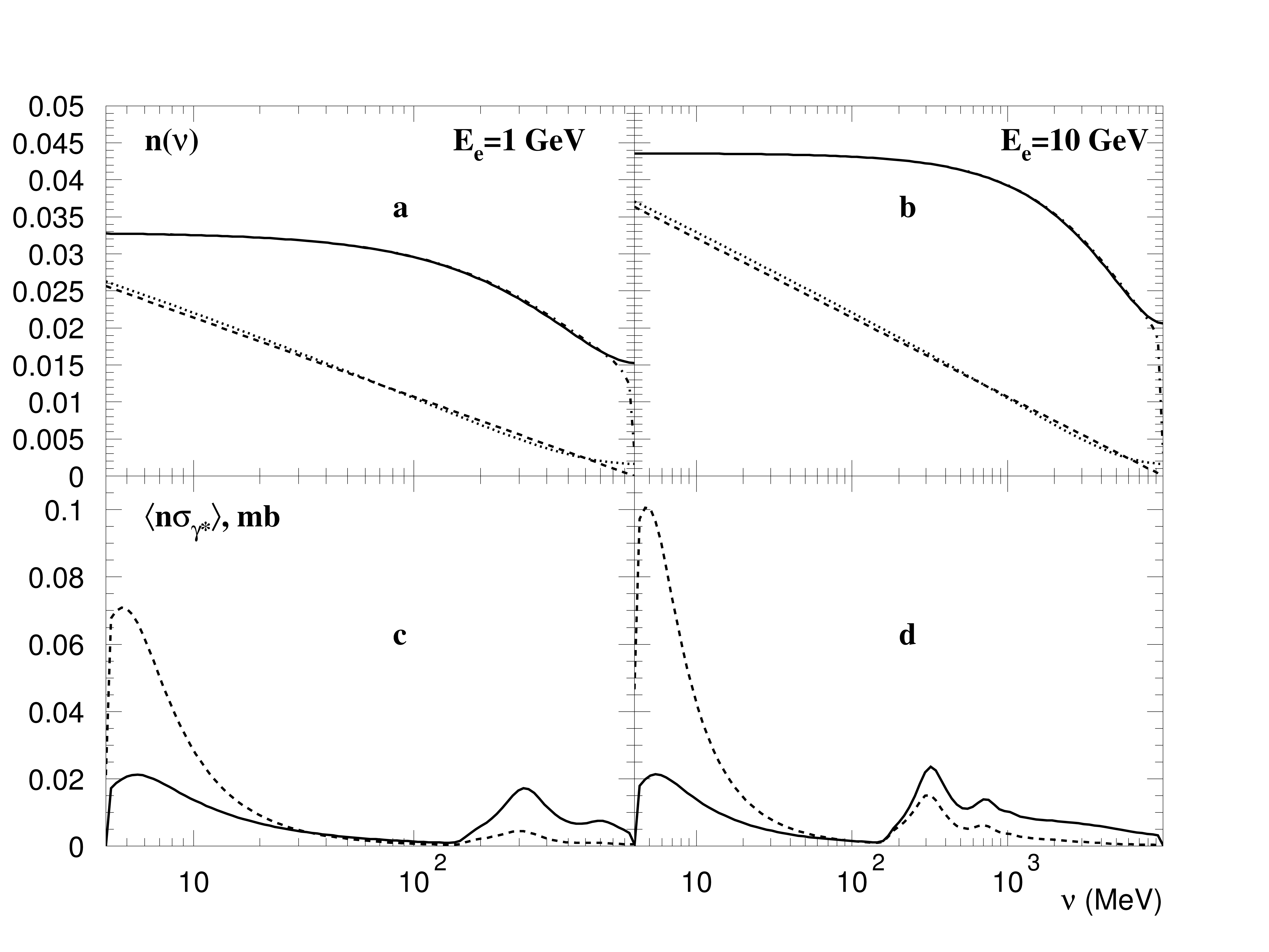
Fig. 120 Relative contribution of equivalent photons with small $Q^2$ to the total “photon flux” for (a) 1 GeV electrons and (b) 10 GeV electrons. In figures (c) and (d) the equivalent photon distribution $dn(\nu,Q^2)$ is multiplied by the photonuclear cross section $\sigma_{\gamma^*}(K,Q^2)$ and integrated over $Q^2$ in two regions: the dashed lines are integrals over the low-$Q^2$ equivalent photons (under the dashed line in the first two figures), and the solid lines are integrals over the high-$Q^2$ equivalent photons (above the dashed lines in the first two figures).

In Fig. 120(a,b) the energy distribution for the equivalent photons is shown. The low-$Q^2$ photon flux with the upper limit defined by Eq. (286) is compared with the full photon flux. The low-$Q^2$ photon flux is calculated using Eq. (284) (dashed lines) and using Eq. (285) (dotted lines). The full photon flux is calculated using Eq. (288) (the solid lines) and using Eq. (285) with the upper limit defined by Eq.(287) (dash-dotted lines, which differ from the solid lines only at $\nu\approx E_e$). The conclusion is that in order to calculate either the number of low-$Q^2$ equivalent photons or the total number of equivalent photons one can use the simple approximations given by Eq. (284) and Eq.(288), respectively, instead of using Eq. (285), which cannot be integrated over $y$ analytically. Comparing the low-$Q^2$ photon flux and the total photon flux it is possible to show that the low-$Q^2$ photon flux is about half of the the total. From the interaction point of view the decrease of $\sigma_{\gamma*}$ with increasing $Q^2$ must be taken into account. The cross section reduction for the virtual photons with large $Q^2$ is governed by two factors. First, the cross section drops with $Q^2$ as the squared dipole nucleonic form-factor

\[G^2_D(Q^2)\approx\left( 1+\frac{Q^2}{(843 \mbox{ MeV})^2}\right)^{-2}.\]

Second, all the thresholds of the $\gamma A$ reactions are shifted to higher $\nu$ by a factor $Q^2/2M$, which is the difference between the $K$ and $\nu$ values. Following the method proposed in [BFG+76] the $\sigma_{\gamma^*}$ at large $Q^2$ can be approximated as

(289)\[\sigma_{\gamma*}=(1-x)\sigma_\gamma(K)G^2_D(Q^2)e^{b(\epsilon,K)\cdot r+c(\epsilon,K)\cdot r^3},\]

where $r=\frac{1}{2}\ln(\frac{Q^2+\nu^2}{K^2})$. The $\epsilon$-dependence of the $a(\epsilon,K)$ and $b(\epsilon,K)$ functions is weak, so for simplicity the $b(K)$ and $c(K)$ functions are averaged over $\epsilon$. They can be approximated as

\[b(K)\approx\left(\frac{K}{185 \mbox{ MeV}}\right)^{0.85},\]

and

\[c(K)\approx-\left(\frac{K}{1390 \mbox{ MeV}}\right)^{3}.\]

The result of the integration of the photon flux multiplied by the cross section approximated by Eq. (289) is shown in Fig. 120(c,d). The integrated cross sections are shown separately for the low-$Q^2$ region ($Q^2, dashed lines) and for the high-\(Q^2$ region ($Q^2>Q^2_{max(m_e)}$, solid lines). These functions must be integrated over $\ln(\nu)$, so it is clear that because of the Giant Dipole Resonance contribution, the low-$Q^2$ part covers more than half the total $eA\rightarrow \mbox{hadrons}$ cross section. But at $\nu$ >200 MeV, where the hadron multiplicity increases, the large $Q^2$ part dominates. In this sense, for a better simulation of the production of hadrons by electrons, it is necessary to simulate the high-$Q^2$ part as well as the low-$Q^2$ part.

Taking into account the contribution of high-$Q^2$ photons it is possible to use Eq. (288) with the over-estimated $\sigma_{\gamma^*A}=\sigma_{\gamma A}(\nu)$ cross section. The slightly over-estimated electronuclear cross section is

\[\sigma^*_{eA}=(2\ln(\gamma)-1)\cdot J_1-\frac{\ln(\gamma)}{E_e} \left( 2J_2-\frac{J_3}{E_e} \right).\]

where

\[\begin{split}J_1(E_e) &= \frac{\alpha}{\pi}\int^{E_e}\sigma_{\gamma A}(\nu)d \ln(\nu) \\ J_2(E_e) &= \frac{\alpha}{\pi}\int^{E_e}\nu\sigma_{\gamma A}(\nu)d \ln(\nu),\end{split}\]

and

\[J_3(E_e)=\frac{\alpha}{\pi}\int^{E_e}\nu^2\sigma_{\gamma A}(\nu) d \ln(\nu).\]

The equivalent photon energy $\nu=yE$ can be obtained for a particular random number $R$ from the equation

\[R=\frac{(2 \ln(\gamma)-1)J_1(\nu)-\frac{\ln(\gamma)}{E_e} \left(2J_2(\nu)-\frac{J_3(\nu)}{E_e}\right) } {(2\ln(\gamma)-1)J_1(E_e)-\frac{\ln(\gamma)}{E_e} \left(2J_2(E_e)-\frac{J_3(E_e)}{E_e} \right)}.\]

Eq. (285) is too complicated for the randomization of $Q^2$ but there is an easily randomized formula which approximates Eq. (285) above the hadronic threshold ($E$ > 10 MeV). It reads

(290)\[\frac{\pi}{\alpha D(y)}\int^{Q^2}_{Q^2_{min}}\frac{ydn(y,Q^2)}{dydQ^2}dQ^2=-L(y,Q^2)-U(y),\]

where

\[\begin{split}D(y) &= 1-y+\frac{y^2}{2}, \\ L(y,Q^2) &= \ln\left[ F(y)+ \left(e^{P(y)}-1+\frac{Q^2}{Q^2_{min}} \right)^{-1} \right],\end{split}\]

and

\[U(y)=P(y)\cdot\left( 1-\frac{Q^2_{min}}{Q^2_{max}}\right),\]

with

\[F(y)=\frac{(2-y)(2-2y)}{y^2}\cdot\frac{Q^2_{min}}{Q^2_{max}}\]

and

\[P(y)=\frac{1-y}{D(y)}.\]

The $Q^2$ value can then be calculated as

\[\frac{Q^2}{Q^2_{min}}=1-e^{P(y)}+\left(e^{R\cdot L(y,Q^2_{max})-(1-R)\cdot U(y)}-F(y) \right)^{-1},\]

where $R$ is a random number. In Fig. 121, Eq. (285) (solid curve) is compared to Eq. (290) (dashed curve). Because the two curves are almost indistinguishable in the figure, this can be used as an illustration of the $Q^2$ spectrum of virtual photons, which is the derivative of these curves. An alternative approach is to use Eq. (285) for the randomization with a three dimensional table $\frac{ydn}{dy}(Q^2,y,E_e)$.

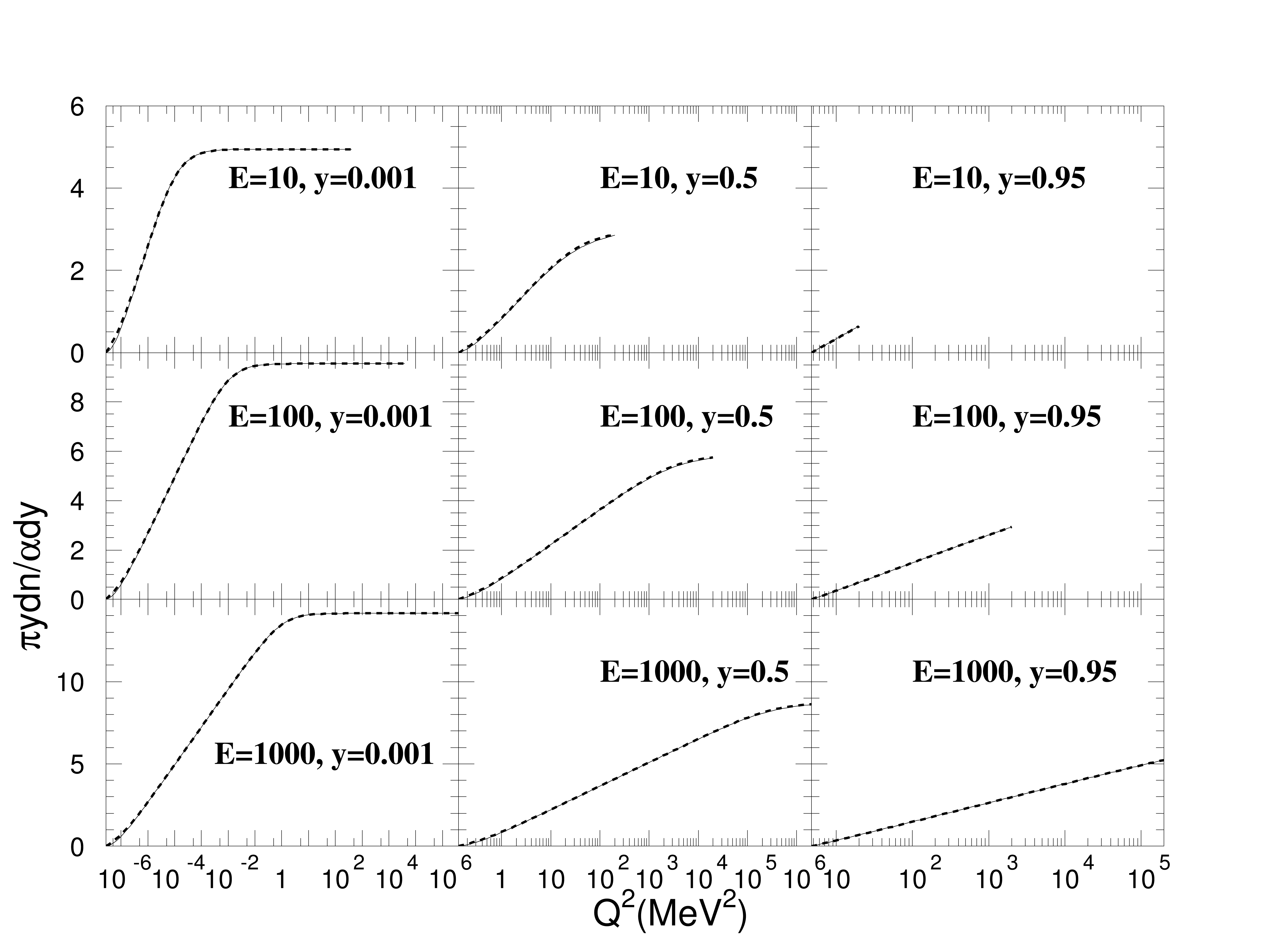
Fig. 121 Integrals of $Q^2$ spectra of virtual photons for three energies 10 MeV, 100 MeV, and 1 GeV at y=0.001, y=0.5, and y=0.95. The solid line corresponds to Eq. (285) and the dashed line (which almost everywhere coincides with the solid line) corresponds to Eq. (285).

After the $\nu$ and $Q^2$ values have been found, the value of $\sigma_{\gamma^*A}(\nu,Q^2)$ is calculated using Eq. (289). If $R\cdot\sigma_{\gamma A}(\nu)>\sigma_{\gamma^*A}(\nu,Q^2)$, no interaction occurs and the electron keeps going. This “do nothing” process has low probability and cannot shadow other processes.

Bibliography

BFG+76: F.W. Brasse, W. Flauger, J. Gayler, S.P. Goel, R. Haidan, M. Merkwitz, and H. Wriedt. Parametrization of the q2 dependence of $\upgamma _v$ p total cross sections in the resonance region. Nuclear Physics B, 110(4-5):413–433, aug 1976. URL: https://doi.org/10.1016/0550-3213(76)90231-5, doi:10.1016/0550-3213(76)90231-5.
BGMS75: V.M. Budnev, I.F. Ginzburg, G.V. Meledin, and V.G. Serbo. The two-photon particle production mechanism. physical problems. applications. equivalent photon approximation. Physics Reports, 15(4):181–282, jan 1975. URL: https://doi.org/10.1016/0370-1573(75)90009-5, doi:10.1016/0370-1573(75)90009-5.
DKW00: P.V. Degtyarenko, M.V. Kossov, and H.-P. Wellisch. Chiral invariant phase space event generator, iii: modeling of real and virtual photon interactions with nuclei below pion production threshold. The European Physical Journal A, 9(3):421–424, dec 2000. URL: https://doi.org/10.1007/s100500070026, doi:10.1007/s100500070026.
Fer24: E. Fermi. Über die theorie des stoßes zwischen atomen und elektrisch geladenen teilchen. Zeitschrift für Physik, 29(1):315–327, dec 1924. URL: https://doi.org/10.1007/BF03184853, doi:10.1007/bf03184853.
GSKO62: V. N. Gribov, V. M. Shekhter, V. A. Kolkunov, and L. B. Okun. Covariant derivation of the Weizsacker-Williams formula. Sov. Phys. JETP, 14:1308, 1962. [Original Russian: Zh. Eksp. Teor. Fiz.41,1839(1962)].
LL34: Lev Davidovich Landau and Evgeny Mikhailovich Lifschitz. Production of electrons and positrons by a collision of two particles. Phys. Z. Sowjetunion, 6:244, 1934.
PS61: I.Ya. Pomeranchuk and I.M. Shumushkevich. On processes in the interaction of $\upgamma $-quanta with unstable particles. Nuclear Physics, 23:452–467, feb 1961. URL: https://doi.org/10.1016/0029-5582(61)90272-3, doi:10.1016/0029-5582(61)90272-3.
VBB71: L. P. Pitaevskii V. B. Berestetskii, E. M. Lifshitz. Relativistic Quantum Theory. Vol. 4. Pergamon Press, 1st ed. edition, 1971. The method of equivalent photons ISBN 978-0-08-017175-3.
Weizsacker34: C. F. v. Weizsäcker. Ausstrahlung bei stößen sehr schneller elektronen. Zeitschrift für Physik, 88(9):612–625, Sep 1934. URL: https://doi.org/10.1007/BF01333110, doi:10.1007/BF01333110.
Wil34: E. J. Williams. Nature of the high energy particles of penetrating radiation and status of ionization and radiation formulae. Physical Review, 45(10):729–730, may 1934. URL: https://doi.org/10.1103/PhysRev.45.729, doi:10.1103/physrev.45.729.