Simultaneous determination of the CKM angle $\gamma$ and parameters related to mixing and CP violation in the charm sector

Information

Tools

Abstract

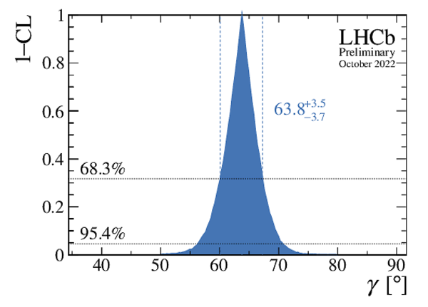
A combination of measurements sensitive to the $ C P$ violation angle $\gamma $ of the Cabibbo--Kobayashi--Maskawa unitarity triangle, to the charm mixing parameters that describe oscillations between $ D ^0$ and $\overline{ D } {}^0$ mesons, and to $ C P$ asymmetries in the $ D ^0 \rightarrow K ^+ K ^- $ and $ D ^0 \rightarrow \pi ^+ \pi ^- $ decays is performed. All relevant beauty and charm results obtained with the data collected with the LHCb detector at CERN's Large Hadron Collider to date are included. The charm mixing parameters are determined to be $ x = (0.398^{ +0.050}_{ -0.049})\% $ and $ y = (0.636^{ +0.020}_{ -0.019})\% $, the magnitude and phase of $ C P$ violation in charm mixing to be $ |q/p| = (0.995^{ +0.015}_{ -0.016}) $ and $\phi = (2.5 \pm 1.2)^\circ $, and the $ C P$ asymmetries in decay to be $ a_{ K ^+ K ^- }^{\textnormal{d}}$ = $ (9.0 \pm 5.7) \times 10^{-4}$ and $ a_{\pi ^+ \pi ^- }^{\textnormal{d}}$ = $ (24.0 \pm 6.2) \times 10^{-4}$ , with a correlation of $\rho=0.88$. The angle $\gamma $ is found to be $ (63.8^{ +3.5}_{ -3.7})^\circ $ and is the most precise determination from a single experiment.

Figures and captions

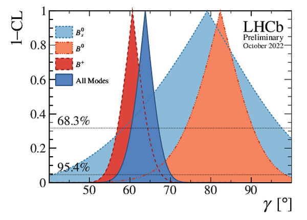
One dimensional profile likelihood scans of the $ 1-{\rm CL}$ distribution for $\gamma $ from the combination using inputs from $ B ^0_ s $ (light blue, dotted), $ B ^0$ (orange, dot-dashed), $ B ^+ $ mesons (red, dashed) and all species together (blue, solid).	gammac[..].pdf [16 KiB] HiDef png [433 KiB] Thumbnail [243 KiB] *.C file
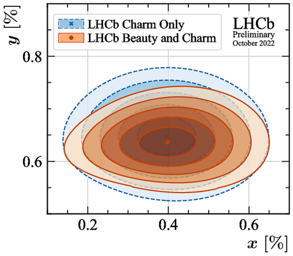
Two dimensional profile likelihood contours for (left) the charm mixing parameters $ x$ and $ y$ , and (right) the $ r_{D}^{K\pi}$ and $\delta_{D}^{K\pi}$ parameters. The blue contours (dashed) show the charm only inputs, the orange (solid) contours show the result of this combination. Contours are drawn out to $5\sigma$ and contain $68.3\%$, $95.4\%$, $99.7\%$, etc. of the distribution.	gammac[..].pdf [112 KiB] HiDef png [754 KiB] Thumbnail [366 KiB] *.C file
	gammac[..].pdf [136 KiB] HiDef png [693 KiB] Thumbnail [377 KiB] *.C file
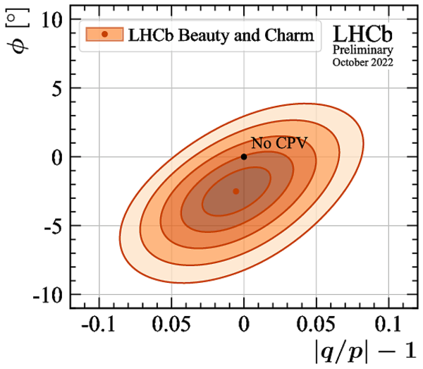
Two dimensional profile likelihood contours for (left) the $ C P$ asymmetries in the decay of the $ D ^0 \rightarrow K ^+ K ^- $ and $ D ^0 \rightarrow \pi ^+ \pi ^- $ channels, and (right) the $ \|q/p\|$ and $\phi$ parameters. The orange contours show the result of this combination, contours for the charm only inputs are indistinguishable so are not shown. Contours are drawn out to $5\sigma$ and contain $68.3\%$, $95.4\%$, $99.7\%$, etc. of the distribution.	gammac[..].pdf [125 KiB] HiDef png [485 KiB] Thumbnail [293 KiB] *.C file
	gammac[..].pdf [127 KiB] HiDef png [458 KiB] Thumbnail [270 KiB] *.C file
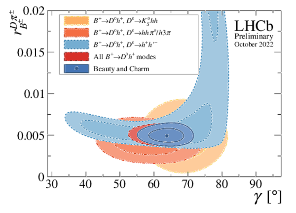
Profile likelihood contours for the components which contribute towards the $\gamma $ part of the combination, showing the breakdown of sensitivity amongst different sub-combinations of modes. The contours shown are the two-dimensional $1\sigma$ and $2\sigma$ contours which correspond to the areas containing 68.3% and 95.4% of the distribution.	gammac[..].pdf [22 KiB] HiDef png [467 KiB] Thumbnail [286 KiB] *.C file
	gammac[..].pdf [22 KiB] HiDef png [484 KiB] Thumbnail [294 KiB] *.C file
	gammac[..].pdf [22 KiB] HiDef png [501 KiB] Thumbnail [302 KiB] *.C file
	gammac[..].pdf [21 KiB] HiDef png [499 KiB] Thumbnail [303 KiB] *.C file
Profile likelihood contours for the charm decay and mixing parameters, showing the breakdown of sensitivity amongst different sub-combinations of modes. The contours indicate the 68.3% and 95.4% confidence regions.	gammac[..].pdf [19 KiB] HiDef png [469 KiB] Thumbnail [296 KiB] *.C file
	gammac[..].pdf [23 KiB] HiDef png [507 KiB] Thumbnail [290 KiB] *.C file
	gammac[..].pdf [32 KiB] HiDef png [714 KiB] Thumbnail [391 KiB] *.C file
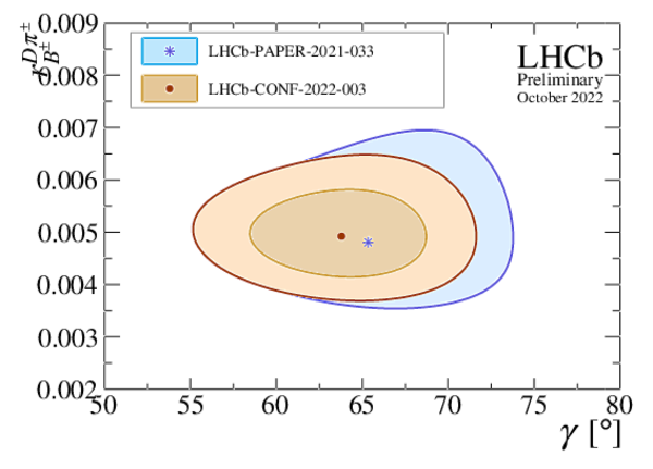
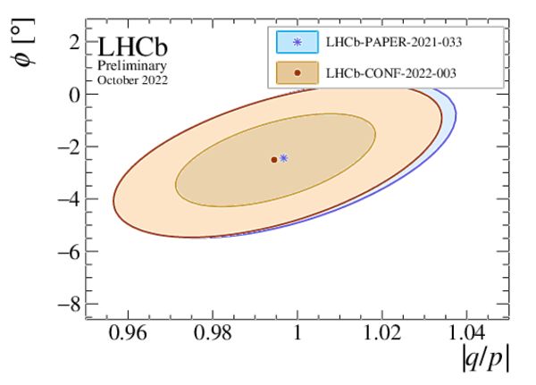
Two dimensional profile likelihood contours making a comparison between the previous combination \cite{LHCb-PAPER-2021-033} (blue) and the current one (brown). The contours shown are the two-dimensional $1\sigma$ and $2\sigma$ contours which correspond to areas containing 68.3% and 95.4% of the distribution.	gammac[..].pdf [16 KiB] HiDef png [299 KiB] Thumbnail [178 KiB] *.C file
	gammac[..].pdf [17 KiB] HiDef png [326 KiB] Thumbnail [195 KiB] *.C file
	gammac[..].pdf [17 KiB] HiDef png [352 KiB] Thumbnail [219 KiB] *.C file
	gammac[..].pdf [17 KiB] HiDef png [360 KiB] Thumbnail [220 KiB] *.C file
	gammac[..].pdf [17 KiB] HiDef png [346 KiB] Thumbnail [208 KiB] *.C file
	gammac[..].pdf [17 KiB] HiDef png [324 KiB] Thumbnail [197 KiB] *.C file
	gammac[..].pdf [16 KiB] HiDef png [342 KiB] Thumbnail [210 KiB] *.C file
One dimensional $ 1-{\rm CL}$ profile for $\gamma $ from all inputs used in the combination.	gammac[..].pdf [14 KiB] HiDef png [189 KiB] Thumbnail [139 KiB] *.C file
Two dimensional profile likelihood contours for the charm mixing parameters $ x$ and $ y$ . The blue (dashed) contours show the charm only inputs, the orange (solid) contours show the result of this combination. Contours are drawn out to $5\sigma$ and contain 68.3%, 95.4%, 99.7%, etc. of the distribution.	gammac[..].pdf [114 KiB] HiDef png [450 KiB] Thumbnail [266 KiB] *.C file
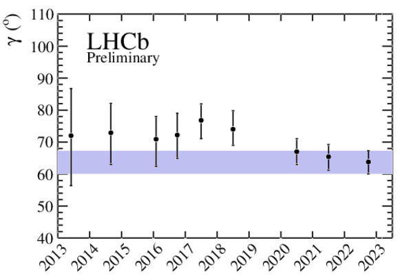
Evolution of published LHCb combination results for $\gamma $ , with the central values and $1\sigma$ uncertainties in black. The result presented in this note is the rightmost data point; its value and uncertainty are highlighted by the dashed blue line and band, respectively.	gamma_[..].pdf [14 KiB] HiDef png [167 KiB] Thumbnail [130 KiB] *.C file
Animated gif made out of all figures.	CONF-2022-003.gif Thumbnail

Tables and captions

Measurements used in the combination. Those that are new, or that have changed, since the previous combination \cite{LHCb-PAPER-2021-033} are highlighted in bold. The Run 1 and 2 took place from 2011 to 2012, corresponding to $1(2)\text{ fb} ^{-1} $ of integrated luminosity of proton-proton collisions at a centre-of-mass energy of $7(8)\text{ Te V} $, and from 2015 to 2018, corresponding to $6\text{ fb} ^{-1} $ at $13\text{ Te V} $, respectively. Measurements denoted by (*) include only a fraction of the Run 2 sample, corresponding to data taken in 2015 and 2016. Where multiple references are cited, measured values are taken from the most recent results, which include information from the others.	Table_1.pdf [97 KiB] HiDef png [217 KiB] Thumbnail [98 KiB] tex code
Auxiliary inputs used in the combination. Those highlighted in bold have changed since the previous combination \cite{LHCb-PAPER-2021-033}.	Table_2.pdf [97 KiB] HiDef png [83 KiB] Thumbnail [35 KiB] tex code
Confidence intervals and central values for each of the parameters of interest, computed using the Feldman-Cousins Plugin method \cite{Bodhisattva:2009uba}. Entries marked with an asterisk show where the scan has hit a physical boundary at the lower limit.	Table_3.pdf [95 KiB] HiDef png [279 KiB] Thumbnail [123 KiB] tex code
Confidence intervals and best-fit values for $\gamma $ when splitting the combination inputs by initial $B$ meson species, computed using the Feldman-Cousins Plugin method \cite{Bodhisattva:2009uba}.	Table_4.pdf [60 KiB] HiDef png [43 KiB] Thumbnail [20 KiB] tex code
Confidence intervals and best-fit values for $\gamma $ when splitting the combination inputs by time-dependent and time-integrated methods.	Table_5.pdf [61 KiB] HiDef png [31 KiB] Thumbnail [15 KiB] tex code
Reduced correlation matrix for the parameters of greater interest. Values smaller than $0.01$ are replaced with a - symbol.	Table_6.pdf [72 KiB] HiDef png [52 KiB] Thumbnail [23 KiB] tex code
Correlation matrix of the fit result. Values smaller than $0.01$ are replaced with a - symbol.	Table_7.pdf [81 KiB] HiDef png [53 KiB] Thumbnail [21 KiB] tex code
Correlation matrix for the $ B ^\pm \rightarrow D h^\pm $ , $ D\rightarrow K ^\pm \pi ^\mp \pi ^+ \pi ^- $ inputs.	Table_8.pdf [60 KiB] HiDef png [44 KiB] Thumbnail [22 KiB] tex code
Contributions to the total $\chi^2$ and the number of observables of each input measurement.	Table_9.pdf [83 KiB] HiDef png [264 KiB] Thumbnail [139 KiB] tex code