Feynman diagrams for $ B ^0_ s \rightarrow D_s^+ K^-$ decays (left) without and (right) with $ B ^0_ s $ -- $\overline{ B } {}^0_ s $ mixing.

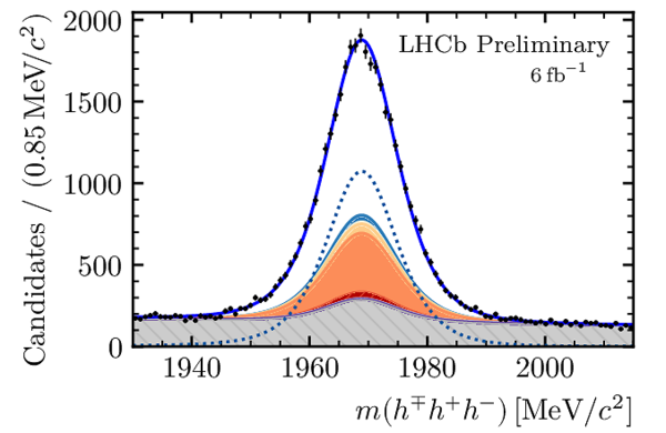
Distributions of the (left) $ D ^{\pm}_ s K^{\mp}$ and (right) $3h$ invariant masses for selected $D_s^\mp K^\pm$ candidates. In each plot, the contributions from all $ D ^-_ s $ final states and years of data taking are combined. The solid blue curve is the total result of the simultaneous fit. The dotted curve shows the $ B^0_s \rightarrow D_s^\mp K^\pm$ signal and the shaded stacked histograms show the different background contributions.

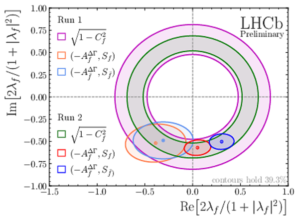
Representation of the $ C P$ -violating parameters in the $\mathrm{Im} \left[2\lambda_f/(1+|\lambda_f|^2)\right]$ vs $\mathrm{Re} \left[2\lambda_f/(1+|\lambda_f|^2)\right]$ cartesian plane.

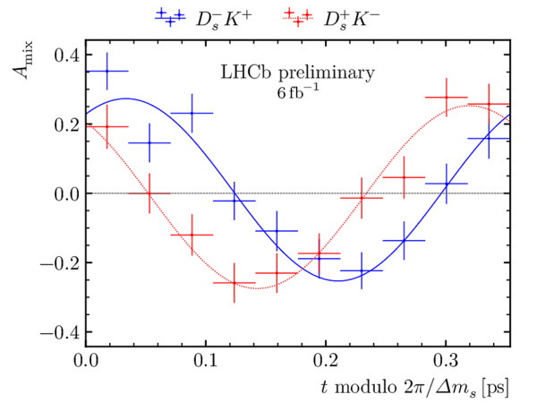
(Top) Decay-time distribution of $ B^0_s \rightarrow D_s^\mp K^\pm$ candidates obtained by the sPlot technique. (Bottom) $ C P$ -asymmetry for the (blue) $ D ^-_ s K^+$ and the (red) $ D ^+_ s K^-$ final states, folded into one mixing period, $2\pi/\Delta m_{ s } $. In both plots, the solid curve shows the result of the decay-time fit.

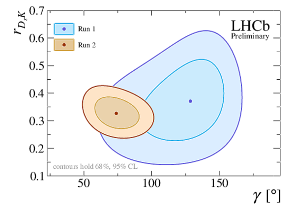
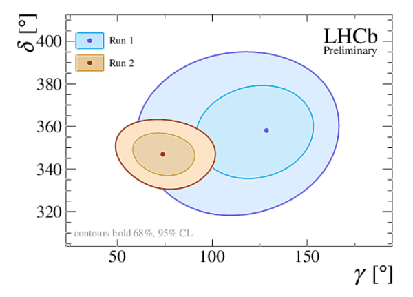
Profile likelihood contours of (top left) $ r_{D_sK}$ vs. $\gamma $ , and (top right) $\delta$ vs. $\gamma $ . The markers denote the best-fit values. The contours correspond to 68.3% CL (95.5% CL). The bottom plot shows $ 1-{\rm CL}$ for the angle $\gamma $ , together with the central value and the 68.3% CL interval as obtained from the frequentist method described in the text. The results with the Run 2 and Run 1 labels are from the present analysis and from Ref. [20], respectively.

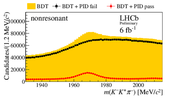
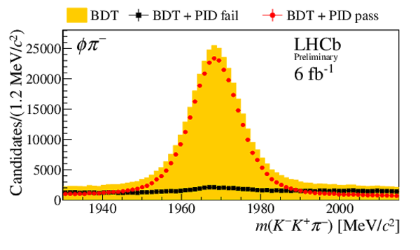
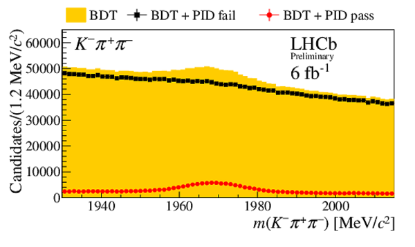
Invariant mass distribution $m(h^{-}h^{+}h^{\pm})$ after BDT selection (orange) and for candidates passing (red circles) or failing (black squares) the PID selection on the $ D ^-_ s $ candidate decay products. No PID requirements are applied to the companion kaon candidate. Distributions are shown for the final states (top left) $ D ^-_ s \rightarrow \phi\pi ^- $ , (top right) $ D ^-_ s \rightarrow K^{*0} K ^- $ , (middle left) $ D_s^- \rightarrow ( K ^- K ^+ \pi ^- )_{\text{nonresonant}}$, (middle right) $ D ^-_ s \rightarrow K ^- \pi ^+ \pi ^- $ , and (bottom) $ D ^-_ s \rightarrow \pi ^- \pi ^+ \pi ^- $ . These subsamples are defined by the invariant mass selections on the $K K$ and $K \pi$ systems given in Sec. 3.

The decay-time distribution of $ B^0_s \rightarrow D_s^\mp K^\pm$ signal candidates obtained using the sPlot technique. The dotted blue curve (left axis, arbitrary units) describes the decay rate. The solid orange curve (right axis, arbitrary units) describes the decay-time acceptance by which the decay rate is multiplied.

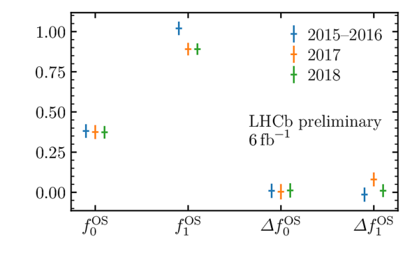
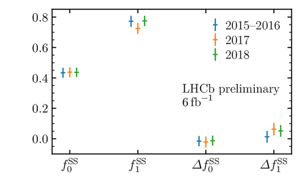
Flavour tagging calibration parameters for (left) the OS combination and (right) the SS combination obtained from the decay time fit to $ B^0_s \rightarrow D_s^- \pi^+$ . Uncertainties shown are statistical only, and are scaled by a factor of 10 for $f_{0}$ and $\Delta f_{0}$. These calibrations use a similar method to that described in Ref. [40], but use an updated selection and resolution determination for the analysis described here.

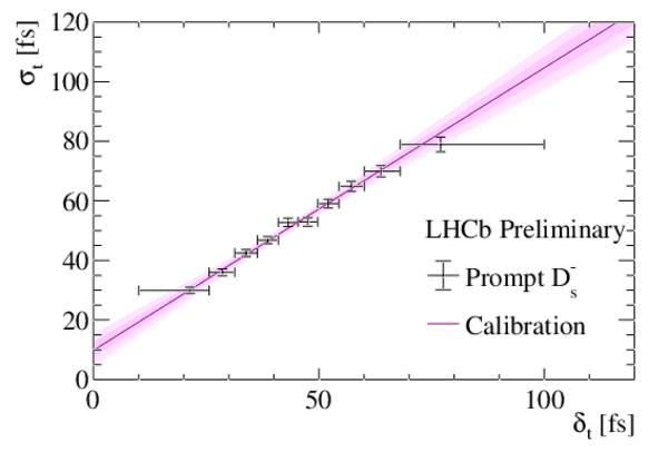
Measured decay-time resolution $\sigma_t$ as a function of the per-candidate decay-time uncertainty $\delta_t$ for prompt $D_s^{\mp}$ candidates combined with a random track. Data points are from the data collected in 2018 only. The solid line shows the linear fit to the data, as discussed in the text. The confidence intervals corresponding to one and two standard deviations of statistical uncertainty are indicated in magenta.

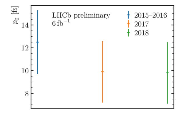
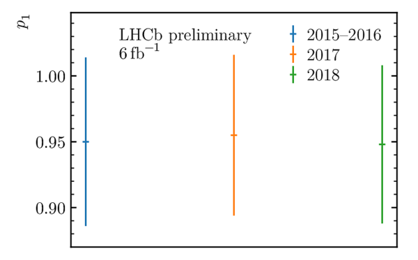
Decay-time resolution calibration parameters $p_0$ (left) and $p_1$ (right) used in the decay-time fit, obtained by combining the two Gaussian widths forming the core of the prompt $ D ^-_ s $ $\pi ^+$ decay-time distribution.

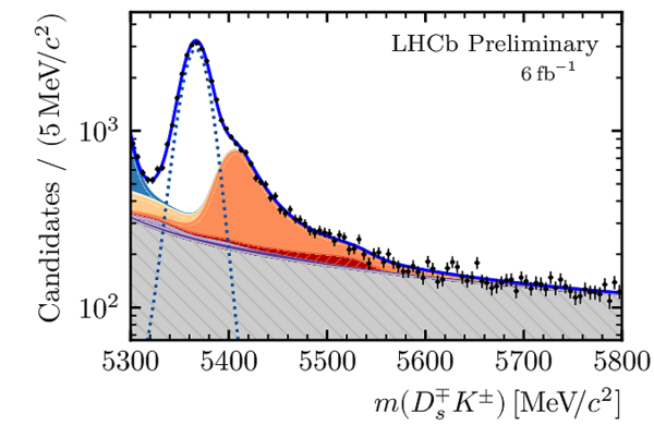
Distributions of the (left) $ D ^{\pm}_ s K^{\mp}$ and (right) $3h$ invariant masses for $ B^0_s \rightarrow D_s^\mp K^\pm$ final states, presented using a logarithmic scale on the vertical axis. In each plot, the contributions from all $ D ^-_ s $ final states and years of data taking are combined. The solid blue curve is the total result of the simultaneous fit. The dotted curve shows the $ B^0_s \rightarrow D_s^\mp K^\pm$ signal and the fully coloured stacked histograms show the different background contributions.

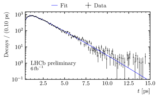
Decay-time distribution of $ B^0_s \rightarrow D_s^\mp K^\pm$ candidates obtained using the sPlot technique, with a logarithmic scale on the $y$ axis. The decay-time fit is overlaid.

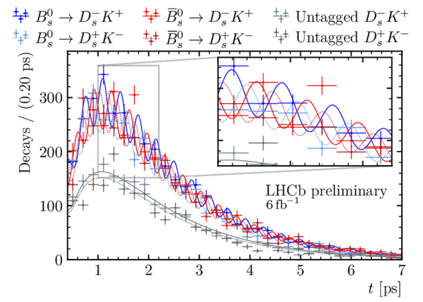
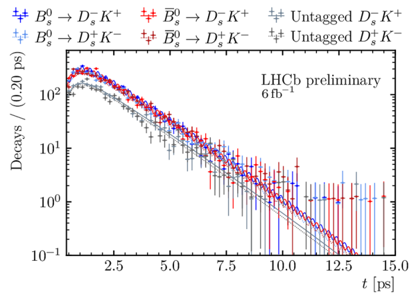
Decay-time distribution of signal $ B^0_s \rightarrow D_s^\mp K^\pm$ candidates split by final state and tagging category.

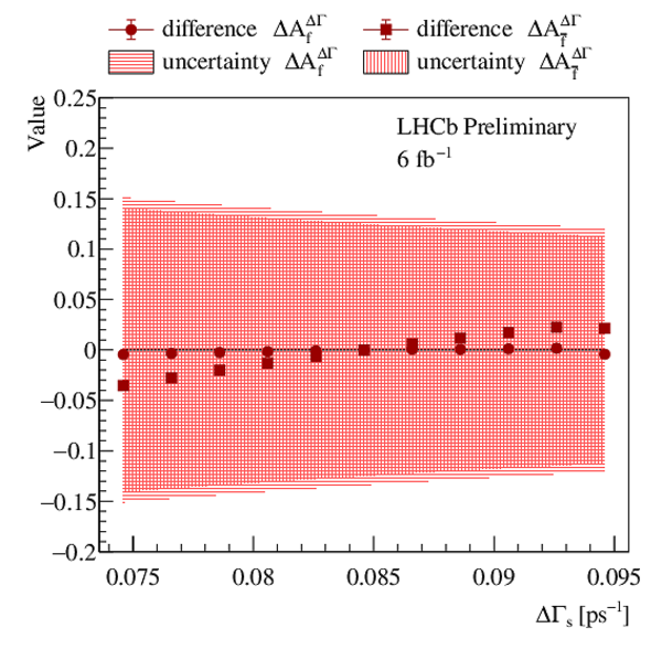
Dependence of the parameters $ A^{\Delta \Gamma}_f$ and $ A^{\Delta \Gamma}_{\bar{f}}$ on $\Delta\Gamma_{ s }$ . Red horizontally and vertically hatched bands represent the statistical uncertainty of the $ A^{\Delta \Gamma}_f$ and $ A^{\Delta \Gamma}_{\bar{f}}$ parameters, while circles (squares) denote the difference of the $ A^{\Delta \Gamma}_f$ ( $ A^{\Delta \Gamma}_{\bar{f}}$ ) parameter with respect to the baseline result.

Animated gif made out of all figures.

Values of the $ C P$ observables obtained from the fit to the decay-time distribution of $ B^0_s \rightarrow D_s^\mp K^\pm$ decays. The first uncertainty is statistical and the second is systematic.

Statistical correlation matrix of the $ C P$ observables. Other fit parameters have negligible correlations with the $ C P$ observables.

Systematic uncertainties on the $ C P$ observables, relative to the statistical uncertainties.

Correlation matrix of the total systematic uncertainties of the $ C P$ observables.