Side view of the LHCb spectrometer, with the two RICH detectors indicated

Invariant mass distribution for B$\rightarrow h^+h^-$ decays [3] in the LHCb data before the use of the RICH information (left), and after applying RICH particle identification (right). The signal under study is the decay B$^0\rightarrow\pi^+\pi^-$, represented by the turquoise dotted line. The contributions from different $b$-hadron decay modes (B$^0 \rightarrow$ K$\pi$ red dashed-dotted line, B$^0\rightarrow $3-body orange dashed-dashed line, B$_s \rightarrow$ KK yellow line, B$_s \rightarrow$ K$\pi$ brown line, $\Lambda_b \rightarrow$ pK purple line, $\Lambda_b \rightarrow$ p$\pi$ green line), are eliminated by positive identification of pions, kaons and protons and only the signal and two background contributions remain visible in the plot on the right. The grey solid line is the combinatorial background

RICH data-flow through the online system. Events selected by the L0 trigger are sent to the High Level Trigger (HLT) farm and, if they pass this trigger requirements, are sent to storage. A fraction of these events (typically 10%) is also sent to the monitoring farm. Online monitoring algorithms examine the data for irregularities and send messages to the slow-control (ECS) that can trigger automatic actions. Special triggers are sent directly to the calibration farm bypassing the High Level Trigger

Distribution of the midpoints in RICH 1 (left) and RICH 2 (right) after time alignment with pp collisions. The RMS deviations of the HPDs are approximately 1 ns

Spatial residuals demonstrating the resolution with which the light spots of the test pattern in RICH 1 are identified. The plot shows the distance from the measured light spot centre to the nearest test point. The dotted and solid lines are before and after the calibration respectively, along the $x$ direction (left) and along $y$ (right) of the anode plane, projected on the photocathode plane. The solid line is the Gaussian fit

Spatial residuals demonstrating the resolution with which the light spots of the test pattern in RICH 2 are identified. The plot shows the distance from the measured light spot centre to the nearest test point. The dotted and solid lines are before and after the calibration respectively. Most of the photodetectors of RICH 2 are in a region free from magnetic field residual values (region around $x$=0 of the dotted histogram). Where these are different from zero, the distorsions induced are visible in the two satellite peaks of opposite sign (the magnetic field changes sign in the upper and lower part of the photodetector matrix plane). The left plot is the measurement along the $x$, the right plot along $y$ of the anode plane, projected on the photocathode plane. The solid line is the Gaussian fit

$\Delta\theta_C$ plotted as a function of the azimuthal angle $\phi$ and fitted with $\theta_{x} \cos(\phi) + \theta_{y}\sin(\phi)$, for one side of the RICH 2 detector. The left-hand plot is prior to alignment, and shows a dependency of the angle $\theta_{C}$ on the angle $\phi$. The right-hand plot is after the alignment correction, and $\Delta \theta_{C}$ is uniform in $\phi$

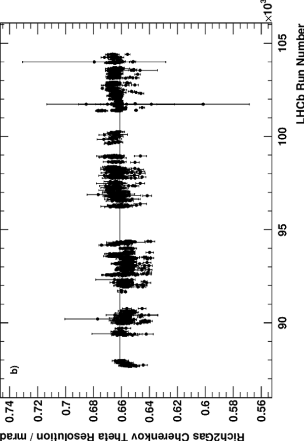
The Cherenkov angular resolution (c.f. Sect. 4.2), after all corrections have been applied, as a function of run number. a) for RICH 1 and b) for RICH 2. The period of time covered on the x-axis corresponds to about 8 months of running

Single photoelectron resolution for the RICH 1 (left) and RICH 2 (right) gases, as measured in data for high momentum charged particles. The red line describes the background as determined from the fit using a polynomial function together with the Gaussian for the signal

Single photoelectron resolution for the aerogel as measured in 2011 data with the pp$\rightarrow$pp$\mu^+\mu^-$ events. The red line describes the background as determined from the fit using a polynomial function together with two Gaussians for the signal

Distribution of $\Delta \theta_C$ for C$_4$F$_{10}$. This plot is produced from kaons and pions from tagged D$^0 \rightarrow$ K$^- \pi^+$ decays in data selected with the criteria described in the text

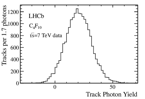
Individual track photon yield distributions for the C$_4$F$_{10}$ (left) and CF$_4$ (right) radiators. The plot is produced from kaons and pions from tagged D$^0 \rightarrow$ K$^- \pi^+$ decays in data selected with the criteria described in the text

Distribution of the number of pixel hits per event in (a) RICH 1 and (b) RICH 2. An example of a typical LHCb event as seen by the RICH detectors, is shown below the distributions. The upper/lower HPD panels in RICH 1 and the left/right panels in RICH 2 are shown separately

Reconstructed Cherenkov angle as a function of track momentum in the $\rm C_{4}F_{10}$ radiator

Invariant mass distributions of the (a) K$^{0}_{S}$, (b) $\Lambda$ and (c) D$^{0}$ calibration samples. The best fit probability-density-function (pdf), describing both background and signal, is superimposed in blue

Distribution of $\rm\Delta log \mathcal{L}(K - \pi)$ against $\rm\Delta log \mathcal{L}(p - \pi)$ for (a) pions, (b) kaons and (c) protons extracted from the control samples

Kaon identification efficiency and pion misidentification rate measured on data as a function of track momentum. Two different $\rm\Delta log \mathcal{L}(K-\pi)$ requirements have been imposed on the samples, resulting in the open and filled marker distributions, respectively

Kaon identification efficiency and pion misidentification rate measured using simulated events as a function of track momentum. Two different $\rm\Delta log \mathcal{L}(K-\pi)$ requirements have been imposed on the samples, resulting in the open and filled marker distributions, respectively

Proton identification efficiency and pion misidentification rate measured on data as a function of track momentum. Two different $\rm\Delta log \mathcal{L}(p-\pi)$ requirements have been imposed on the samples, resulting in the open and filled marker distributions, respectively

Proton identification efficiency and kaon misidentification rate measured on data as a function of track momentum. Two different $\rm\Delta log \mathcal{L}(p-K)$ requirements have been imposed on the samples, resulting in the open and filled marker distributions, respectively

Pion misidentification fraction versus kaon identification efficiency as measured in 7 TeV LHCb collisions: (a) as a function of track multiplicity, and (b) as a function of the number of reconstructed primary vertices. The efficiencies are averaged over all particle momenta

Animated gif made out of all figures.

Comparison of photoelectron yields (N$_{\rm pe}$) determined from D$^* \rightarrow$D$^0\pi^+$ decays in simulation and data, and pp $\rightarrow$ pp $\mu^+ \mu^-$ events in data, using the selections and methods described in the text