A schematic representation of an R-type and a $\rm{\phi}$-type sensor, with the routing lines orientated perpendicular and parallel to the silicon strips, respectively.

Currents measured in the VELO for each sensor as a function of time (bottom). The luminosity delivered to LHCb and the average sensor temperature is shown over the same time scale (middle and top). Increases in the delivered luminosity are matched by increases in the sensor currents. The mean measured current agrees well with the prediction from simulation, which is described in Sect.2.4. The mean measured value excludes sensors that are surface-current dominated.

The current versus temperature for two VELO sensors operated at the nominal $150\rm{ V}$ bias. Before irradiation there is a small exponential component for the sensor shown in figure a), while that shown in figure b) is dominated by the non-temperature dependent surface current contribution. After irradiation, a large exponential component is seen for both sensors. These sensors are now bulk current dominated and the surface current has largely been annealed.

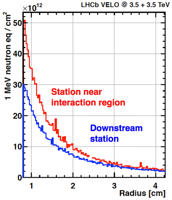
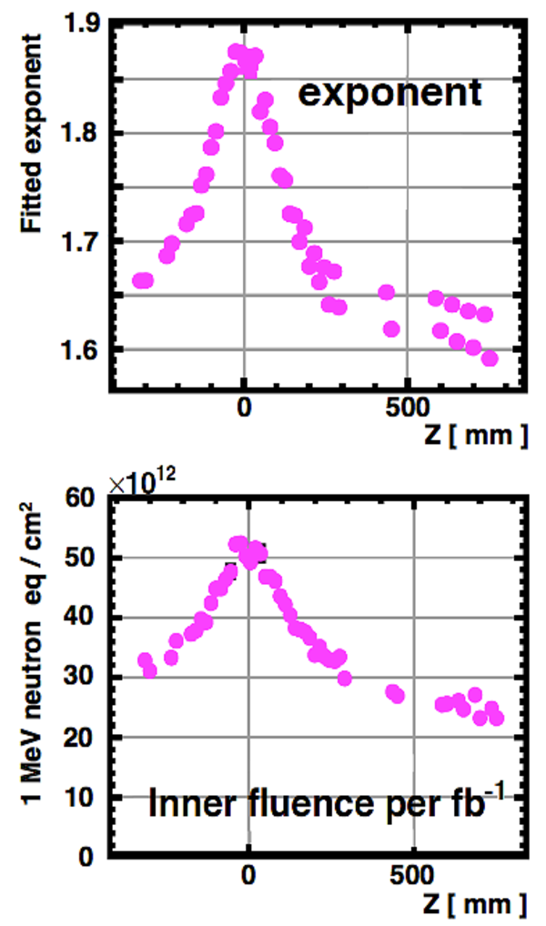
a) The fluence from $\rm{1 fb^{-1}}$ of integrated luminosity versus radius for two VELO sensors, as seen in simulated proton-proton collisions at a $7$ TeV centre-of-mass energy. Top b) In each sensor, the fluence as a function of radius is fitted with the function $\rm{Ar^{k}}$. The fitted exponent, ${\rm k}$, is shown as a function of the sensor $z$-coordinate, where $z$ is the distance along the beam-axis that a sensor is from the interaction region. The distribution of the fluence across the sensor is seen to become flatter with increasing distance from the interaction region. Bottom b) The fluence at the innermost radius of the sensor against the sensor $z$-coordinate.

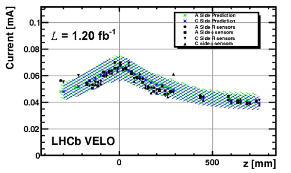
The leakage current against sensor $z$-coordinate after $\rm{1.20 fb^{-1}}$ of integrated luminosity, normalised to $0 ^{\circ}{\rm C}$. The data is in agreement with predictions, represented by the shaded region. The two VELO halves are referred to as the A and C sides of the VELO.

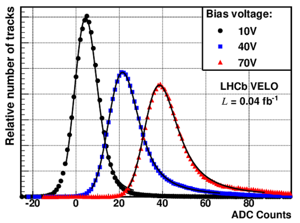
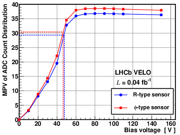
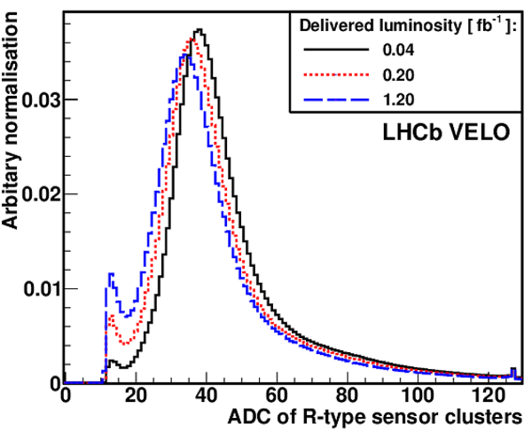
a) The pedestal subtracted ADC distributions for an R-type sensor at three example bias voltages. b) The MPV of the fit to the ADC distribution vs. bias voltage. The dashed lines represent the ADC that is $80\%$ of the plateau value, and the corresponding EDV.

a) The EDV against sensor radius for an $\rm {\it{n^+}} -on -{\it{n}}$ {} type sensor for each of the CCE scans. The dashed line shows the mean EDV across all radius regions prior to sensor irradiation, where some $0 \rm{fb^{-1}}$ data points are not present due to low statistics. b) A similar plot for the $\rm {\it{n^+}} -on -{\it{p}}$ {}, $\phi$-type sensor. The minimum EDV is $\rm{\mathord{\sim} 40 V}$, which is significantly higher than the minimum at $\rm{\mathord{\sim} 20 V}$ observed for the $\rm {\it{n^+}} -on -{\it{n}}$ {} type sensor.

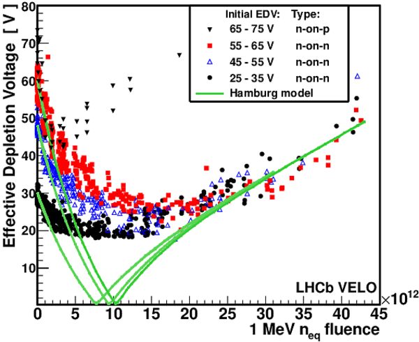
The EDV against fluence for VELO sensors of various initial EDV. The EDV from data is compared to depletion voltages predicted by the Hamburg model, with good agreement observed prior to, and after sensor type-inversion.

The inverse of the sensor noise against bias voltage for a particular $\rm {\it{n^+}} -on -{\it{n}}$ {} and $\rm {\it{n^+}} -on -{\it{p}}$ {} type sensor, for two values of integrated luminosities. The C-V scan measured initial depletion voltages are shown by the dashed lines.

The CFE for an R-type $\rm {\it{n^+}} -on -{\it{n}}$ {} sensor as a function of sensor radius for a) different amounts of delivered luminosity and b) several different bias voltages.

a) The layout of the second metal layer routing lines on an R-type sensor. The darker regions represent the presence of routing lines, and the lighter regions their absence. b) The CFE shown in small spatial regions of an R-type sensor.

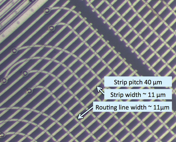
A photograph of the innermost region of an R-type sensor. Strips run from the bottom-left to the top-right. Each strip is connected to a routing line orientated perpendicularly to the strip.

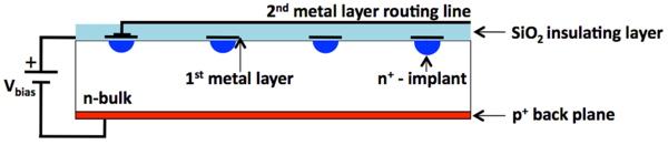
A schematic cross-section of a portion of an R-type sensor, showing the relative position of the two metal layers used to carry the readout signals in $\rm {\it{n^+}} -on -{\it{n}}$ {} type sensors. The $n^{+}$ implants and strips (into the page) run perpendicularly to the routing lines (left to right). For clarity the routing line of just one strip is shown.

The CFE as a function of the distance between the particle intercept and the nearest routing line, for several bins of the distance between the particle intercept and closest strip edge.

For R-type sensors: a) The ADC spectrum of all clusters seen for three different integrated luminosities. The limit at $10$ ADC counts is imposed by the clustering thresholds. b) The fraction of reconstructed clusters that are induced on routing lines as a function of the distance to the nearest routing line and strip. This is determined from the number of track intercepts for which the inner strip associated to the nearest routing line has a $1$ strip cluster with less than $35$ ADC counts.

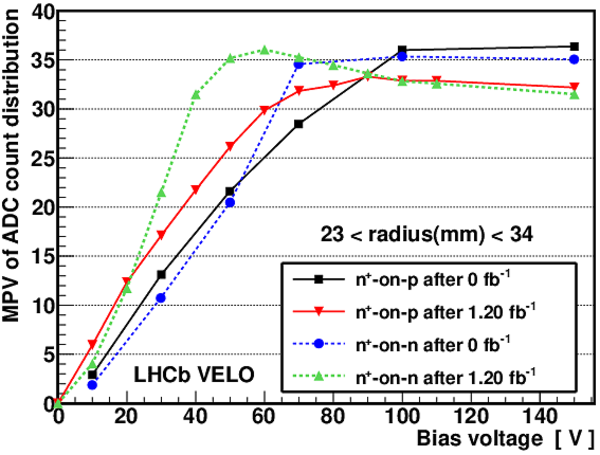
a) The CFE as a function of the distance between the particle intercept and the nearest routing line and strip edge, compared for an $\rm {\it{n^+}} -on -{\it{n}}$ {} and $\rm {\it{n^+}} -on -{\it{p}}$ {} sensor. b) The MPV vs. bias voltage for an $\rm {\it{n^+}} -on -{\it{n}}$ {} and $\rm {\it{n^+}} -on -{\it{p}}$ {} sensor.

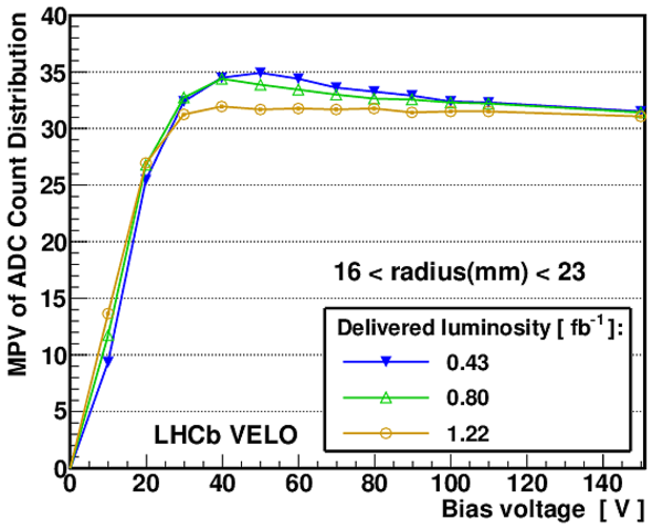
The MPV against bias voltage for an R-type sensor at three values of delivered luminosity. The sensor region has been identified as having type inverted in the $1.20 \rm{fb^{-1}}$ scan, in which the MPV dependence on voltage is no longer present.

Animated gif made out of all figures.

The VELO sensor design parameters. The sensor position along the beam axis is given relative to the beam interaction region.

The effective band gap, $E_{g}$, measured following various amounts of delivered luminosity. The first uncertainty is statistical and the second is systematic.