From Ref. [1]: (top left) a photograph of one side of the VELO, taken during assembly, showing the silicon sensors and readout hybrids; (top right) a schematic of both an $r$ and $\phi$ sensor, showing the sensor strips and routing lines; and (bottom) schematics showing the cross section of the $xz$ plane at $y=0$, where the $r(\phi)$ sensors are shown with solid blue (dashed red) lines, and an $xy$ view of overlapping sensors in the closed position. { N.b.}, the modules at positive (negative) $x$ are known as the left or A-side (right or C-side).

Reconstructed SVs in the Run 2 data sample showing the $xy$ plane integrated over $z$ within the region of the VELO that contains sensor modules. The left (right) panel shows the central (forward) VELO region. The bins are $0.1 mm \times0.1 mm $ in size.

Reconstructed SVs in the Run 1 data sample showing the $zr$ plane integrated over $\phi$, where a positive (negative) $r$ value denotes that the SV is closest to material in the right (left) half of the VELO. The bins are $0.1 mm \times1 mm $ in size. { N.b.}, the inner-most RF-foil region is nearly semi-circular in the $xy$ plane, which results in sharp edges at smaller $r$ values; however, at large $|y|$ values, the RF-foil is flat producing SVs at larger values of $r$ which can easily be mistaken as background in the $zr$ projection shown here.

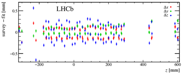
Differences in the sensor locations relative to the survey specifications. The observed deviations are known from VELO alignment studies and accounted for during reconstruction.

Comparison between the RF-foil map at $y=0 mm $ and the description in LHCb simulation.

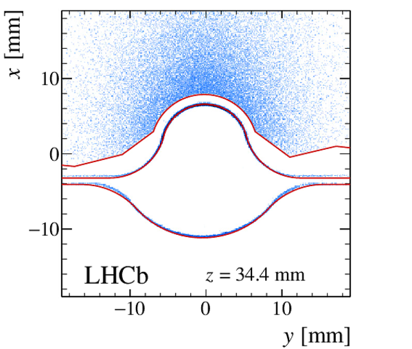
Example comparisons between the (filled bins) reconstructed SV locations and (red lines) the material map for: (top) $x$ versus $z$ near $y=0 mm $; (middle) same as the top but zoomed in on the ${0 < z < 100 mm }$ region; (bottom left) $x$ versus $y$ near the left-half $r$ sensor at $z=34.4 mm $; and (bottom right) $x$ versus $y$ near the right-half $\phi$ sensor at $z=49.3 mm $. For visual clarity: in the top panel, the red vertical lines denote the center of each sensor, while in the bottom panels only the edges of the sensors are shown; and in all panels, only the nominal RF-foil position is shown; { i.e.} the red RF-foil curves do not display its thickness.

The normalized photon conversion $p$-value distribution obtained using a subsample of data from an LHCb long-lived dark-photon search [8]. The data are consistent with the photon-conversion hypothesis. Some example dark-photon distributions are also shown for lifetimes of 1 and 10 ps, showing good separation between potential exotic signals and photon conversions.

Animated gif made out of all figures.