Fit to the $ K ^+ \pi ^- K ^- \pi ^+ $ mass distribution of selected candidates. The fit model (dashed pink curve) includes a signal component that has two Gaussian components corresponding to the $ B ^0_s$ and $ B ^0$ decays. The background is described as an exponential component (dotted blue) plus the parametrization indicated in the text (dash-dotted green).

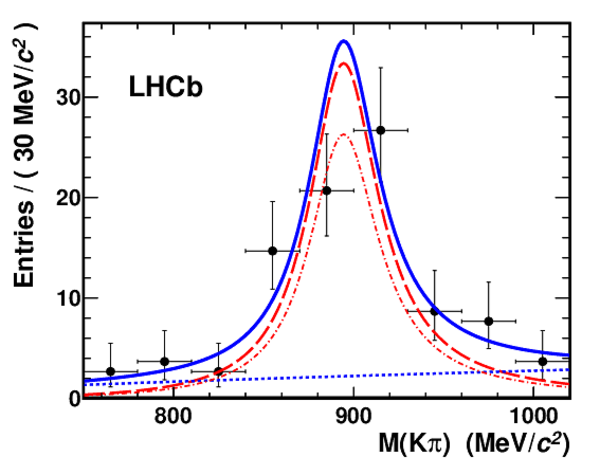
Background subtracted $K^+\pi^-$ and $K^-\pi^+$ combinations for selected candidates within a $\pm$50 $ {\mathrm{ Me V /}c^2}$ window of the $ B ^0_s$ mass. The solid blue line shows the projection of the 2D fit model described in the text, indicating the $ K ^{*0}$ $\overline{ K }{} ^{*0}$ yield (dashed-dotted red line) and a nonresonant component (blue dotted line), assumed to be a linear function times the two-body phase space. The dashed red line indicates the overall $ B ^0_s \rightarrow K ^{*0} X$ contribution.

Fit to the mass distribution of selected $ B ^0 \rightarrow { J \mskip -3mu/\mskip -2mu\psi \mskip 2mu} K ^{*0} $ events. The dashed red curve is the Gaussian component for the $ B $ signal. The green dashed-dotted line accounts for partially reconstructed $ B\rightarrow J/\psi X$ (see Eq. 2). The pink hatched region accounts for a possible $ B ^0_s \rightarrow { J \mskip -3mu/\mskip -2mu\psi \mskip 2mu} \phi$ contamination, parametrized as a sum of two Crystal-Ball functions [20]. The combinatorial background is parametrized as an exponential and indicated as a blue dotted line.

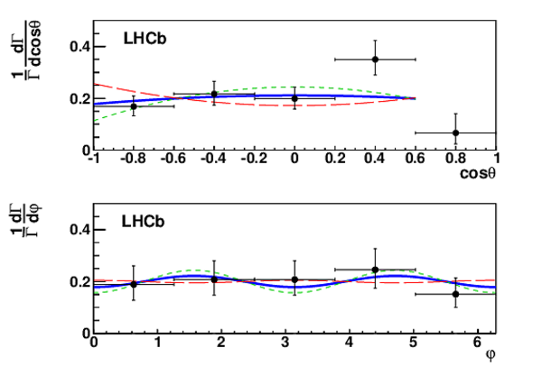
$\cos\theta$ (above) and $\varphi$ (below) acceptance corrected distributions for events in the narrow window around the $ B ^0_s$ mass. The blue line is the projection of the fit model given by Eq. 3 for the measured values of the parameters $f_L$, $f_{\parallel}$ and $\delta_{\parallel}$. The dotted lines indicate $\pm 1\sigma$ variation of the $f_L$ central value.

Animated gif made out of all figures.

Fitted values of the model parameters for the mass spectrum, as described in the text. $N_s$ and $N_d$ are the number of events for the $ B ^0_s$ and $ B ^0$ signals, $\mu_s$ is the fitted mass value for the $ B ^0_s$ signal and $\sigma$ is the Gaussian width. The mass difference between $ B ^0_s$ and $ B ^0$ was fixed to its nominal value [4]. $N_{b}$ is the number of background events in the full mass range (4900-5800 $ {\mathrm{ Me V /}c^2}$ ), and $c_{b}$ is the exponential parameter in the fit. $M_p$, $\sigma_p$ and $k_p$ are the parameters of Eq. (1). Finally, $f_{p}$ is the fraction of the background associated with Eq. (1).

Selection and trigger efficiencies obtained from simulation. The observed yield found for the signal and control channels in the full mass range are also indicated. The efficiency errors are statistical, derived from the size of the simulated samples.

Estimated systematic error sources in the $\cal B \left( B ^0_s \rightarrow K ^{*0} \overline{ K }{} ^{*0} \right)$ measurement.