Absolute luminosity measurements with the LHCb detector at the LHC

Information

LHCb-PAPER-2011-015
CERN-PH-EP-2011-157
arXiv:1110.2866 [PDF]

(Submitted on 13 Oct 2011)
JINST 7 P01010
Inspire 939619

Tools

Abstract

Absolute luminosity measurements are of general interest for colliding-beam experiments at storage rings. These measurements are necessary to determine the absolute cross-sections of reaction processes and are valuable to quantify the performance of the accelerator. Using data taken in 2010, LHCb has applied two methods to determine the absolute scale of its luminosity measurements for proton-proton collisions at the LHC with a centre-of-mass energy of 7 TeV. In addition to the classic "van der Meer scan" method a novel technique has been developed which makes use of direct imaging of the individual beams using beam-gas and beam-beam interactions. This beam imaging method is made possible by the high resolution of the LHCb vertex detector and the close proximity of the detector to the beams, and allows beam parameters such as positions, angles and widths to be determined. The results of the two methods have comparable precision and are in good agreement. Combining the two methods, an overall precision of 3.5 in the absolute luminosity determination is reached. The techniques used to transport the absolute luminosity calibration to the full 2010 data-taking period are presented.

Figures and captions

A sketch of the VELO, including the two Pile-Up stations on the left. The VELO sensors are drawn as double lines while the PU sensors are indicated with single lines. The thick arrows indicate the direction of the LHC beams (beam 1 going from left to right), while the thin ones show example directions of flight of the products of the beam-gas and beam-beam interactions.	Fig01.pdf [29 KiB] HiDef png [129 KiB] Thumbnail [86 KiB] *.C file
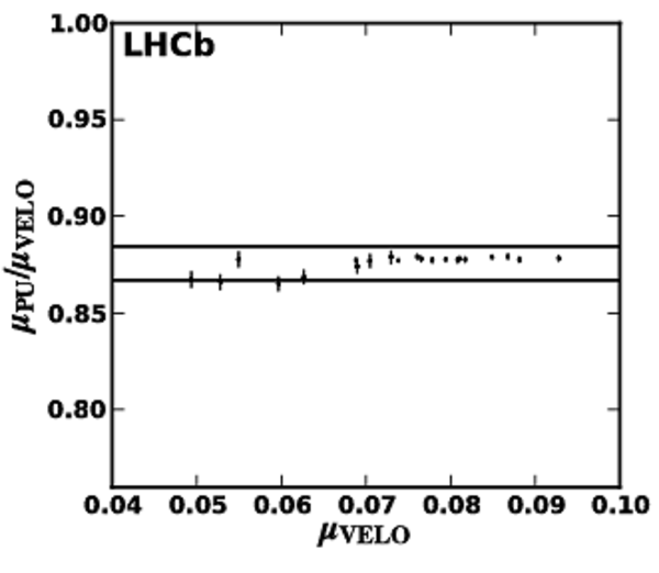
Ratio between $ {\mu^{}_{\mathrm{\mathrm{vis}}}}$ values obtained with the zero-count method using the number of hits in the PU and the track count in the VELO versus $ {\mu^{}_{\mathrm{VELO}}} $. The deviation from unity is due to the difference in acceptance. The left (right) panel uses runs from the beginning (end) of the 2010 running period with lower (higher) values of $ {\mu^{}_{\mathrm{VELO}}}$ . The horizontal lines indicate a $\pm1$% variation.	Fig02a.pdf [14 KiB] HiDef png [76 KiB] Thumbnail [59 KiB] *.C file
	Fig02b.pdf [84 KiB] HiDef png [110 KiB] Thumbnail [85 KiB] *.C file
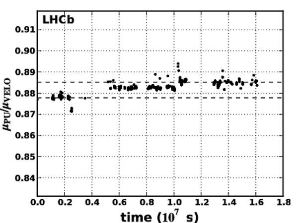
Ratio between $ {\mu^{}_{\mathrm{\mathrm{vis}}}}$ values obtained with the zero-count method using the number of hits in the PU and the track count in the VELO as a function of time in seconds relative to the first run of LHCb in 2010. The period spans the full 2010 data taking period (about half a year). The dashed lines show the average value of the starting and ending periods (the first and last 25 runs, respectively) and differ by $\approx1$%. The changes in the average values between the three main groups ($t < 0.4\times 10^7$ s, $0.4\times 10^7 < t < 1.2\times 10^7$ s, $t > 1.2\times 10^7$ s) coincide with known maintenance changes to the PU system. The upward excursion near $1.05 \times 10^7$ s is due to background introduced by parasitic collisions located at 37.5 m from the nominal IP present in the bunch filling scheme used for these fills to which the two counters have different sensitivity. The downward excursion near $0.25 \times 10^7$ s is due to known hardware failures in the PU (recovered after maintenance). The statistical errors are smaller than the symbol size of the data points.	Fig03.pdf [22 KiB] HiDef png [84 KiB] Thumbnail [86 KiB] *.C file
Evolution of the average number of interactions per crossing at the nominal beam position during the October scans. In the first (second) scan the parameters at the nominal beam position were measured three (four) times both during the $\Delta_x$ scan and the $\Delta_y$ scan. The straight line is a fit to the data. The luminosity decay time is 46 hours.	Fig04.pdf [12 KiB] HiDef png [47 KiB] Thumbnail [25 KiB] *.C file
Number of interactions per crossing summed over the twelve colliding bunches versus the separations $\Delta_x$ (top), $\Delta_y$ (bottom) in October. The first (second) scan is represented by the dark/blue (shaded/red) points and the solid (dashed) lines. The spread of the mean values and widths of the distributions obtained individually for each colliding pair are small compared to the widths of the VDM profiles, so that the sum gives a good illustration of the shape. The curves represent the single Gaussian fits to the data points described in the text.	Fig05.pdf [44 KiB] HiDef png [258 KiB] Thumbnail [163 KiB] *.C file
Cross-sections without correction for the FBCT offset for the twelve bunches of the October VDM fill (data points). The lines indicate the results of the fit as discussed in the text. The upper (lower) set of points is obtained in the first (second) scan.	Fig06.pdf [16 KiB] HiDef png [103 KiB] Thumbnail [67 KiB] *.C file
Average number of interactions ( $ {\mu^{}_{\mathrm{VELO}}}$ ) versus the centre of the luminous region summed over the twelve colliding bunches and measured during the length scale scans in $x$ (left) and in $y$ (right) taken in October. The points are indicated with small horizontal bars, the statistical errors are smaller than the symbol size. The straight-line fit is overlaid.	Fig07a.pdf [10 KiB] HiDef png [89 KiB] Thumbnail [55 KiB] *.C file
	Fig07b.pdf [10 KiB] HiDef png [88 KiB] Thumbnail [57 KiB] *.C file
Centre of the luminous region reconstructed with VELO tracks versus the position predicted by the LHC magnet currents. The points are indicated with small horizontal bars, the statistical errors are smaller than the symbol size. The points are fitted to a linear function. The slope calibrates the common length scale.	Fig08a.pdf [7 KiB] HiDef png [95 KiB] Thumbnail [61 KiB] *.C file
	Fig08b.pdf [7 KiB] HiDef png [91 KiB] Thumbnail [59 KiB] *.C file
Contours of the distribution of the $x$-$y$ coordinates of the luminous region. The contour lines show the values at multiples of 10% of the maximum. The points represent the $y$-coordinates of the centre of the luminous region in different $x$ slices. They are fitted with a linear function.	Fig09.pdf [10 KiB] HiDef png [175 KiB] Thumbnail [111 KiB] *.C file
Movement of the centre of the luminous region in $z$ during the first scan in $x$ taken in October.	Fig10.pdf [9 KiB] HiDef png [50 KiB] Thumbnail [29 KiB] *.C file
Primary vertex resolution $\sigma_{\mathrm{res}}$ in the transverse directions $x$ (full circles) and $y$ (open circles) for beam-beam interactions as a function of the number of tracks in the vertex, $ N_{\mathrm{Tr}}$ . The curves are explained in the text.	Fig11.pdf [23 KiB] HiDef png [139 KiB] Thumbnail [72 KiB] *.C file
The $z$ dependence of the resolution correction factor $ F_{z}$ in $x$ (full circles) and $y$ (open circles) for beam 1-gas (left) and beam 2-gas (right) interactions.	Fig12a.pdf [20 KiB] HiDef png [120 KiB] Thumbnail [66 KiB] *.C file
	Fig12b.pdf [19 KiB] HiDef png [110 KiB] Thumbnail [60 KiB] *.C file
Positions of reconstructed beam-gas interaction vertices for $ {\mathsf{be}}$ (black points) and $ {\mathsf{eb}}$ (grey points) crossings during Fill 1104. The measured beam angles $\alpha_{1,2}$ and offsets $\delta_{1,2}$ at $z=0$ in the horizontal (top) and vertical (bottom) planes are shown in the figure.	Fig13.png [155 KiB] HiDef png [84 KiB] Thumbnail [33 KiB] *.C file
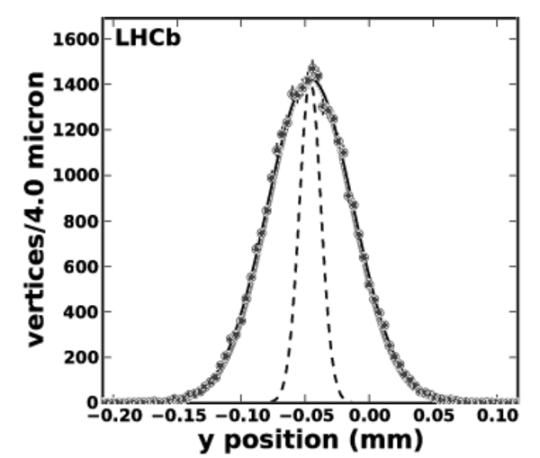
Distributions of the vertex positions of beam-gas events for beam 1 (top) and beam 2 (bottom) for one single bunch pair (ID 2186) in Fill 1104. The left (right) panel shows the distribution in $x$ ($y$). The Gaussian fit to the measured vertex positions is shown as a solid black curve together with the resolution function (dashed) and the unfolded beam profile (shaded). Note the variable scale of the horizontal axis.	Fig14a.pdf [17 KiB] HiDef png [200 KiB] Thumbnail [139 KiB] *.C file
	Fig14b.pdf [17 KiB] HiDef png [199 KiB] Thumbnail [140 KiB] *.C file
	Fig14c.pdf [15 KiB] HiDef png [198 KiB] Thumbnail [138 KiB] *.C file
	Fig14d.pdf [15 KiB] HiDef png [194 KiB] Thumbnail [133 KiB] *.C file
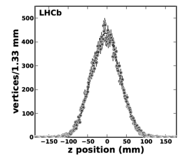
Distributions of vertex positions of $pp$ interactions for the full fill duration (left) and for a 900 s period in the middle of the fill (right) for one colliding bunch pair (ID 2186) in Fill 1104. The top, middle and bottom panels show the distributions in $x$, $y$ and $z$, respectively. The Gaussian fit to the measured vertex positions is shown as a solid black curve together with the resolution function (dashed) and the unfolded luminous region (shaded). Owing to the good resolution the shaded curves are close to the solid curves and are therefore not clearly visible in the figures. The fit to the $z$ coordinate neglects the vertex resolution. Note the variable scale of the horizontal axis.	Fig15a.pdf [20 KiB] HiDef png [215 KiB] Thumbnail [143 KiB] *.C file
	Fig15b.pdf [19 KiB] HiDef png [197 KiB] Thumbnail [128 KiB] *.C file
	Fig15c.pdf [18 KiB] HiDef png [212 KiB] Thumbnail [143 KiB] *.C file
	Fig15d.pdf [19 KiB] HiDef png [214 KiB] Thumbnail [143 KiB] *.C file
	Fig15e.pdf [21 KiB] HiDef png [195 KiB] Thumbnail [114 KiB] *.C file
	Fig15f.pdf [19 KiB] HiDef png [213 KiB] Thumbnail [121 KiB] *.C file
Comparison of the prediction for the luminous region width from measurements based on beam-gas events of individual bunches which are part of a colliding bunch pair with the direct measurement of the luminous region width for these colliding bunches. The panels on the left show the results for bunches in the fills with $\beta^* = 2$ m optics used in this analysis, the right panels show four colliding bunches in a fill taken with $\beta^* = 3.5$ m optics. The fill and bunch numbers are shown on the vertical axis. The vertical dotted line indicates the average and the solid lines the standard deviation of the data points. The lowest point indicates the weighted average of the individual measurements; its error bar represents the corresponding uncertainty in the average. The same information is given above the data points. The fills with the $\beta^* = 3.5$ m optics are not used for the analysis due to the fact that larger uncertainties in the DCCT calibration were observed.	Fig16.pdf [20 KiB] HiDef png [321 KiB] Thumbnail [218 KiB] *.C file
Left: the dependence of the length of the luminous region $\sigma_{\otimes\mathrm{z}}^{}$ on the single bunch length $\sigma_z$ under the assumption that both beams have equal length bunches. The dotted line shows the $\sqrt{2}$ behaviour expected in the absence of a crossing angle. The solid black line shows the dependence for equal transverse beam sizes $\sigma_x = 0.045$ mm, the shaded region shows the change for $\rho = 1.2$ keeping the average size constant. Right: the dependence of the luminosity reduction factor $C_{\mathrm{\alpha }}$ on the transverse width of the beam $\sigma_x$ for a value of $\sigma_{\otimes\mathrm{z}}^{} = 35$ mm. The solid line shows the full calculation for $\rho = 1$ (equal beam widths) with the shaded area the change of the value up to $\rho = 1.2$, keeping the transverse luminous region size constant. The dotted line shows the result of the naive calculation assuming a simple $\sqrt{2}$ relation for the length of the individual beams. All graphs are calculated for a half crossing-angle $\alpha = 0.2515$ mrad.	Fig17a.pdf [16 KiB] HiDef png [141 KiB] Thumbnail [105 KiB] *.C file
	Fig17b.pdf [18 KiB] HiDef png [169 KiB] Thumbnail [133 KiB] *.C file
Results of the beam-gas imaging method for the visible cross-section of the $pp$ interactions producing at least two VELO tracks, $ {\sigma^{}_{\mathrm{\mathrm{vis}}}}$ . The results for each fill (indicated on the vertical axis) are obtained by averaging over all colliding bunch pairs. The small vertical lines on the error bars indicate the size of the uncorrelated errors, while the length of the error bars show the total error. The dashed vertical line indicates the average of the data points and the dotted vertical lines show the one standard-deviation interval. The weighted average is represented by the lowest data point, where the error bar corresponds to its total error.	Fig18.pdf [14 KiB] HiDef png [98 KiB] Thumbnail [91 KiB] *.C file
Visible cross-section measurement using the beam-beam imaging method for twelve different bunch pairs (filled circles) compared to the cross-section measurements using the VDM method (open circles). The horizontal line represents the average of the twelve beam-beam imaging points. The error bars are statistical only and neglect the correlations between the measurements of the profiles of two beams. The band corresponds to a one sigma variation of the vertex resolution parameters.	Fig19.pdf [22 KiB] HiDef png [64 KiB] Thumbnail [41 KiB] *.C file
Animated gif made out of all figures.	PAPER-2011-015.gif Thumbnail

Tables and captions

Parameters of LHCb van der Meer scans. $N_{1,2}$ is the typical number of protons per bunch, $\beta^{\star}$ characterizes the beam optics near the IP, $ n_{\mathrm{tot}}$ ( $ n_{\mathrm{coll}}$ ) is the total number of (colliding) bunches per beam, $ {\mu^{{\mathrm{max}}}_{\mathrm{\mathrm{vis}}}} $ is the average number of visible interactions per crossing at the beam positions with maximal rate. $\tau_{N_1 N_2}$ is the decay time of the product of the bunch populations and $\tau_L$ is the decay time of the luminosity.	Table_1.pdf [67 KiB] HiDef png [26 KiB] Thumbnail [10 KiB] tex code
Bunch populations (in $10^{10}$ particles) averaged over the two scan periods in October separately. The bottom line is the DCCT measurement, all other values are given by the FBCT. The first 12 rows are the measurements in bunch crossings (BX) with collisions at LHCb, and the last two lines are the sums over all 16 bunches.	Table_2.pdf [31 KiB] HiDef png [48 KiB] Thumbnail [20 KiB] tex code
Mean and RMS of the VDM count-rate profiles summed over the twelve colliding bunch pairs obtained from data in the two October scans (scan 1 and scan 2). The statistical errors are 0.05 $\upmu m$ in the mean position and 0.04 $\upmu m$ in the RMS.	Table_3.pdf [42 KiB] HiDef png [13 KiB] Thumbnail [4 KiB] tex code
Results for the visible cross-section fitted over the twelve bunches colliding in LHCb for the October VDM data together with the results of the April scans. $N_{1,2}^0$ are the FBCT or BPTX offsets in units of $10^{10}$ particles. They should be subtracted from the values measured for individual bunches. The first (last) two columns give the results for the first and the second scan using the FBCT (BPTX) to measure the relative bunch populations. The cross-section from the first scan obtained with the FBCT bunch populations with offsets determined by the fit is used as final VDM luminosity calibration. The results of the April scans are reported on the last row. Since there is only one colliding bunch pair, no fit to the FBCT offsets is possible.	Table_4.pdf [71 KiB] HiDef png [52 KiB] Thumbnail [22 KiB] tex code
Cross-section of $pp$ interactions producing at least two VELO tracks, measured in the two van der Meer scans in April and in October.	Table_5.pdf [44 KiB] HiDef png [12 KiB] Thumbnail [4 KiB] tex code
Summary of relative cross-section uncertainties for the van der Meer scans in October and April. Due to the lower precision in the April data some systematic errors could not be evaluated and are indicated with "$-$".	Table_6.pdf [47 KiB] HiDef png [51 KiB] Thumbnail [19 KiB] tex code
LHC fills used in the BGI analysis. The third and fourth columns show the total number of (colliding) bunches $ n_{\mathrm{tot}}$ ( $ n_{\mathrm{coll}}$ ), the fifth the typical number of particles per bunch, the sixth the period of time used for the analysis, and for the fills used in the BGI analysis the seventh and eighth the measured angles in $x$ (in mrad) of the individual beams with respect to the LHCb reference frame (the uncertainties in the angles range from 1 to 5 $\upmu rad$ ). The last two columns give the typical number of events per bunch used in the BGI vertex fits for each of the two beams.	Table_7.pdf [45 KiB] HiDef png [47 KiB] Thumbnail [18 KiB] tex code
Fit parameters for the resolution of the transverse positions $x$ and $y$ of reconstructed beam-beam interactions as a function of the number of tracks. The errors in the fit parameters are correlated.	Table_8.pdf [54 KiB] HiDef png [18 KiB] Thumbnail [6 KiB] tex code
Measurements of the cross-section $ {\sigma^{}_{\mathrm{\mathrm{vis}}}}$ with the BGI method per fill and overall average (third column). All errors are quoted as percent of the cross-section values. { DCCT scale}, { DCCT baseline noise}, { FBCT systematics} and { Ghost charge} are combined into the overall { Beam normalization} error. The { Width syst} row is the combination of { Resolution syst} (the systematic error in the vertex resolution for $pp$ and beam-gas events), { Time dep. syst} (treatment of time-dependence) and { Bias syst} (unequal beam sizes and beam offset biases), and is combined with { Crossing angle} (uncertainties in the crossing angle correction) into { Overlap syst}. The { Total error} is the combination of { Relative normalization stability}, { Beam normalization}, { Statistical error}, and { Overlap syst}. { Total systematics} is the combination of the latter three only and can be broken down into { Uncorrelated syst} and { Correlated syst}, where "uncorrelated" applies to the avergaging of different fills. Finally, { Excluding norm} is the uncertainty excluding the overall { DCCT scale} uncertainty. The grouping of the systematic errors into (partial) sums is expressed as an indentation in the first column of the table. The error components are labelled in the second column by $ {{u}}$ , $ {{c}}$ or $ {{f}}$ dependending on whether they are uncorrelated, fully correlated or correlated within one fill, respectively.	Table_9.pdf [39 KiB] HiDef png [114 KiB] Thumbnail [44 KiB] tex code
Averaging of the VDM and BGI results and additonal uncertainties when applied to data-sets used in physics analyses.	Table_10.pdf [37 KiB] HiDef png [39 KiB] Thumbnail [14 KiB] tex code