First evidence for the annihilation decay mode $B^{+} \to D_{s}^{+} \phi$
[to restricted-access page]Information
LHCb-PAPER-2012-025
CERN-PH-EP-2012-286
arXiv:1210.1089 [PDF]
(Submitted on 03 Oct 2012)
JHEP 02 (2013) 43
Inspire 1189187
Tools
Abstract
Evidence for the hadronic annihilation decay mode $B^{+} \to D_s^{+}\phi$ is found with greater than $3\sigma$ significance. The branching fraction and \CP asymmetry are measured to be \mathcal{B}(B^{+} \to D_s^{+}\phi) &=& (1.87^{+1.25}_{-0.73}({\rm stat}) \pm 0.19 ({\rm syst}) \pm 0.32 ({\rm norm})) \times 10^{-6}, \mathcal{A}_{CP}(B^{+} \to D_s^{+}\phi) &=& -0.01 \pm 0.41 ({\rm stat}) \pm 0.03 ({\rm syst}). The last uncertainty on $\mathcal{B}(B^{+} \to D_s^{+}\phi)$ is from the branching fractions of the $B^+ \to D_s^+ \bar{ D}{}^0$ normalization mode and intermediate resonance decays. Upper limits are also set for the branching fractions of the related decay modes $B^{+}_{(c)} \to D^{+}_{(s)} K^{*0}$, $B^{+}_{(c)} \to D^{+}_{(s)} \bar{ K}{}^{*0}$ and ${B_c^{+} \to D^{+}_{s}\phi}$, including the result ${\mathcal{B}(B^+ \to D^+ K^{*0})} < 1.8 \times 10^{-6}$ at the 90 credibility level.
Figures and captions
|
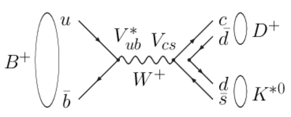
Feynman diagrams for $ B^{+} \rightarrow D_s^{+}\phi$ , $ B ^+ \rightarrow D ^+ K ^{*0} $ and $ B ^+ \rightarrow D ^+_ s \overline{ K }{} ^{*0} $ decays. |
b2dsph[..].pdf [7 KiB] HiDef png [53 KiB] Thumbnail [102 KiB] *.C file |

|
|
b2dkst[..].pdf [7 KiB] HiDef png [56 KiB] Thumbnail [89 KiB] *.C file |
|
|
|
b2dsks[..].pdf [7 KiB] HiDef png [57 KiB] Thumbnail [89 KiB] *.C file |

|
|
|
Fit results for $ B^{+} \rightarrow D_s^{+}\phi$ . The fit regions, as given in Table 1, are labelled on the panels. The PDF components are as given in the legend. |
B2Dsphi.pdf [27 KiB] HiDef png [381 KiB] Thumbnail [297 KiB] *.C file |

|
|
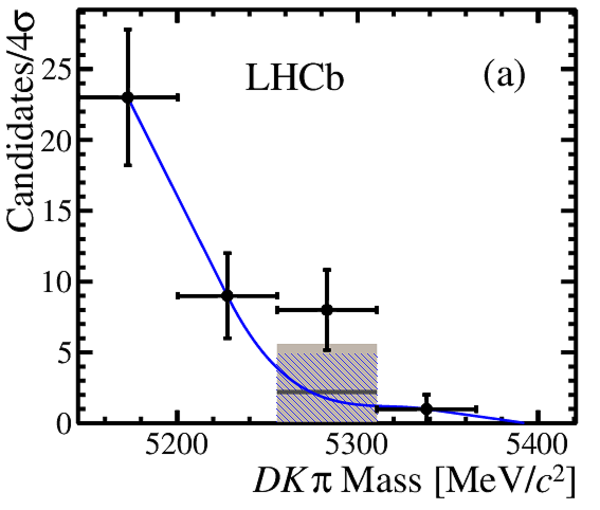
Invariant mass distributions for (a) $ B ^+ \rightarrow D ^+ K ^{*0} $ , (b) $ B ^+ \rightarrow D ^+ \overline{ K }{} ^{*0} $ , (c) ${ B ^+ \rightarrow D ^+_ s K ^{*0} }$ and (d) $ B ^+ \rightarrow D ^+_ s \overline{ K }{} ^{*0} $ . The bins are each $4\sigma$ wide, where ${\sigma =13.8}$ $ {\mathrm{ Me V /}c^2}$ is the expected width of the signal peaks (the middle bin is centred at the expected $B^+$ mass). The shaded regions are the $\mu_{\rm bkgd}\pm\sigma_{\rm bkgd}$ intervals (see Table 3) used for the limit calculations; they are taken from the truncated-Gaussian priors as discussed in the text. Spline interpolation results (solid blue line and hashed blue areas) are shown for comparison. |
dkstar[..].pdf [14 KiB] HiDef png [229 KiB] Thumbnail [191 KiB] *.C file |
|
|
dkstar[..].pdf [14 KiB] HiDef png [273 KiB] Thumbnail [216 KiB] *.C file |

|
|
|
dsksta[..].pdf [14 KiB] HiDef png [256 KiB] Thumbnail [204 KiB] *.C file |

|
|
|
dsksta[..].pdf [14 KiB] HiDef png [227 KiB] Thumbnail [187 KiB] *.C file |

|
|
|
Animated gif made out of all figures. |
PAPER-2012-025.gif Thumbnail |

|
![HiDef png [53 KiB]](Directory_LHCb-PAPER-2012-025/hidef_b2dsphi_feyn.png)
![HiDef png [56 KiB]](Directory_LHCb-PAPER-2012-025/hidef_b2dkstar_feyn.png)
![HiDef png [57 KiB]](Directory_LHCb-PAPER-2012-025/hidef_b2dskstar_feyn.png)
![HiDef png [381 KiB]](Directory_LHCb-PAPER-2012-025/hidef_B2Dsphi.png)
![HiDef png [229 KiB]](Directory_LHCb-PAPER-2012-025/hidef_dkstar_ss_final.png)
![HiDef png [273 KiB]](Directory_LHCb-PAPER-2012-025/hidef_dkstar_os_final.png)
![HiDef png [256 KiB]](Directory_LHCb-PAPER-2012-025/hidef_dskstar_ss_final.png)
![HiDef png [227 KiB]](Directory_LHCb-PAPER-2012-025/hidef_dskstar_os_final.png)
Tables and captions
|
Summary of fit regions for $ B ^+ \rightarrow D ^+_ s \phi$. About 89% of the signal is expected to be in region A. |
Table_1.pdf [42 KiB] HiDef png [43 KiB] Thumbnail [19 KiB] tex code |

|
|
Systematic uncertainties contributing to $\mathcal{B}( B^{+} \rightarrow D_s^{+}\phi )/\mathcal{B}( B ^+ \rightarrow D ^+_ s \overline{ D }{} ^0 )$. |
Table_2.pdf [16 KiB] HiDef png [58 KiB] Thumbnail [25 KiB] tex code |

|
|
Upper limits on $\cal B (B^\pm \rightarrow D_{(s)}^{\pm} K ^{*0} )$, where $n_{\rm obs}$ is the number of events observed in each of the signal regions, while $\mu_{\rm bkgd}$ and $\sigma_{\rm bkgd}$ are the Gaussian parameters used in the background prior PDFs. |
Table_3.pdf [53 KiB] HiDef png [43 KiB] Thumbnail [21 KiB] tex code |

|
|
Upper limits on $f_c/f_u \cdot \mathcal{B}(B_c \rightarrow X)$, where $n_{\rm obs}$ and $n_{\rm bkgd}$ are the number of events observed in the signal and background (sideband) regions, respectively. |
Table_4.pdf [53 KiB] HiDef png [52 KiB] Thumbnail [26 KiB] tex code |

|
![HiDef png [43 KiB]](Directory_LHCb-PAPER-2012-025/hidef_Table_1.png)
![HiDef png [58 KiB]](Directory_LHCb-PAPER-2012-025/hidef_Table_2.png)
![HiDef png [43 KiB]](Directory_LHCb-PAPER-2012-025/hidef_Table_3.png)
![HiDef png [52 KiB]](Directory_LHCb-PAPER-2012-025/hidef_Table_4.png)
Created on 03 May 2024.