A model-independent Dalitz plot analysis of $B^\pm \to D K^\pm$ with $D \to K^0_{\rm S} h^+h^-$ ($h=\pi, K$) decays and constraints on the CKM angle $\gamma$

Information

LHCb-PAPER-2012-027
CERN-PH-EP-2012-268
arXiv:1209.5869 [PDF]

(Submitted on 26 Sep 2012)
Phys. Lett. B718 (2012) 43
Inspire 1188164

Tools

Abstract

A binned Dalitz plot analysis of $B^\pm \to D K^\pm$ decays, with $D \to K^0_{\rm S} \pi^+\pi^-$ and $D \to K^0_{\rm S} K^+ K^-$, is performed to measure the CP-violating observables $x_{\pm}$ and $y_{\pm}$ which are sensitive to the CKM angle $\gamma$. The analysis exploits 1.0 $\rm fb^{-1}$ of data collected by the LHCb experiment. The study makes no model-based assumption on the variation of the strong phase of the D decay amplitude over the Dalitz plot, but uses measurements of this quantity from CLEO-c as input. The values of the parameters are found to be $x_- = (0.0 \pm 4.3 \pm 1.5 \pm 0.6) \times 10^{-2}$, $y_- = (2.7 \pm 5.2 \pm 0.8 \pm 2.3) \times 10^{-2}$, $x_+ = (-10.3 \pm 4.5 \pm 1.8 \pm 1.4)\times 10^{-2}$ and $y_+ = (-0.9 \pm 3.7 \pm 0.8 \pm 3.0)\times 10^{-2}$. The first, second, and third uncertainties are the statistical, the experimental systematic, and the error associated with the precision of the strong-phase parameters measured at CLEO-c, respectively. These results correspond to $\gamma = (44^{ +43}_{ -38})^\circ$, with a second solution at $\gamma \to \gamma + 180^\circ$, and $r_B = 0.07 \pm 0.04$, where $r_B$ is the ratio between the suppressed and favoured B decay amplitudes.

Figures and captions

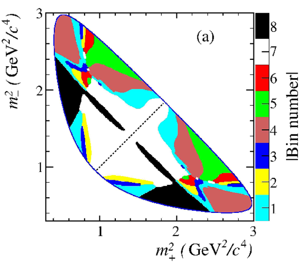
Binning choices for (a) $D \rightarrow K ^0_{\rm\scriptscriptstyle S} \pi^+\pi^-$ and (b) $D \rightarrow K ^0_{\rm\scriptscriptstyle S} K^+K^-$. The diagonal line separates the positive and negative bins.	dkpp_b[..].pdf [211 KiB] HiDef png [938 KiB] Thumbnail [292 KiB] *.C file
	dkpp_k[..].pdf [198 KiB] HiDef png [645 KiB] Thumbnail [211 KiB] *.C file
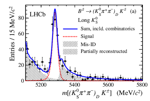
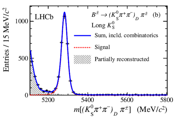
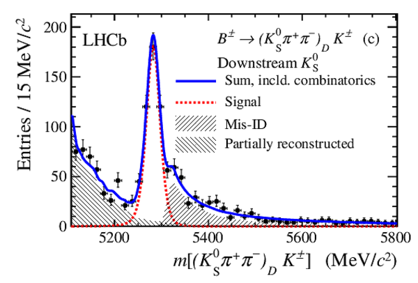
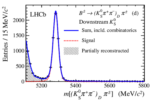
Invariant mass distributions of (a,c) $B^\pm \rightarrow D K^\pm$ and (b,d) $B^\pm \rightarrow D \pi^\pm$ candidates, with $D \rightarrow K ^0_{\rm\scriptscriptstyle S} \pi^+\pi^-$, divided between the (a,b) long and (c,d) downstream $ K ^0_{\rm\scriptscriptstyle S}$ categories. Fit results, including the signal and background components, are superimposed.	d2kspi[..].pdf [11 KiB] HiDef png [315 KiB] Thumbnail [262 KiB] *.C file
	d2kspi[..].pdf [9 KiB] HiDef png [240 KiB] Thumbnail [200 KiB] *.C file
	d2kspi[..].pdf [11 KiB] HiDef png [315 KiB] Thumbnail [263 KiB] *.C file
	d2kspi[..].pdf [9 KiB] HiDef png [257 KiB] Thumbnail [218 KiB] *.C file
Invariant mass distributions of (a) $B^\pm \rightarrow D K^\pm$ and (b) $B^\pm \rightarrow D \pi^\pm$ candidates, with $D \rightarrow K ^0_{\rm\scriptscriptstyle S} K^+K^-$, shown with both $ K ^0_{\rm\scriptscriptstyle S}$ categories combined. Fit results, including the signal and background components, are superimposed.	d2kskk[..].pdf [11 KiB] HiDef png [291 KiB] Thumbnail [245 KiB] *.C file
	d2kskk[..].pdf [9 KiB] HiDef png [241 KiB] Thumbnail [200 KiB] *.C file
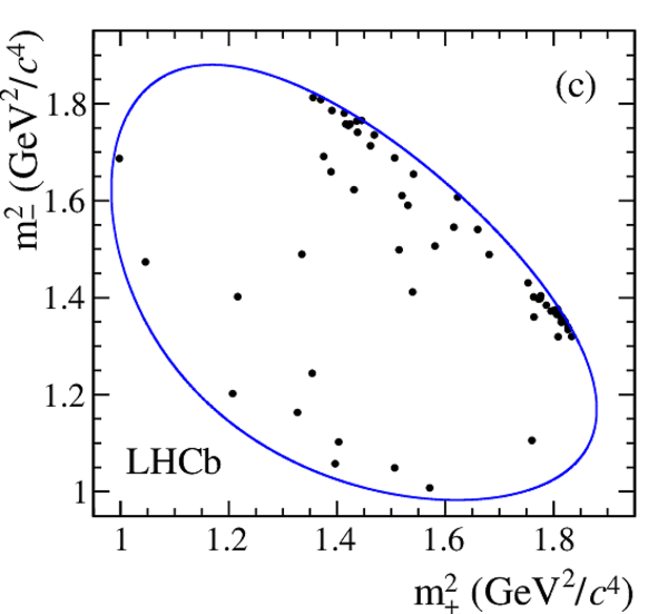
Dalitz plots of $B^\pm \rightarrow D K^\pm$ candidates in the signal region for (a,b) $D \rightarrow K ^0_{\rm\scriptscriptstyle S} \pi^+\pi^-$ and (c,d) $D \rightarrow K ^0_{\rm\scriptscriptstyle S} K^+ K^-$ decays, divided between (a,c) $B^+$ and (b,d) $B^-$. The boundaries of the kinematically-allowed regions are also shown.	Dalitz[..].pdf [34 KiB] HiDef png [199 KiB] Thumbnail [178 KiB] *.C file
	Dalitz[..].pdf [34 KiB] HiDef png [210 KiB] Thumbnail [189 KiB] *.C file
	Dalitz[..].pdf [17 KiB] HiDef png [171 KiB] Thumbnail [142 KiB] *.C file
	Dalitz[..].pdf [17 KiB] HiDef png [173 KiB] Thumbnail [145 KiB] *.C file
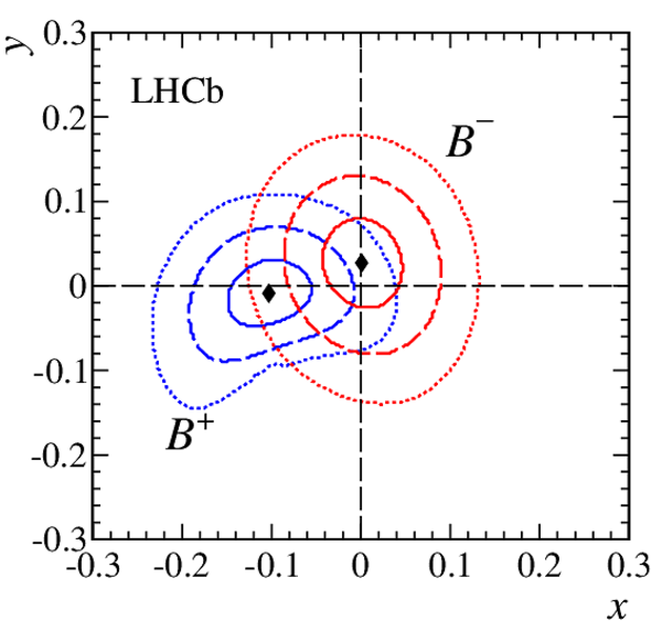
One (solid), two (dashed) and three (dotted) standard deviation confidence levels for $(x_+,y_+)$ (blue) and $(x_{-}, y_{-})$ (red) as measured in $B^\pm \rightarrow D K^\pm$ decays (statistical only). The points represent the best fit central values.	likescan.pdf [8 KiB] HiDef png [211 KiB] Thumbnail [174 KiB] *.C file
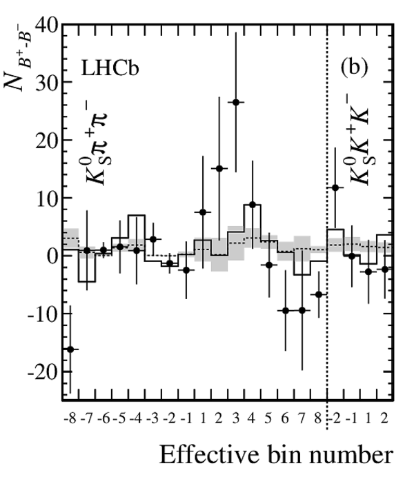
Signal yield in effective bins compared with prediction of $(x_\pm, y_\pm)$ fit (black histogram) for $D \rightarrow K ^0_{\rm\scriptscriptstyle S} \pi^+\pi^-$ and $D \rightarrow K ^0_{\rm\scriptscriptstyle S} K^+K^-$. Figure (a) shows the sum of $B^+$ and $B^-$ yields. Figure (b) shows the difference of $B^+$ and $B^-$ yields. Also shown (dashed line and grey shading) is the expectation and uncertainty for the zero $ C P$ -violation hypothesis.	BplusB[..].pdf [6 KiB] HiDef png [155 KiB] Thumbnail [89 KiB] *.C file
	BplusB[..].pdf [15 KiB] HiDef png [166 KiB] Thumbnail [101 KiB] *.C file
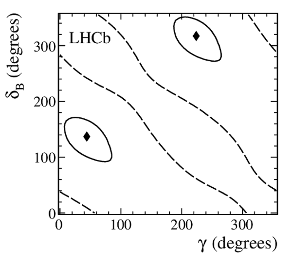
Two-dimensional projections of confidence regions onto the $(\gamma, r_B)$ and $(\gamma, \delta_B)$ planes showing the one (solid) and two (dashed) standard deviations with all uncertainties included. For the ($\gamma,r_B$) projection the three (dotted) standard deviation contour is also shown. The points mark the central values.	fr_con[..].pdf [4 KiB] HiDef png [123 KiB] Thumbnail [68 KiB] *.C file
	fd_con[..].pdf [5 KiB] HiDef png [125 KiB] Thumbnail [69 KiB] *.C file
Animated gif made out of all figures.	PAPER-2012-027.gif Thumbnail

Tables and captions

Yields and statistical uncertainties in the signal region from the invariant mass fit, scaled from the full fit mass range, for candidates passing the $B^\pm \rightarrow D h^\pm$, $D \rightarrow K ^0_{\rm\scriptscriptstyle S} \pi^+\pi^-$ selection. Values are shown separately for candidates containing long and downstream $ K ^0_{\rm\scriptscriptstyle S}$ decays. The signal region is between 5247 $ {\mathrm{ Me V /}c^2}$ and 5317 $ {\mathrm{ Me V /}c^2}$ and the full fit range is between 5110 $ {\mathrm{ Me V /}c^2}$ and 5800 $ {\mathrm{ Me V /}c^2}$ .	Table_1.pdf [39 KiB] HiDef png [48 KiB] Thumbnail [23 KiB] tex code
Yields and statistical uncertainties in the signal region from the invariant mass fit, scaled from the full fit mass range, for candidates passing the $B^\pm \rightarrow D h^\pm$, $D \rightarrow K ^0_{\rm\scriptscriptstyle S} K^+K^-$ selection. Values are shown separately for candidates containing long and downstream $ K ^0_{\rm\scriptscriptstyle S}$ decays. The signal region is between 5247 $ {\mathrm{ Me V /}c^2}$ and 5317 $ {\mathrm{ Me V /}c^2}$ and the full fit range is between 5110 $ {\mathrm{ Me V /}c^2}$ and 5800 $ {\mathrm{ Me V /}c^2}$ .	Table_2.pdf [39 KiB] HiDef png [49 KiB] Thumbnail [23 KiB] tex code
Results for $x_{\pm}$ and $y_{\pm}$ from the fits to the data in the case when both $D \rightarrow K ^0_{\rm\scriptscriptstyle S} \pi^+\pi^-$ and $D \rightarrow K ^0_{\rm\scriptscriptstyle S} K^+K^-$ are considered and when only the $D \rightarrow K ^0_{\rm\scriptscriptstyle S} \pi^+\pi^-$ final state is included. The first, second, and third uncertainties are the statistical, the experimental systematic, and the error associated with the precision of the strong-phase parameters, respectively. The correlation coefficients are calculated including all sources of uncertainty (the values in parentheses correspond to the case where only the statistical uncertainties are considered).	Table_3.pdf [52 KiB] HiDef png [68 KiB] Thumbnail [38 KiB] tex code
Summary of statistical, experimental and strong-phase uncertainties on $x_\pm$ and $y_\pm$ in the case where both $D \rightarrow K ^0_{\rm\scriptscriptstyle S} \pi^+\pi^-$ and $D \rightarrow K ^0_{\rm\scriptscriptstyle S} K^+K^-$ decays are included in the fit. All entries are given in multiples of $10^{-2}$.	Table_4.pdf [50 KiB] HiDef png [103 KiB] Thumbnail [47 KiB] tex code
Summary of statistical, experimental and strong-phase uncertainties on $x_\pm$ and $y_\pm$ in the case where only $D \rightarrow K ^0_{\rm\scriptscriptstyle S} \pi^+\pi^-$ decays are included in the fit. All entries are given in multiples of $10^{-2}$.	Table_5.pdf [50 KiB] HiDef png [103 KiB] Thumbnail [47 KiB] tex code