Analysis of the resonant components in $\overline{B}^0 \to J/\psi \pi^+ \pi^-$

Information

LHCb-PAPER-2012-045
CERN-PH-EP-2013-004
arXiv:1301.5347 [PDF]

(Submitted on 22 Jan 2013)
Phys. Rev. D87 (2013) 052001
Inspire 1215769

Tools

Abstract

Interpretation of CP violation measurements using charmonium decays, in both the B0 and Bs systems, can be subject to changes due to "penguin" type diagrams. These effects can be investigated using measurements of the Cabibbo-suppressed B0->J/\psi pi+pi- decays. The final state composition of this channel is investigated using a 1.0/fb sample of data produced in 7 TeV pp collisions at the LHC and collected by the LHCb experiment. A modified Dalitz plot analysis is performed using both the invariant mass spectra and the decay angular distributions. An improved measurement of the B0->J/\psi pi+pi- branching fraction of (3.97 +/-0.09+/- 0.11 +/- 0.16)x10^{-5} is reported where the first uncertainty is statistical, the second is systematic and the third is due to the uncertainty of the branching fraction of the decay B- -> J/\psi K- used as a normalization channel. In the J/\psi pi+pi- final state significant production of f0(500) and rho(770) resonances is found, both of which can be used for CP violation studies. In contrast evidence for the f0(980) resonance is not found, thus establishing the first upper limit on the branching fraction product B(B0->J/\psi f0(980) x B(f0(980)-> pi+ pi-) < 1.1x10^{-6}, leading to an upper limit on the absolute value of the mixing angle of the f0(980)$ with the f0(500) of <31 degrees, both at 90% confidence level.

Figures and captions

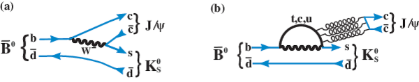
(a) Tree level and (b) penguin diagram examples for $\overline{ B }{} ^0 $ decays into $ { J \mskip -3mu/\mskip -2mu\psi \mskip 2mu} K ^0_{\rm\scriptscriptstyle S} $.	feyn4.pdf [56 KiB] HiDef png [90 KiB] Thumbnail [85 KiB] *.C file
(a) Tree level and (b) penguin diagram for $\overline{ B }{} ^0 $ decays into $ { J \mskip -3mu/\mskip -2mu\psi \mskip 2mu} \pi^+\pi^-$.	feyn3.pdf [58 KiB] HiDef png [101 KiB] Thumbnail [95 KiB] *.C file
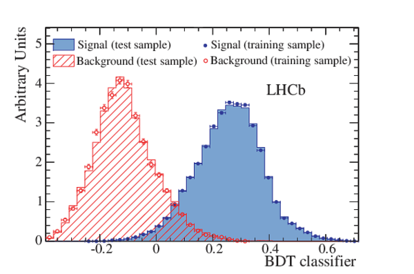
Distributions of the BDT classifier for both training and test samples of $ { J \mskip -3mu/\mskip -2mu\psi \mskip 2mu} \pi^+\pi^-$ signal and background events. The signal samples are from simulation and the background samples are from data.	overtr[..].pdf [33 KiB] HiDef png [293 KiB] Thumbnail [240 KiB] *.C file
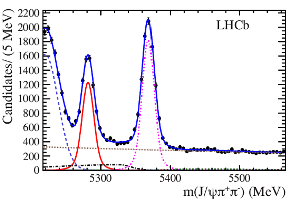
Invariant mass of $ { J \mskip -3mu/\mskip -2mu\psi \mskip 2mu} \pi^+\pi^-$ combinations. The data are fitted with a double-Gaussian signal and several background functions. The (red) solid double-Gaussian function centered at 5280 $\mathrm{ Me V}$ is the $\overline{ B }{} ^0 $ signal, the (brown) dotted line shows the combinatorial background, the (green) short-dashed shows the $B^-$ background, the (purple) dot-dashed line shows the contribution of $\overline{ B }{} ^0_ s \rightarrow { J \mskip -3mu/\mskip -2mu\psi \mskip 2mu} \pi^+\pi^-$ decays, the (black) dot-long dashed is the sum of $\overline{ B }{} ^0_ s \rightarrow { J \mskip -3mu/\mskip -2mu\psi \mskip 2mu} \eta'(\rightarrow \rho \gamma)$ and $\overline{ B }{} ^0_ s \rightarrow { J \mskip -3mu/\mskip -2mu\psi \mskip 2mu} \phi(\rightarrow \pi^+\pi^-\pi^0)$ backgrounds, the (light blue) long-dashed is the $\overline{ B }{} ^0 \rightarrow { J \mskip -3mu/\mskip -2mu\psi \mskip 2mu} K^- \pi^+$ reflection, and the (blue) solid line is the total.	fitmas[..].pdf [44 KiB] HiDef png [430 KiB] Thumbnail [227 KiB] *.C file
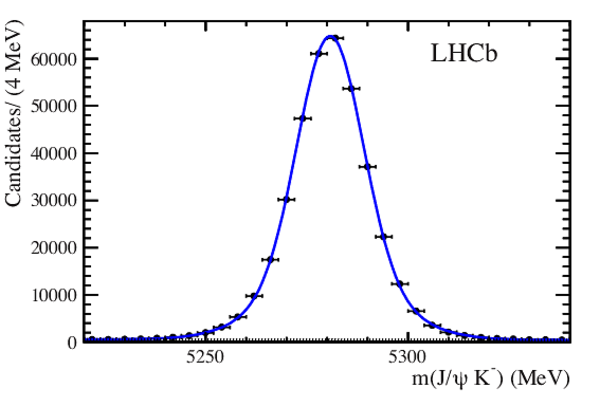
Invariant mass of $ { J \mskip -3mu/\mskip -2mu\psi \mskip 2mu} K^-$ combinations. The data points are fitted with a double-Gaussian function for signal and a linear function for background. The dotted line shows the background, and the (blue) solid line is the total.	Bu2JpsiK.pdf [34 KiB] HiDef png [231 KiB] Thumbnail [131 KiB] *.C file
Distribution of $m^2(\pi^+\pi^-)$ versus $m^2( { J \mskip -3mu/\mskip -2mu\psi \mskip 2mu} \pi^+)$ for $\overline{ B }{} ^0 $ candidate decays within $\pm20$ $\mathrm{ Me V}$ of the $\overline{ B }{} ^0 $ mass.	dalitz.pdf [130 KiB] HiDef png [486 KiB] Thumbnail [500 KiB] *.C file
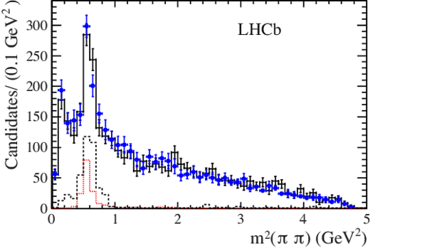
Distribution of (a) $m( { J \mskip -3mu/\mskip -2mu\psi \mskip 2mu} \pi^+)$ and (b) $m(\pi^+\pi^-)$ for $\overline{ B }{} ^0 \rightarrow { J \mskip -3mu/\mskip -2mu\psi \mskip 2mu} \pi^+\pi^-$ candidate decays within $\pm20$ $\mathrm{ Me V}$ of $\overline{ B }{} ^0 $ mass shown with the solid line. The (red) points with error bars show the background contribution determined from $m( { J \mskip -3mu/\mskip -2mu\psi \mskip 2mu} \pi^+\pi^-)$ fits performed in each bin.	m-jpsipi.pdf [39 KiB] HiDef png [233 KiB] Thumbnail [145 KiB] *.C file
	m-pipi.pdf [39 KiB] HiDef png [257 KiB] Thumbnail [159 KiB] *.C file
Distributions of $\cos\theta_{ { J \mskip -3mu/\mskip -2mu\psi \mskip 2mu} }$ for the $ { J \mskip -3mu/\mskip -2mu\psi \mskip 2mu} \pi^+\pi^-$ simulated sample in (a) the entire dipion mass region and (b) $\rho(770)$ region.	cosH_eff.pdf [35 KiB] HiDef png [235 KiB] Thumbnail [136 KiB] *.C file
	cosH_e[..].pdf [36 KiB] HiDef png [254 KiB] Thumbnail [157 KiB] *.C file
Exponential fit to the acceptance parameter $a(s_{12})$ used in Eq. 18.	cosHacc.pdf [11 KiB] HiDef png [129 KiB] Thumbnail [126 KiB] *.C file
Parametrized detection efficiency as a function of $m^2(\pi^+\pi^-)$ versus $m^2( { J \mskip -3mu/\mskip -2mu\psi \mskip 2mu} \pi^+)$ determined from simulation. The $z$-axis scale is arbitrary.	effmodel.pdf [519 KiB] HiDef png [1 MiB] Thumbnail [439 KiB] *.C file
Projections onto (a) $m^2( { J \mskip -3mu/\mskip -2mu\psi \mskip 2mu} \pi^+)$ and (b) $m^2(\pi^+\pi^-)$ of the simulated Dalitz plot used to determine the efficiency parameters. The points represent the simulated event distributions and the curves the projections of the polynomial fits.	effx.pdf [38 KiB] HiDef png [184 KiB] Thumbnail [144 KiB] *.C file
	effy.pdf [38 KiB] HiDef png [189 KiB] Thumbnail [154 KiB] *.C file
The $m^2(\pi\pi)$ distribution of background. The (black) histogram with error bars shows the same-sign data combinations with additional background from simulation, the (blue) points with error bars show the background obtained from the mass fits, the (black) dashed line is the partially reconstructed $\overline{ B }{} ^0_ s $ background, and the (red) dotted is the misidentified $\overline{ B }{} ^0 \rightarrow { J \mskip -3mu/\mskip -2mu\psi \mskip 2mu} K^- \pi^+$ contribution.	bkgcmp.pdf [37 KiB] HiDef png [199 KiB] Thumbnail [155 KiB] *.C file
Projections of invariant mass squared of (a) $m^2( { J \mskip -3mu/\mskip -2mu\psi \mskip 2mu} \pi^+)$ and (b) $m^2(\pi^+\pi^-)$ of the background Dalitz plot. The points with error bars show the same-sign combinations with additional background from simulation.	x_bkgnew.pdf [39 KiB] HiDef png [194 KiB] Thumbnail [181 KiB] *.C file
	y_bkgnew.pdf [38 KiB] HiDef png [186 KiB] Thumbnail [163 KiB] *.C file
distribution of the background in $\cos\theta_{ { J \mskip -3mu/\mskip -2mu\psi \mskip 2mu} }$ resulting from $ { J \mskip -3mu/\mskip -2mu\psi \mskip 2mu} \pi^+\pi^-$ candidate mass fits in each bin of $\cos\theta_{ { J \mskip -3mu/\mskip -2mu\psi \mskip 2mu} }$. The curve represents the fitted function $1+\alpha\cos^2\theta_{ { J \mskip -3mu/\mskip -2mu\psi \mskip 2mu} }$.	bkg_cosH.pdf [35 KiB] HiDef png [208 KiB] Thumbnail [135 KiB] *.C file
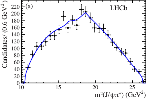
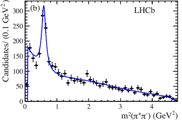
Dalitz fit projections of (a) $m^2(\pi^+\pi^-)$, (b) $m^2( { J \mskip -3mu/\mskip -2mu\psi \mskip 2mu} \pi^{+})$, (c) $\cos \theta_{ { J \mskip -3mu/\mskip -2mu\psi \mskip 2mu} }$ and (d) $m(\pi^+\pi^-)$ for the best model. The points with error bars are data, the signal fit is shown with a (red) dashed line, the background with a (black) dotted line, and the (blue) solid line represents the total. In (a) and (d), the shape variations near the $\rho(770)$ mass is due to $\rho(770)-\omega(782)$ interference, and the dip at the $ K ^0_{\rm\scriptscriptstyle S} $ mass [31] is due to the $ K ^0_{\rm\scriptscriptstyle S} $ veto.	y.pdf [40 KiB] HiDef png [225 KiB] Thumbnail [176 KiB] *.C file
	x.pdf [40 KiB] HiDef png [208 KiB] Thumbnail [185 KiB] *.C file
	cosH.pdf [37 KiB] HiDef png [239 KiB] Thumbnail [165 KiB] *.C file
	mpp.pdf [39 KiB] HiDef png [283 KiB] Thumbnail [172 KiB] *.C file
Helicity angle distributions of (a) $\cos \theta_{ { J \mskip -3mu/\mskip -2mu\psi \mskip 2mu} }$ ($\chi^2$/ndf =15/20) and (b) $\cos\theta_{\pi\pi}$ ($\chi^2$/ndf =14/20) in the $\rho(770)$ mass region defined within one full width of the $\rho(770)$ mass. The points with error bars are data, the signal fit to the best model is shown with a (red) dashed line, the background with a (black) dotted line, and the (blue) solid line represents the total.	cosH_rho.pdf [35 KiB] HiDef png [217 KiB] Thumbnail [142 KiB] *.C file
	cospp_rho.pdf [36 KiB] HiDef png [227 KiB] Thumbnail [149 KiB] *.C file
Background subtracted and efficiency corrected helicity distributions of (a) $\cos \theta_{ { J \mskip -3mu/\mskip -2mu\psi \mskip 2mu} }$ ($\chi^2$/ndf =20/20) and (b) $\cos\theta_{\pi\pi}$ ($\chi^2$/ndf =13/20) in the $\rho(770)$ mass region defined within one full width of the $\rho(770)$ mass. The points with error bars are data and the solid blue lines show the fit to the best model.	cosH_r[..].pdf [35 KiB] HiDef png [267 KiB] Thumbnail [161 KiB] *.C file
	cospp_[..].pdf [35 KiB] HiDef png [270 KiB] Thumbnail [158 KiB] *.C file
Animated gif made out of all figures.	PAPER-2012-045.gif Thumbnail

Tables and captions

Efficiency parameters to describe the acceptance on the signal Dalitz-plot.	Table_1.pdf [44 KiB] HiDef png [115 KiB] Thumbnail [50 KiB] tex code
Parameters for the background model used in Eq. 23.	Table_2.pdf [45 KiB] HiDef png [131 KiB] Thumbnail [63 KiB] tex code
Possible resonances in the $\overline{ B }{} ^0 \rightarrow { J \mskip -3mu/\mskip -2mu\psi \mskip 2mu} \pi^+\pi^-$ decay mode.	Table_3.pdf [38 KiB] HiDef png [124 KiB] Thumbnail [56 KiB] tex code
Breit-Wigner resonance parameters.	Table_4.pdf [54 KiB] HiDef png [106 KiB] Thumbnail [55 KiB] tex code
Values of $\chi^2/\text{ndf}$ and $\rm -ln\mathcal{L}$ of different resonance models.	Table_5.pdf [39 KiB] HiDef png [82 KiB] Thumbnail [39 KiB] tex code
Fit fractions and significances of contributing components for the best model, as well as the fractions of the helicity $\lambda=0$ part. The significance takes into account both statistical and systematic uncertainties.	Table_6.pdf [54 KiB] HiDef png [73 KiB] Thumbnail [35 KiB] tex code
Interference fractions ${\cal{F}}_{\lambda}^{RR'}$ (%) computed using Eq 25. Note that the diagonal elements are fit fractions defined in Eq 24.	Table_7.pdf [35 KiB] HiDef png [56 KiB] Thumbnail [25 KiB] tex code
Resonant phases from the best fit.	Table_8.pdf [38 KiB] HiDef png [187 KiB] Thumbnail [82 KiB] tex code
Fit fractions (%) of contributing components for the best model with adding one additional resonance.	Table_9.pdf [52 KiB] HiDef png [97 KiB] Thumbnail [48 KiB] tex code
Branching fractions for each channel. The upper limit at 90% CL is also quoted for the $f_0(980)$ resonance which has a significance smaller than 3$\sigma$. The first uncertainty is statistical and the second the total systematic.	Table_10.pdf [55 KiB] HiDef png [77 KiB] Thumbnail [39 KiB] tex code
Relative systematic uncertainties on branching fractions (%).	Table_11.pdf [49 KiB] HiDef png [104 KiB] Thumbnail [48 KiB] tex code
Absolute systematic uncertainties on the results of the Dalitz analysis.	Table_12.pdf [56 KiB] HiDef png [101 KiB] Thumbnail [47 KiB] tex code
Masses of light vector and scalar resonances. All values are taken from [31], except for the $f_0(500)$ [43].	Table_13.pdf [38 KiB] HiDef png [28 KiB] Thumbnail [11 KiB] tex code