Measurement of $CP$ violation and the $B_s^0$ meson decay width difference with $B_s^0 \to J/\psi K^+K^-$ and $B_s^0\to J/\psi\pi^+\pi^-$ decays

Information

LHCb-PAPER-2013-002
CERN-PH-EP-2013-055
arXiv:1304.2600 [PDF]

(Submitted on 09 Apr 2013)
Phys. Rev. D87 (2013) 112010
Inspire 1227656

Tools

Abstract

The time-dependent CP asymmetry in B_s^0\to J/\psi K^+K^- decays is measured using $pp$ collision data at \sqrt{s}=7TeV, corresponding to an integrated luminosity of 1.0fb^-1, collected with the LHCb detector. The decay time distribution is characterised by the decay widths \Gamma_L and \Gamma_H of the light and heavy mass eigenstates of the B_s^0--\bar{B}_s^0 system and by a CP-violating phase \phi_s. In a sample of 27 617 B_s^0\to J/\psi K^+K^- decays, where the dominant contribution comes from B_s^0\to J/\psi\phi decays, these parameters are measured to be \phi_s = 0.07 \pm 0.09 (stat) \pm 0.01 (syst) rad, \Gamma_s \equiv (\Gamma_L+\Gamma_H)/2 = 0.663 \pm 0.005 (stat) \pm 0.006 (syst) ps^-1, \Delta\Gamma_s \equiv \Gamma_L -\Gamma_H = 0.100 \pm 0.016 (stat) \pm 0.003 (syst) & ps^-1, corresponding to the single most precise determination of \phi_s, \Delta\Gamma_s and \Gamma_s. The result of performing a combined analysis with B_s^{0} \to J/\psi \pi^+\pi^- decays gives \phi_s = 0.01 \pm 0.07 (stat) \pm 0.01 (syst) rad, \Gamma_s = 0.661 \pm 0.004 (stat) \pm 0.006 (syst) ps^-1, \Delta\Gamma_s = 0.106 \pm 0.011 (stat) \pm 0.007 (syst) & ps^-1. All measurements are in agreement with the Standard Model predictions.

Figures and captions

Feynman diagrams for $ B ^0_ s $ -- $\overline{ B }{} ^0_ s $ mixing, within the SM.	box_di[..].pdf [40 KiB] HiDef png [28 KiB] Thumbnail [12 KiB] *.C file
Feynman diagrams contributing to the decay $ B ^0_ s \rightarrow J/\psi h^{+}h^{-}$ within the SM, where $h = \pi, K$.	tree_p[..].pdf [17 KiB] HiDef png [55 KiB] Thumbnail [23 KiB] *.C file
Definition of helicity angles as discussed in the text.	helAng[..].pdf [27 KiB] HiDef png [22 KiB] Thumbnail [10 KiB] *.C file
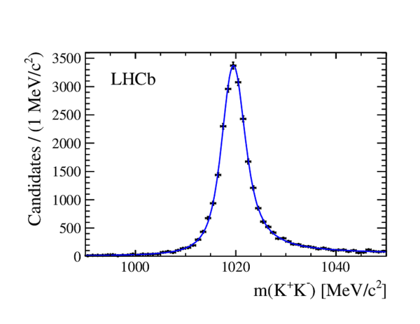
Invariant mass distribution of the selected $ B ^0_ s \rightarrow J / \psi K^{+}K^{-}$ candidates. The mass of the $\mu^{+}\mu^{-}$ pair is constrained to the $ J / \psi$ mass [8]. Curves for the fitted contributions from signal (dotted red), background (dotted green) and their combination (solid blue) are overlaid.	BMassLin.pdf [8 KiB] HiDef png [219 KiB] Thumbnail [173 KiB] *.C file
Background subtracted invariant mass distributions of the (a) $\mu^{+}\mu^{-}$ and (b) $K^{+}K^{-}$ systems in the selected sample of $ B ^0_ s \rightarrow J / \psi K^{+}K^{-}$ candidates. The solid blue line represents the fit to the data points described in the text.	mumuMa[..].pdf [9 KiB] HiDef png [164 KiB] Thumbnail [130 KiB] *.C file
	KKMassLin.pdf [9 KiB] HiDef png [158 KiB] Thumbnail [126 KiB] *.C file
Decay time resolution, $\sigma_{t}$, for selected $ B ^0_ s \rightarrow J / \psi K^{+}K^{-}$ signal events. The curve shows a fit to the data of the sum of two gamma distributions with a common mean.	Bs2Jps[..].pdf [17 KiB] HiDef png [164 KiB] Thumbnail [124 KiB] *.C file
Decay time distribution of prompt $ { J \mskip -3mu/\mskip -2mu\psi \mskip 2mu} K ^+ K ^- $ candidates. The curve (solid blue) is the decay time model convolved with a Gaussian resolution model. The decay time model consists of a delta function for the prompt component and two exponential functions with different decay constants, which represent the $ B ^0_ s \rightarrow J / \psi K^{+}K^{-}$ signal and long-lived background, respectively. The decay constants are determined from the fit. The same dataset is shown in both plots, on different scales.	presca[..].pdf [35 KiB] HiDef png [156 KiB] Thumbnail [139 KiB] *.C file
	presca[..].pdf [38 KiB] HiDef png [160 KiB] Thumbnail [150 KiB] *.C file
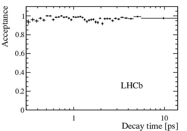
$ B ^0_ s $ decay time trigger-acceptance functions obtained from data. The unbiased trigger category is shown on (a) an absolute scale and (b) the biased trigger category on an arbitrary scale.	Bs_Hlt[..].pdf [22 KiB] HiDef png [66 KiB] Thumbnail [37 KiB] *.C file
	Bs_Hlt[..].pdf [23 KiB] HiDef png [77 KiB] Thumbnail [46 KiB] *.C file
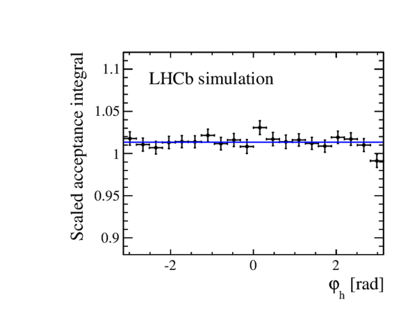
Angular acceptance function evaluated with simulated $ B ^0_ s \rightarrow J / \psi\phi$ events, scaled by the mean acceptance. The acceptance is shown as a function of (a) $\cos\theta_{K} $, (b) $\cos\theta_{\mu} $ and (c) $\varphi_{h} $, where in all cases the acceptance is integrated over the other two angles. The points are obtained by summing the inverse values of the underlying physics PDF for simulated events and the curves represent a polynomial parameterisation of the acceptance.	angEff[..].pdf [6 KiB] HiDef png [116 KiB] Thumbnail [104 KiB] *.C file
	angEff[..].pdf [6 KiB] HiDef png [130 KiB] Thumbnail [111 KiB] *.C file
	angEff[..].pdf [5 KiB] HiDef png [99 KiB] Thumbnail [96 KiB] *.C file
Average measured wrong-tag probability ($\omega$) versus estimated wrong-tag probability ($\eta$) calibrated on $ B ^+ \rightarrow { J \mskip -3mu/\mskip -2mu\psi \mskip 2mu} K ^+ $ signal events for the OS tagging combinations for the background subtracted events in the signal mass window. Points with errors are data, the red curve represents the result of the wrong-tag probability calibration, corresponding to the parameters of Table 3.	calibr[..].pdf [15 KiB] HiDef png [128 KiB] Thumbnail [111 KiB] *.C file
Distributions of the estimated wrong-tag probability, $\eta$, of the $ B ^0_ s \rightarrow J/\psi K^{+}K^{-}$ signal events obtained using the sPlot method on the $ J / \psi K^{+}K^{-}$ invariant mass distribution. Both the (a) OS-only and (b) SSK-only tagging categories are shown.	eta_OS.pdf [15 KiB] HiDef png [97 KiB] Thumbnail [59 KiB] *.C file
	eta_SSK.pdf [14 KiB] HiDef png [92 KiB] Thumbnail [54 KiB] *.C file
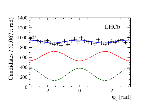
Decay-time and helicity-angle distributions for $ B ^0_ s \rightarrow { J \mskip -3mu/\mskip -2mu\psi \mskip 2mu} K ^+ K ^- $ decays (data points) with the one-dimensional projections of the PDF at the maximal likelihood point. The solid blue line shows the total signal contribution, which is composed of $ C P$ -even (long-dashed red), $ C P$ -odd (short-dashed green) and S-wave (dotted-dashed purple) contributions.	time_sFit.pdf [11 KiB] HiDef png [196 KiB] Thumbnail [148 KiB] *.C file
	helcos[..].pdf [7 KiB] HiDef png [188 KiB] Thumbnail [143 KiB] *.C file
	helcos[..].pdf [7 KiB] HiDef png [190 KiB] Thumbnail [147 KiB] *.C file
	helphi[..].pdf [8 KiB] HiDef png [177 KiB] Thumbnail [143 KiB] *.C file
Two-dimensional profile likelihood in the ($\Delta\Gamma_{ s } $, $\phi_{ s } $) plane for the $ B ^0_ s \rightarrow { J \mskip -3mu/\mskip -2mu\psi \mskip 2mu} K ^+ K ^- $ dataset. Only the statistical uncertainty is included. The SM expectation of $\Delta\Gamma_{ s } =0.087 \pm 0.021 {\rm ps^{-1}} $ and $\phi_{ s } = -0.036 \pm 0.002\rm rad $ is shown as the black point with error bar [3,43].	2DLLscan.pdf [16 KiB] HiDef png [458 KiB] Thumbnail [163 KiB] *.C file
Variation of $\delta_{\rm S}-\delta_\perp$ with $m( K ^+ K ^- )$ where the uncertainties are the quadrature sum of the statistical and systematic uncertainties in each bin. The decreasing phase trend (blue circles) corresponds to the physical solution with $\phi_{ s }$ close to zero and $\Delta\Gamma_{s}>0$. The ambiguous solution is also shown.	SWaveP[..].pdf [5 KiB] HiDef png [100 KiB] Thumbnail [83 KiB] *.C file
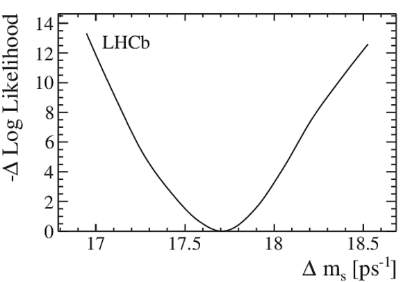
Profile likelihood for $\Delta m_{ s } $ from a fit where $\Delta m_{ s } $ is unconstrained.	LLscan[..].pdf [13 KiB] HiDef png [214 KiB] Thumbnail [118 KiB] *.C file
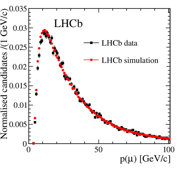
Background-subtracted (a) kaon and (b) muon momentum distributions for $B_{s}^{0}\rightarrow { J \mskip -3mu/\mskip -2mu\psi \mskip 2mu} K ^+ K ^- $ signal events in data compared to simulated $B_{s}^{0}\rightarrow { J \mskip -3mu/\mskip -2mu\psi \mskip 2mu} \phi$ signal events. The distributions are normalised to the same area. A larger deviation is visible for kaons.	pk_paper.pdf [15 KiB] HiDef png [223 KiB] Thumbnail [216 KiB] *.C file
	pmu_paper.pdf [16 KiB] HiDef png [208 KiB] Thumbnail [196 KiB] *.C file
Animated gif made out of all figures.	PAPER-2013-002.gif Thumbnail

Tables and captions

Results for $\phi_{ s } $ and $\Delta\Gamma_{s}$ from different experiments. The first uncertainty is statistical and the second is systematic (apart from the D0 result, for which the uncertainties are combined). The CDF confidence level (CL) range quoted is that consistent with other experimental measurements of $\phi_{ s }$ .	Table_1.pdf [55 KiB] HiDef png [53 KiB] Thumbnail [24 KiB] tex code
Definition of angular and time-dependent functions.	Table_2.pdf [60 KiB] HiDef png [74 KiB] Thumbnail [33 KiB] tex code
Calibration parameters ($p_0$, $p_1$,$\langle\eta\rangle$ and $\Delta p_0$) corresponding to the OS and SSK taggers. The uncertainties are statistical and systematic, respectively, except for $\Delta p_0$ where they have been added in quadrature.	Table_3.pdf [34 KiB] HiDef png [28 KiB] Thumbnail [13 KiB] tex code
Bins of $m( K ^+ K ^- )$ used in the analysis and the $C_{\rm SP}$ correction factors for the S-wave interference term, assuming a uniform distribution of non-resonant $K^{+}K^{-}$ contribution and a non-relativistic Breit-Wigner shape for the decays via the $\phi$ resonance.	Table_4.pdf [36 KiB] HiDef png [96 KiB] Thumbnail [41 KiB] tex code
Parameters of the common signal fit to the $m( J / \psi K^{+}K^{-})$ distribution in data.	Table_5.pdf [58 KiB] HiDef png [66 KiB] Thumbnail [29 KiB] tex code
Results of the maximum likelihood fit for the principal physics parameters. The first uncertainty is statistical and the second is systematic. The value of $\Delta m_{ s } $ was constrained to the measurement reported in Ref. [40]. The evaluation of the systematic uncertainties is described in Sect. 10.	Table_6.pdf [52 KiB] HiDef png [47 KiB] Thumbnail [23 KiB] tex code
Correlation matrix for the principal physics parameters.	Table_7.pdf [49 KiB] HiDef png [49 KiB] Thumbnail [24 KiB] tex code
Results of the maximum likelihood fit for the S-wave parameters, with asymmetric statistical and symmetric systematic uncertainties. The evaluation of the systematic uncertainties is described in Sect. 10.	Table_8.pdf [48 KiB] HiDef png [93 KiB] Thumbnail [48 KiB] tex code
Statistical and systematic uncertainties.	Table_9.pdf [57 KiB] HiDef png [105 KiB] Thumbnail [47 KiB] tex code
Statistical and systematic uncertainties for S-wave fractions in bins of $m(K^{+}K^{-})$.	Table_10.pdf [54 KiB] HiDef png [102 KiB] Thumbnail [45 KiB] tex code
Statistical and systematic uncertainties for S-wave phases in bins of $m(K^{+}K^{-})$.	Table_11.pdf [55 KiB] HiDef png [88 KiB] Thumbnail [36 KiB] tex code
Results of combined fit to the $B_s^0 \rightarrow J/\psi K^+K^-$ and $B_s^0 \rightarrow J/\psi \pi^+\pi^-$ datasets. The first uncertainty is statistical and the second is systematic.	Table_12.pdf [51 KiB] HiDef png [129 KiB] Thumbnail [53 KiB] tex code
Correlation matrix for statistical uncertainties on combined results.	Table_13.pdf [49 KiB] HiDef png [47 KiB] Thumbnail [24 KiB] tex code