Observation of $B^0_s$-$\bar{B}^0_s$ mixing and measurement of mixing frequencies using semileptonic B decays
[to restricted-access page]Information
LHCb-PAPER-2013-036
CERN-PH-EP-2013-143
arXiv:1308.1302 [PDF]
(Submitted on 06 Aug 2013)
Eur. Phys. J. C73 (2013) 2655
Inspire 1246784
Tools
Abstract
The $B^0_s$ and $B^0$ mixing frequencies, $\Delta m_s$ and $\Delta m_d$, are measured using a data sample corresponding to an integrated luminosity of 1.0 fb^{-1} collected by the LHCb experiment in $pp$ collisions at a centre of mass energy of 7 TeV during 2011. Around 1.8x10^6 candidate events are selected of the type $B^0_{(s)} \to D^-_{(s)} \mu^+$ (+ anything), where about half are from peaking and combinatorial backgrounds. To determine the B decay times, a correction is required for the momentum carried by missing particles, which is performed using a simulation-based statistical method. Associated production of muons or mesons allows us to tag the initial-state flavour and so to resolve oscillations due to mixing. We obtain \Delta m_s = (17.93 \pm 0.22 (stat) \pm 0.15 (syst)) ps^{-1}, \Delta m_d = (0.503 \pm 0.011 (stat) \pm 0.013 (syst)) ps^{-1}. The hypothesis of no oscillations is rejected by the equivalent of 5.8 standard deviations for $B^0_s$ and 13.0 standard deviations for $B^0$. This is the first observation of $B^0_s$ mixing to be made using only semileptonic decays.
Figures and captions
|
Mass distributions for all selected signal candidates. Left, the $K^+K^-\pi^+$ invariant mass, where the known mass of the $D^+_s$ has been subtracted. Right, the $D\mu$ normalized mass as defined in Eq. 2. Neutral candidates are those of the form $D^{\mp}\mu^\pm$, while double-charged candidates are those of the form $D^{\pm}\mu^\pm$. The double-charged candidates arise from several background sources, most of which are also present in the neutral sample. In the left plot, the neutral sample exhibits much larger $D$ mass peaks, indicative of the large $B$ signal component. |
Fig1.pdf [65 KiB] HiDef png [162 KiB] Thumbnail [142 KiB] *.C file |

|
|
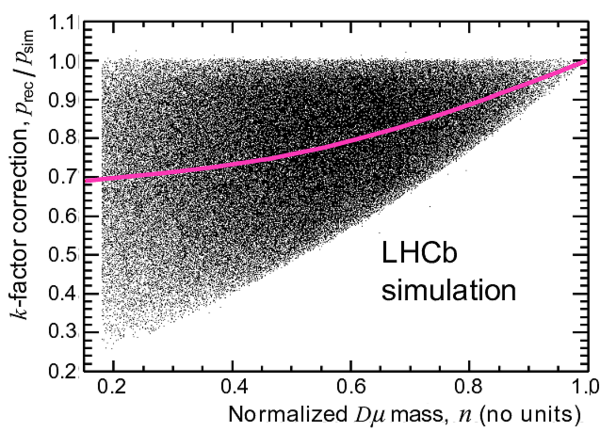
Input to obtain the $k$-factor correction from the fully-simulated $B^0_s$ sample. For each event the ratio of reconstructed to generated momentum, $p_{\textrm{rec}}/p_{\textrm{sim}}$ is plotted against the normalized $D\mu$ mass ($n$ in Eq. 2). The curve shows a fourth-order polynomial resulting from a fit to the mean of the distribution (in bins of $n$). |
Fig2.pdf [66 KiB] HiDef png [1 MiB] Thumbnail [637 KiB] *.C file |
|
|
Illustration of the decay time resolution obtained from a fully simulated $B^0$ signal sample. The left plots demonstrate the Gaussian fits (solid lines) using the full LHCb simulated data (filled), to determine the decay time resolution. Each measured (reconstructed and corrected) time, $t'$, is compared to the corresponding simulated decay time, $t$. The results are shown for several bins of $t'$. The dependence on decay time of the mean (bias, $\mu$) and width (standard deviation, $\sigma$) can be fitted with a quadratic or cubic function of either $t$ or $t'$. The right hand plot shows a quadratic fit to the widths. |
Fig3.pdf [74 KiB] HiDef png [333 KiB] Thumbnail [227 KiB] *.C file |

|
|
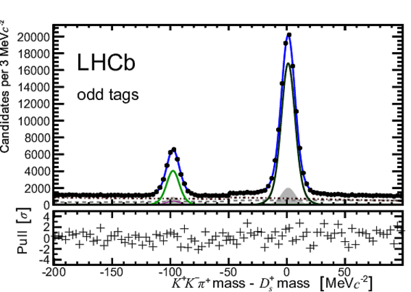
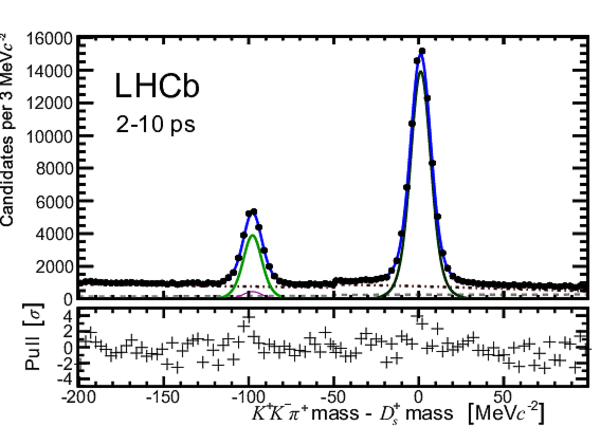
Distribution of measured $K^+K^-\pi^+$ mass, where the known mass of the $D^+_s$ has been subtracted. Black points show the data, and the various lines overlay the result of the fit. The small step at $-50$ MeV$c^{-2}$ is the result of differences in tagging efficiency for the $B^0_s$ and $B^0$ hypotheses. |
Fig4.pdf [121 KiB] HiDef png [345 KiB] Thumbnail [293 KiB] *.C file |

|
|
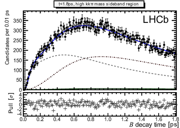
Measured $B$ decay-time distribution, overlaid with projections of the fit, for background-only regions. Top left: a region between the two signal peaks, $-80$ to $-20$ MeV$c^{-2}$ (with respect to the known mass of the $D_s^+$), showing only low decay times. Top right: a region to the right of the signal peaks $20$ to $100$ MeV$c^{-2}$, showing only low decay times. Bottom row: the same on an extended decay-time scale and logarithmic. The legend is the same as in Fig. 4. |
Fig5a-[..].pdf [100 KiB] HiDef png [370 KiB] Thumbnail [350 KiB] *.C file |

|
|
Fig5b-[..].pdf [99 KiB] HiDef png [373 KiB] Thumbnail [351 KiB] *.C file |
|
|
|
Fig5c-[..].pdf [132 KiB] HiDef png [404 KiB] Thumbnail [342 KiB] *.C file |

|
|
|
Fig5d-[..].pdf [128 KiB] HiDef png [371 KiB] Thumbnail [326 KiB] *.C file |

|
|
|
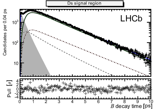
Measured $B$ decay-time distribution, overlaid with projections of the fit, for signal regions. Top left: for odd-tags, high-$n$ and a region of $\pm 20$ MeV$c^{-2}$ around the $D^+_s$ mass peak, showing only low decay times, where $B^0_s$ oscillations can be clearly seen. Top right: for odd-tags and all $n$ for a region of $\pm 20$ MeV$c^{-2}$ around the $D^+$ mass peak, showing only low decay times. Bottom row: for both tags and all $n$ for regions of $\pm 20$ MeV$c^{-2}$ around the $D^+_s$ (left) and $D^+$ (right) mass peaks. The legend is the same as in Fig. 4. |
Fig6a-[..].pdf [98 KiB] HiDef png [425 KiB] Thumbnail [376 KiB] *.C file |

|
|
Fig6b-[..].pdf [90 KiB] HiDef png [444 KiB] Thumbnail [387 KiB] *.C file |

|
|
|
Fig6c-[..].pdf [122 KiB] HiDef png [342 KiB] Thumbnail [294 KiB] *.C file |
|
|
|
Fig6d-[..].pdf [126 KiB] HiDef png [407 KiB] Thumbnail [341 KiB] *.C file |

|
|
|
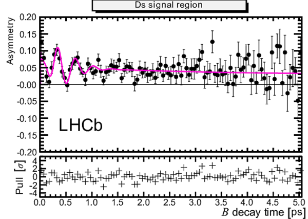
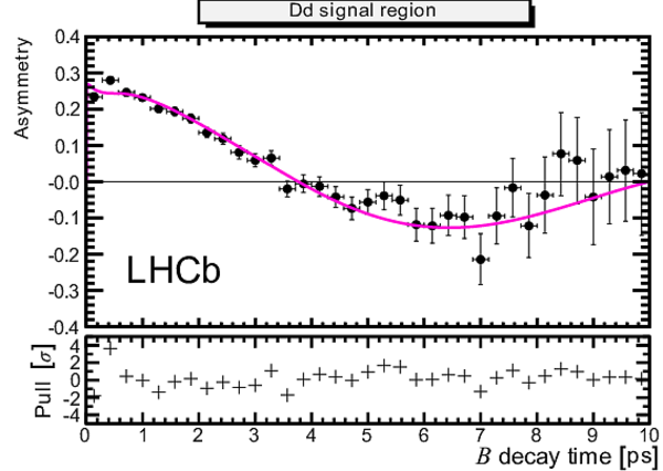
Tagged (mixing) asymmetry, $(N_+-N_-)/(N_++N_-)$, as a function of $B$ decay time. The left plot shows the asymmetry for events for a region of $\pm 20$ MeV$c^{-2}$ around the $D^+_s$ mass peak, and the right plot shows the corresponding asymmetry around the $D^+$ mass peak. The black points show the data and the curves are projections of the fitted PDF. On the left plot the fast oscillations of $B^0_s$ are gradually washed out by the increasingly poor decay-time resolution. |
Fig7a-left.pdf [77 KiB] HiDef png [299 KiB] Thumbnail [295 KiB] *.C file |
|
|
Fig7b-[..].pdf [65 KiB] HiDef png [210 KiB] Thumbnail [206 KiB] *.C file |
|
|
|
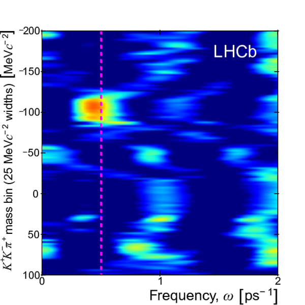
Result of using Fourier transforms to search for the $\Delta m_s$-peak. The image on the left is constructed from bins of the $K^+K^-\pi^+$ mass which are 25 MeV$c^{-2}$ in width, analysed in steps of 5 MeV$c^{-2}$ such that a smooth image is produced. The colour scale (blue-green-yellow-red) is an arbitrary linear representation of the signal intensity; dark blue is used for zero and below. The vertical dashed line is drawn at $18.0$ ps$^{-1}$. The apparent double-peak structure is an artifact of this image. On the right a slice around the $D^+_s$ mass region shows only the peak as used to measure the central value and rms width. |
Fig8a-left.pdf [214 KiB] HiDef png [2 MiB] Thumbnail [651 KiB] *.C file |

|
|
Fig8b-[..].pdf [26 KiB] HiDef png [73 KiB] Thumbnail [34 KiB] *.C file |

|
|
|
Animated gif made out of all figures. |
PAPER-2013-036.gif Thumbnail |

|
Tables and captions
|
A selection of fitted parameter values, for which statistical uncertainties only are given. The $B^0_s$ signal fraction includes contributions from any detached $D^+_s$ production. When the omitted fractions (of combinatorial background components) are included, the total fraction sums to unity within each $n$ region separately. |
Table_1.pdf [46 KiB] HiDef png [123 KiB] Thumbnail [56 KiB] tex code |

|
|
Sources of systematic uncertainty on $\Delta m_s$ and $\Delta m_d$. "Simulation" implies a combination of full LHCb simulation and pseudo-experiment studies. |
Table_2.pdf [54 KiB] HiDef png [80 KiB] Thumbnail [35 KiB] tex code |

|
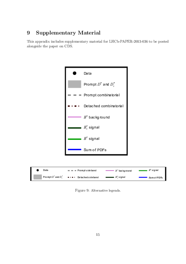
Supplementary Material [file]


![HiDef png [162 KiB]](Directory_LHCb-PAPER-2013-036/hidef_Fig1.png)
![HiDef png [1 MiB]](Directory_LHCb-PAPER-2013-036/hidef_Fig2.png)
![HiDef png [333 KiB]](Directory_LHCb-PAPER-2013-036/hidef_Fig3.png)
![HiDef png [345 KiB]](Directory_LHCb-PAPER-2013-036/hidef_Fig4.png)
![HiDef png [370 KiB]](Directory_LHCb-PAPER-2013-036/hidef_Fig5a-topleft.png)
![HiDef png [373 KiB]](Directory_LHCb-PAPER-2013-036/hidef_Fig5b-topright.png)
![HiDef png [404 KiB]](Directory_LHCb-PAPER-2013-036/hidef_Fig5c-bottomleft.png)
![HiDef png [371 KiB]](Directory_LHCb-PAPER-2013-036/hidef_Fig5d-bottomright.png)
![HiDef png [425 KiB]](Directory_LHCb-PAPER-2013-036/hidef_Fig6a-topleft.png)
![HiDef png [444 KiB]](Directory_LHCb-PAPER-2013-036/hidef_Fig6b-topright.png)
![HiDef png [342 KiB]](Directory_LHCb-PAPER-2013-036/hidef_Fig6c-bottomleft.png)
![HiDef png [407 KiB]](Directory_LHCb-PAPER-2013-036/hidef_Fig6d-bottomright.png)
![HiDef png [299 KiB]](Directory_LHCb-PAPER-2013-036/hidef_Fig7a-left.png)
![HiDef png [210 KiB]](Directory_LHCb-PAPER-2013-036/hidef_Fig7b-right.png)
![HiDef png [2 MiB]](Directory_LHCb-PAPER-2013-036/hidef_Fig8a-left.png)
![HiDef png [73 KiB]](Directory_LHCb-PAPER-2013-036/hidef_Fig8b-right.png)
![HiDef png [123 KiB]](Directory_LHCb-PAPER-2013-036/hidef_Table_1.png)
![HiDef png [80 KiB]](Directory_LHCb-PAPER-2013-036/hidef_Table_2.png)
![HiDef png [152 KiB]](Directory_LHCb-PAPER-2013-036/supplementary/hidef_CDS-Supplementary.png)
![HiDef png [299 KiB]](Directory_LHCb-PAPER-2013-036/supplementary/hidef_Fig10a-mass-odd.png)
![HiDef png [312 KiB]](Directory_LHCb-PAPER-2013-036/supplementary/hidef_Fig10b-mass-even.png)
![HiDef png [285 KiB]](Directory_LHCb-PAPER-2013-036/supplementary/hidef_Fig11a-mass-lowt.png)
![HiDef png [274 KiB]](Directory_LHCb-PAPER-2013-036/supplementary/hidef_Fig11b-mass-midt.png)
![HiDef png [276 KiB]](Directory_LHCb-PAPER-2013-036/supplementary/hidef_Fig11c-mass-hight.png)
![HiDef png [298 KiB]](Directory_LHCb-PAPER-2013-036/supplementary/hidef_Fig12-mass-log.png)
![HiDef png [3 MiB]](Directory_LHCb-PAPER-2013-036/supplementary/hidef_Fig13-Fourier-Dmd.png)
![HiDef png [37 KiB]](Directory_LHCb-PAPER-2013-036/supplementary/hidef_Fig8a-Top-Legend.png)
![HiDef png [36 KiB]](Directory_LHCb-PAPER-2013-036/supplementary/hidef_Fig8b-Bottom-Legend.png)
Created on 27 April 2024.