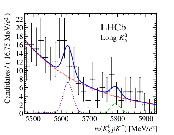
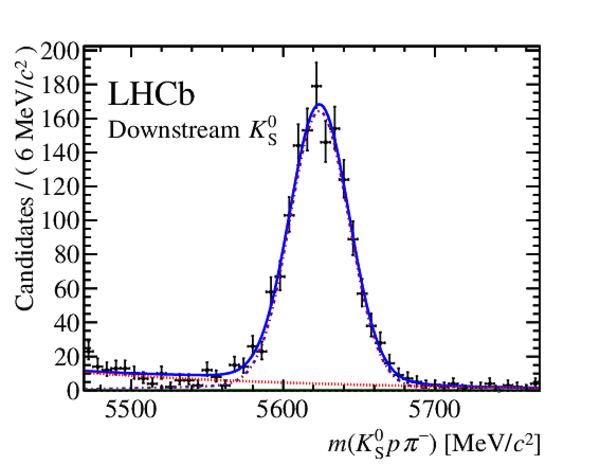
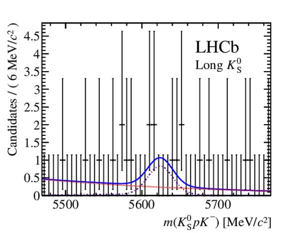
Invariant mass distribution of (top) $ K ^0_{\rm\scriptscriptstyle S} p\pi^{-}$ and (bottom) $ K ^0_{\rm\scriptscriptstyle S} pK^{-}$ candidates for the (left) Downstream and (right) Long $ K ^0_{\rm\scriptscriptstyle S}$ categories after the final selection in the full data sample. Each significant component of the fit model is displayed: $\Lambda ^0_ b $ signal (violet dot-dashed), $\Xi^{0}_{ b } $ signal (green dashed) and combinatorial background (red dotted). The overall fit is given by the solid blue line. Contributions with very small yields are not shown.

Invariant mass distribution of (top) $\Lambda ^0_ b \rightarrow \Lambda ^+_ c (\rightarrow p K ^0_{\rm\scriptscriptstyle S} ) \pi ^- $ , (middle) $\Lambda ^0_ b \rightarrow \Lambda ^+_ c (\rightarrow p K ^0_{\rm\scriptscriptstyle S} ) K ^- $ and (bottom) $\Lambda ^0_ b \rightarrow D ^-_ s (\rightarrow K ^0_{\rm\scriptscriptstyle S} K ^- ) p $ candidates for the (left) Downstream and (right) Long $ K ^0_{\rm\scriptscriptstyle S}$ categories after the final selection in the full data sample. Each significant component of the fit model is displayed: signal PDFs (violet dot-dashed), signal cross-feed contributions (green dashed) and combinatorial background (red dotted). The overall fit is given by the solid blue line. Contributions with very small yields are not shown.

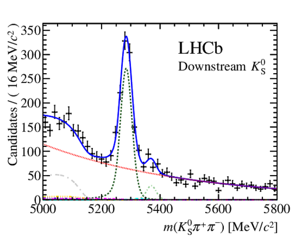
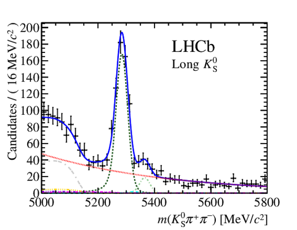
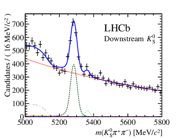
Invariant mass distribution of $ K ^0_{\rm\scriptscriptstyle S} \pi^{+}\pi^{-}$ candidates with the selection requirements for the (top) $\Lambda ^0_ b \rightarrow K ^0_{\rm\scriptscriptstyle S} p h ^- $ , (middle) $\Lambda ^0_ b \rightarrow \Lambda ^+_ c (\rightarrow p K ^0_{\rm\scriptscriptstyle S} ) h ^{-}$ and (bottom) $\Lambda ^0_ b \rightarrow D ^-_ s p $ channels separated into (left) Downstream and (right) Long $ K ^0_{\rm\scriptscriptstyle S}$ categories. Each component of the fit model is displayed: the $ B ^0$ ( $ B ^0_ s $ ) decay is represented by the dashed dark (dot dashed light) green line; the background from $ B ^0_ s \rightarrow K ^0_{\rm\scriptscriptstyle S} K ^\pm \pi ^\mp $ decays by the long dashed cyan line; $ B ^- \rightarrow D ^0 (\rightarrow K ^0_{\rm\scriptscriptstyle S} \pi ^+ \pi ^- ) \pi ^- $ (grey double-dash dotted), charmless $ B ^0$ ( $ B ^+ $ ) decays (orange dash quadruple-dotted), $ B ^0 \rightarrow \eta ^{\prime} (\rho^{0} \gamma) K ^0_{\rm\scriptscriptstyle S} $ (magenta dash double-dotted) and $ B ^0 \rightarrow K ^0_{\rm\scriptscriptstyle S} \pi ^+ \pi ^- \gamma$ (dark violet dash triple-dotted) backgrounds; the overall fit is given by the solid blue line; and the combinatorial background by the dotted red line.

Background-subtracted, efficiency-corrected Dalitz plot distribution of $\Lambda ^0_ b \rightarrow K ^0_{\rm\scriptscriptstyle S} p \pi ^- $ decays for Downstream and Long $ K ^0_{\rm\scriptscriptstyle S}$ categories combined. Some bins have negative entries (consistent with zero) and appear empty.

Animated gif made out of all figures.

Fitted yields and efficiency for each channel, separated by $ K ^0_{\rm\scriptscriptstyle S}$ type. Yields are given with both statistical and systematic uncertainties, whereas for the efficiencies only the uncertainties due to the limited Monte Carlo sample sizes are given. The three rows for the $ B ^0 \rightarrow K ^0_{\rm\scriptscriptstyle S} \pi ^+ \pi ^- $ decay correspond to the different BDT selections for charmless signal modes and the channels containing $\Lambda ^+_ c $ or $ D ^-_ s $ hadrons.

Relative systematic uncertainties on the branching fraction ratios ($\%$) with respect to $ B ^0 \rightarrow K ^0_{\rm\scriptscriptstyle S} \pi ^+ \pi ^- $ decays. The total is obtained from the sum in quadrature of all contributions except that from knowledge of the fragmentation fractions.