Measurement of resonant and $CP$ components in $\overline{B}_s^0\to J/\psi\pi^+\pi^-$ decays

Information

LHCb-PAPER-2013-069
CERN-PH-EP-2014-024
arXiv:1402.6248 [PDF]

(Submitted on 25 Feb 2014)
Phys. Rev. D89 (2014) 092006
Inspire 1282445

Tools

Abstract

The resonant structure of the decay $\overline{B}_s^0\to J/\psi\pi^+\pi^-$ is studied using data corresponding to 3 fb$^{-1}$ of integrated luminosity from $pp$ collisions by the LHC and collected by the LHCb detector. Five interfering $\pi^+\pi^-$ states are required to describe the decay: $f_0(980),f_0(1500),f_0(1790),f_2(1270)$, and $f_2^{\prime}(1525)$. An alternative model including these states and a non-resonant $J/\psi \pi^+\pi^-$ component also provides a good description of the data. Based on the different transversity components measured for the spin-2 intermediate states, the final state is found to be compatible with being entirely $CP$-odd. The $CP$-even part is found to be $<2.3$ at 95 confidence level. The $f_0(500)$ state is not observed, allowing a limit to be set on the absolute value of the mixing angle with the $f_0(980)$ of $<7.7^{\circ}$ at 90 confidence level, consistent with a tetraquark interpretation of the $f_0(980)$ substructure.

Figures and captions

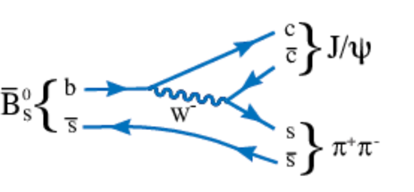
Leading order diagram for $\overline{ B }{} ^0_ s $ decays into $J/\psi \pi^+\pi^-$.	feyn1.pdf [87 KiB] HiDef png [95 KiB] Thumbnail [110 KiB] *.C file
Definition of helicity angles. For details see text.	helAng[..].pdf [26 KiB] HiDef png [68 KiB] Thumbnail [51 KiB] *.C file
Distributions of the BDT classifier for both training and test samples of $ { J \mskip -3mu/\mskip -2mu\psi \mskip 2mu} \pi^+\pi^-$ signal and background events. The signal samples are from simulation and the background samples are from data.	overtr[..].pdf [86 KiB] HiDef png [338 KiB] Thumbnail [320 KiB] *.C file
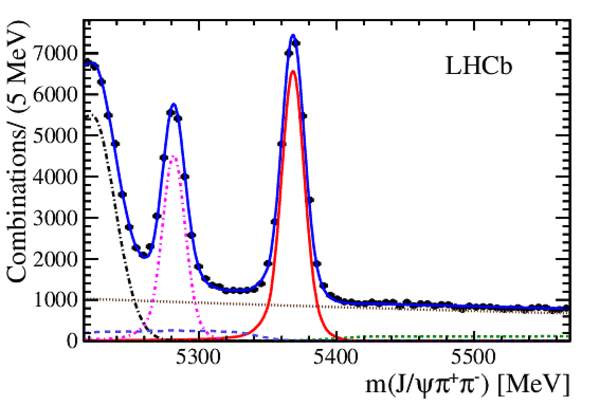
Invariant mass of $J/\psi \pi^+\pi^-$ combinations. The data have been fitted with double Crystal Ball signal and several background functions. The (red) solid curve shows the $\overline{ B }{} ^0_ s $ signal, the (brown) dotted line shows the combinatorial background, the (green) short-dashed line shows the $B^-$ background, the (purple) dot-dashed curve is $\overline{ B }{} ^0 \rightarrow J/\psi \pi^+\pi^-$, the (light blue) long-dashed line is the sum of $\overline{ B }{} ^0_ s \rightarrow J/\psi\eta'$, $\overline{ B }{} ^0_ s \rightarrow J/\psi\phi$ with $\phi\rightarrow \pi^+\pi^-\pi^0$ backgrounds and the $\Lambda _b^0 \rightarrow { J \mskip -3mu/\mskip -2mu\psi \mskip 2mu} K^- p$ reflection, the (black) dot-long dashed curve is the $\overline{ B }{} ^0 \rightarrow J/\psi K^- \pi^+$ reflection and the (blue) solid curve is the total.	fitm-new.pdf [15 KiB] HiDef png [301 KiB] Thumbnail [218 KiB] *.C file
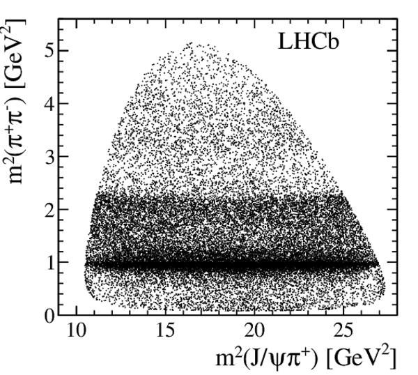
Distribution of $m^2(\pi^+\pi^-)$ versus $m^2(J/\psi\pi^+)$ for all events within $\pm20$ MeV of the $\overline{ B }{} ^0_ s $ mass peak.	dlz.pdf [260 KiB] HiDef png [754 KiB] Thumbnail [308 KiB] *.C file
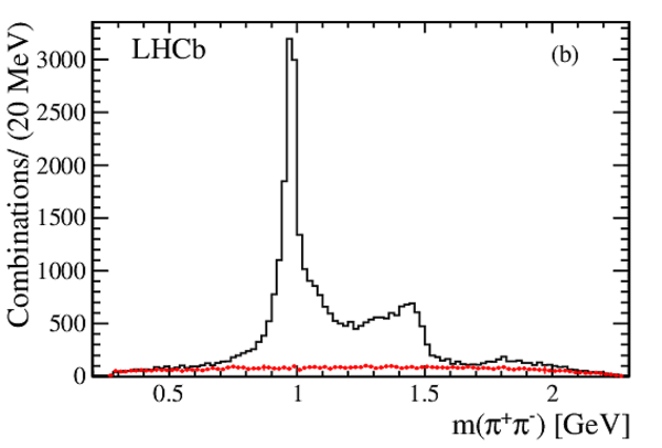
Distributions of (a) $m(J/\psi \pi^+)$ and (b) $m(\pi^+\pi^-)$ for $\overline{ B }{} ^0_ s \rightarrow J/\psi \pi^+\pi^-$ candidate decays within $\pm20$ MeV of the $\overline{ B }{} ^0_ s $ mass. The (red) points with error bars show the background contribution determined from $m(J/\psi \pi^+\pi^-)$ fits performed in each bin of the plotted variables.	mjpsip[..].pdf [12 KiB] HiDef png [136 KiB] Thumbnail [130 KiB] *.C file
	mpp-data.pdf [13 KiB] HiDef png [144 KiB] Thumbnail [134 KiB] *.C file
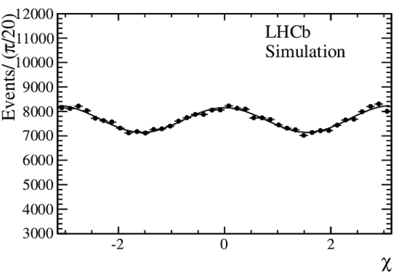
Distribution of the angle $\chi$ for the $J/\psi \pi^+\pi^-$ simulation sample fitted with Eq. (10), used to determine the efficiency parameters.	chi_acc.pdf [12 KiB] HiDef png [104 KiB] Thumbnail [57 KiB] *.C file
Second order polynomial fit to the acceptance parameter $a(m^2_{hh})$ used in Eq. 11.	cosH_acc.pdf [33 KiB] HiDef png [74 KiB] Thumbnail [143 KiB] *.C file
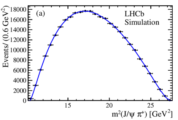
Projections of invariant mass squared of (a) $m^2(J/\psi \pi^+)$ and (b) $m^2(J/\psi \pi^-)$ of the simulated Dalitz plot used to measure the efficiency parameters. The points represent the simulated event distributions and the curves the polynomial fit.	effx.pdf [13 KiB] HiDef png [183 KiB] Thumbnail [167 KiB] *.C file
	effz.pdf [13 KiB] HiDef png [182 KiB] Thumbnail [166 KiB] *.C file
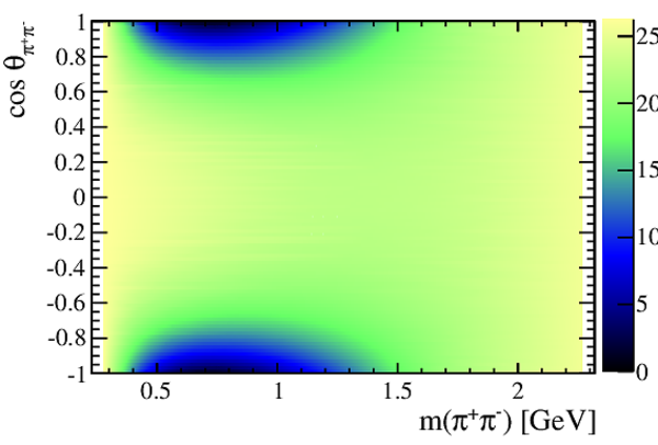
Parameterization of the detection efficiency as a function of $\cos\theta_{\pi^+\pi^-}$ and $m(\pi^+\pi^-)$. The scale is arbitrary.	acc3.pdf [153 KiB] HiDef png [1 MiB] Thumbnail [478 KiB] *.C file
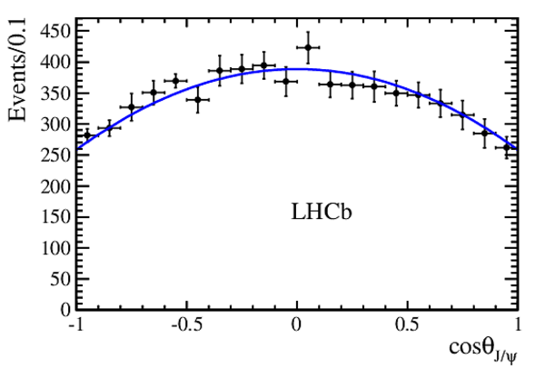
Distribution of $\cos\theta_{J/\psi}$ of the other background and the fitted function $1+\alpha\cos^2\theta_{J/\psi}$. The points with error bars show the background obtained from candidate mass fits in bins of $\cos\theta_{J/\psi}$.	cosH_bkg.pdf [12 KiB] HiDef png [132 KiB] Thumbnail [130 KiB] *.C file
Projections of (a) $\cos\theta_{\pi\pi}$ and (b) $m(\pi^+\pi^-)$ of the total background. The (blue) histogram or curve is projection of the fit, and the points with error bars show the like-sign combinations added with additional $\rho^0$ background.	coshh-bkg.pdf [12 KiB] HiDef png [147 KiB] Thumbnail [147 KiB] *.C file
	mpp-bkg.pdf [12 KiB] HiDef png [178 KiB] Thumbnail [169 KiB] *.C file
Distribution of $\chi$ of the total background and the fitted function. The points with error bars show the like-sign combinations added with additional $\rho^0$ background.	chi_bkg.pdf [12 KiB] HiDef png [135 KiB] Thumbnail [132 KiB] *.C file
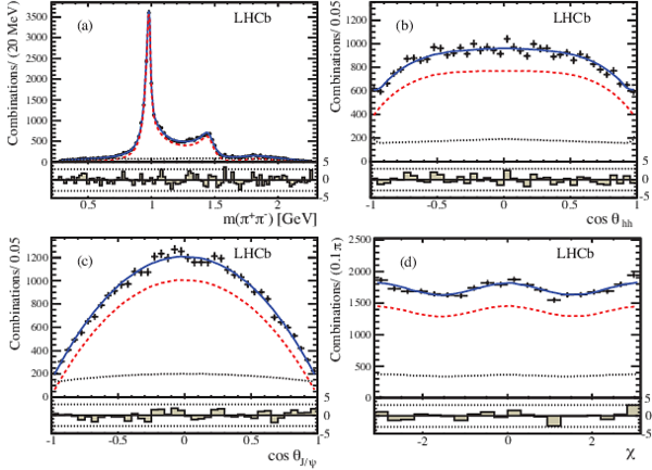
Projections of (a) $m(\pi^+\pi^-)$, (b) $\cos\theta_{\pi\pi}$, (c) $\cos \theta_{J/\psi}$ and (d) $\chi$ for 5R Solution I. The points with error bars are data, the signal fit is shown with a (red) dashed line, the background with a (black) dotted line, and the (blue) solid line represents the total.	5RSol1.pdf [64 KiB] HiDef png [687 KiB] Thumbnail [376 KiB] *.C file
Projections of (a) $m(\pi^+\pi^-)$, (b) $\cos\theta_{\pi\pi}$, (c) $\cos \theta_{J/\psi}$ and (d) $\chi$ for 5R+NR Solution II. The points with error bars are data, the signal fit is shown with a (red) dashed line, the background with a (black) dotted line, and the (blue) solid line represents the total.	5RSol2.pdf [65 KiB] HiDef png [691 KiB] Thumbnail [373 KiB] *.C file
Distribution of $m(\pi^+\pi^-)$ with contributing components labeled from 5R Solution I.	mpp-contr.pdf [18 KiB] HiDef png [305 KiB] Thumbnail [231 KiB] *.C file
Distribution of $m(\pi^+\pi^-)$ with contributing components labeled from 5R+NR Solution II.	mpp-contr2.pdf [18 KiB] HiDef png [330 KiB] Thumbnail [239 KiB] *.C file
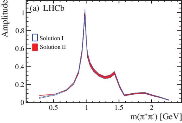
S-wave (a) amplitude strength and (b) phase as a function of $m(\pi^+\pi^-)$ from the 5R Solution I (open) and 5R+NR Solution II (solid), where the widths of the curves reflect $\pm1\sigma$ statistical uncertainties. The reference point is chosen at 980 MeV with amplitude strength equal to 1 and phase equal to 0.	amp.pdf [43 KiB] HiDef png [197 KiB] Thumbnail [148 KiB] *.C file
	ph.pdf [34 KiB] HiDef png [286 KiB] Thumbnail [154 KiB] *.C file
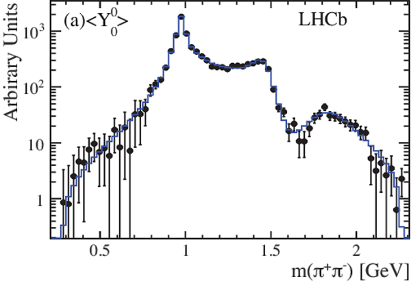
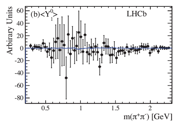
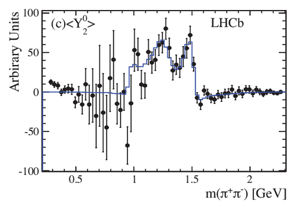
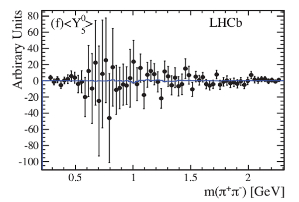
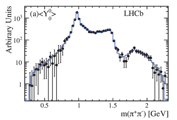
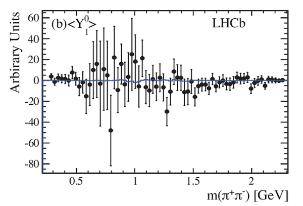
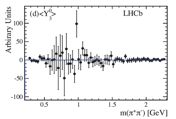
The $\pi^+\pi^-$ mass dependence of the spherical harmonic moments of $\cos \theta_{\pi\pi}$ after efficiency corrections and background subtraction: (a) $\langle Y^0_0\rangle$ ($\chi^2$/ndf =78/70), (b) $\langle Y^0_1\rangle$ ($\chi^2$/ndf =37/70), (c) $\langle Y^0_2\rangle$ ($\chi^2$/ndf =79/70), (d) $\langle Y^0_3\rangle$ ($\chi^2$/ndf =42/70), (e) $\langle Y^0_4\rangle$ ($\chi^2$/ndf =43/70), (f) $\langle Y^0_5\rangle$ ($\chi^2$/ndf =35/70). The points with error bars are the data points and the solid curves are derived from the model 5R Solution I.	shy0-log.pdf [39 KiB] HiDef png [259 KiB] Thumbnail [178 KiB] *.C file
	shy1.pdf [37 KiB] HiDef png [316 KiB] Thumbnail [183 KiB] *.C file
	shy2.pdf [36 KiB] HiDef png [299 KiB] Thumbnail [170 KiB] *.C file
	shy3.pdf [35 KiB] HiDef png [281 KiB] Thumbnail [161 KiB] *.C file
	shy4.pdf [35 KiB] HiDef png [287 KiB] Thumbnail [163 KiB] *.C file
	shy5.pdf [37 KiB] HiDef png [329 KiB] Thumbnail [190 KiB] *.C file
The $\pi^+\pi^-$ mass dependence of the spherical harmonic moments of $\cos \theta_{\pi\pi}$ after efficiency corrections and background subtraction: (a) $\langle Y^0_0\rangle$ ($\chi^2$/ndf =73/70), (b) $\langle Y^0_1\rangle$ ($\chi^2$/ndf =36/70), (c) $\langle Y^0_2\rangle$ ($\chi^2$/ndf =72/70), (d) $\langle Y^0_3\rangle$ ($\chi^2$/ndf =43/70), (e) $\langle Y^0_4\rangle$ ($\chi^2$/ndf =41/70), (f) $\langle Y^0_5\rangle$ ($\chi^2$/ndf =34/70). The points with error bars are the data points and the solid curves are derived from the model 5R+NR Solution II.	shy0-s[..].pdf [35 KiB] HiDef png [286 KiB] Thumbnail [163 KiB] *.C file
	shy1-s2.pdf [37 KiB] HiDef png [317 KiB] Thumbnail [183 KiB] *.C file
	shy2-s2.pdf [37 KiB] HiDef png [302 KiB] Thumbnail [170 KiB] *.C file
	shy3-s2.pdf [35 KiB] HiDef png [279 KiB] Thumbnail [161 KiB] *.C file
	shy4-s2.pdf [35 KiB] HiDef png [287 KiB] Thumbnail [163 KiB] *.C file
	shy5-s2.pdf [37 KiB] HiDef png [328 KiB] Thumbnail [189 KiB] *.C file
Animated gif made out of all figures.	PAPER-2013-069.gif Thumbnail

Tables and captions

$ C P$ parity for different spin resonances. Note that spin-0 only has the transversity component $0$.	Table_1.pdf [39 KiB] HiDef png [36 KiB] Thumbnail [17 KiB] tex code
Possible resonance candidates in the $\overline{ B }{} ^0_ s \rightarrow J/\psi \pi^+\pi^-$ decay mode and their parameters used in the fit.	Table_2.pdf [57 KiB] HiDef png [71 KiB] Thumbnail [32 KiB] tex code
Fit $\rm -ln\mathcal{L}$ and $\chi^2/\text{ndf}$ of different resonance models.	Table_3.pdf [38 KiB] HiDef png [125 KiB] Thumbnail [62 KiB] tex code
Fit fractions (%) of contributing components for both solutions.	Table_4.pdf [54 KiB] HiDef png [176 KiB] Thumbnail [89 KiB] tex code
Non-zero interference fraction (%) for both solutions.	Table_5.pdf [44 KiB] HiDef png [119 KiB] Thumbnail [57 KiB] tex code
Fitted resonance phase differences ($^\circ$).	Table_6.pdf [44 KiB] HiDef png [118 KiB] Thumbnail [57 KiB] tex code
Other fit parameters. The uncertainties are only statistical.	Table_7.pdf [53 KiB] HiDef png [107 KiB] Thumbnail [52 KiB] tex code
Absolute systematic uncertainties for Solution I.	Table_8.pdf [56 KiB] HiDef png [101 KiB] Thumbnail [49 KiB] tex code
Absolute systematic uncertainties for Solution II.	Table_9.pdf [57 KiB] HiDef png [107 KiB] Thumbnail [52 KiB] tex code
Fit fraction ranges taking $1\sigma$ regions for both solutions including systematic uncertainties.	Table_10.pdf [44 KiB] HiDef png [182 KiB] Thumbnail [80 KiB] tex code