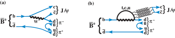
(a) Tree level and (b) penguin diagram for $\overline{ B }{} ^0 $ decays into $J/\psi \pi^+\pi^-$.

Illustration of the three angles used in this analysis.

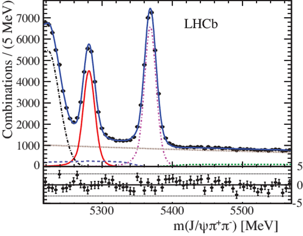
Invariant mass of $J/\psi \pi^+\pi^-$ combinations together with the data fit. The (red) solid curve shows the $\overline{ B }{} ^0 $ signal, the (brown) dotted line shows the combinatorial background, the (green) short-dashed line shows the $B^-$ background, the (purple) dot-dashed curve is $\overline{ B }{} ^0_ s \rightarrow J/\psi \pi^+\pi^-$, the (light blue) long-dashed line is the sum of $\overline{ B }{} ^0_ s \rightarrow J/\psi\eta^{(')}$, $\overline{ B }{} ^0_ s \rightarrow J/\psi\phi$ with $\phi\rightarrow \pi^+\pi^-\pi^0$ backgrounds and the $\Lambda _b^0 \rightarrow { J \mskip -3mu/\mskip -2mu\psi \mskip 2mu} K^- p$ reflection, the (black) dot-long dashed curve is the $\overline{ B }{} ^0 \rightarrow J/\psi K^- \pi^+$ reflection and the (blue) solid curve is the total. The points at the bottom show the difference between the data points and the total fit divided by the statistical uncertainty on the data.

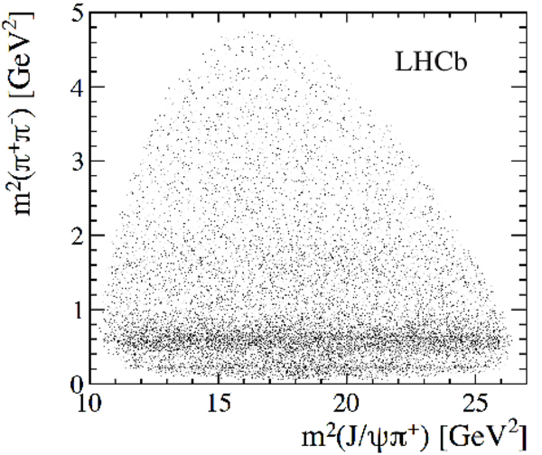
Distribution of $m^2(\pi ^+ \pi ^- )$ versus $m^2( { J \mskip -3mu/\mskip -2mu\psi \mskip 2mu} \pi ^+ )$ for all events within $\pm20$ MeV of the $\overline{ B }{} ^0 $ mass.

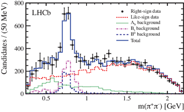
Distributions of (a) $m( { J \mskip -3mu/\mskip -2mu\psi \mskip 2mu} \pi ^+ )$ and (b) $m(\pi ^+ \pi ^- )$ for $\overline{ B }{} ^0 \rightarrow J/\psi\pi^+\pi^-$ candidates within $\pm20$ MeV of the $\overline{ B }{} ^0 $ mass. The red points with error bars show the background contributions obtained by fitting the $m( { J \mskip -3mu/\mskip -2mu\psi \mskip 2mu} \pi ^+ \pi ^- )$ distribution in bins of the plotted variables.

Projections of invariant mass squared (a) $s_{12}\equiv m^2(J/\psi \pi^+)$ and (b) $s_{23}\equiv m^2(\pi^+\pi^-)$ of the simulated Dalitz plot used to measure the efficiency parameters. The points represent the simulated event distributions and the curves the polynomial fit.

The variation of $\varepsilon_1$ is shown as a function of $m(\pi^+\pi^-)$ and $\cos \theta_{\pi^+\pi^-}$.

Distributions of $m(\pi^+\pi^-)$ of background components. The (blue) histogram shows the like-sign combinations added with additional backgrounds using simulations. The (black) points with error bars show the background obtained from the fits to the $m( { J \mskip -3mu/\mskip -2mu\psi \mskip 2mu} \pi ^+ \pi ^- )$ mass spectrum in each bin of $\pi^+\pi^-$ mass.

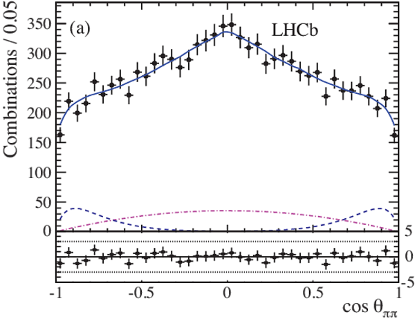
Projections of (a) $\cos \theta_{\pi\pi}$ and (b) $m(\pi ^+ \pi ^- )$ of the background. The points with error bars show the like-sign data combinations added with the $\Lambda ^0_ b $ background and additional simulated backgrounds. The (magenta) dot-dashed line shows the $\eta^{(')}\rightarrow \rho\gamma$ background, the (dark-blue) dashed line the $\overline{ K }{} ^* $ reflection background, and the (blue) solid line the total. The points at the bottom show the difference between the data points and the total fit divided by the statistical uncertainty on the data.

The $\cos\theta_{J/\psi}$ distribution of the data-simulated hybrid background sample. The points with error bars show the like-sign data combinations added with the $\Lambda ^0_ b $ background and additional simulated backgrounds. The (magenta) dot-dashed line shows the $\rho$ background, the (dark-blue) dashed the $\overline{ K }{} ^* $ reflection background and the (blue) solid line the total.

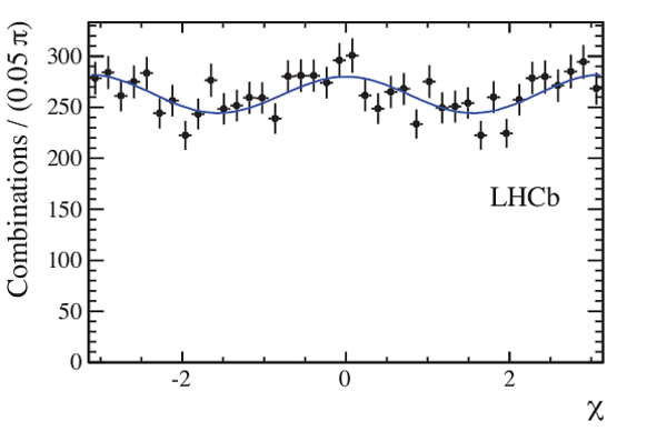
The $\chi$ distribution of the data-simulated hybrid background sample including the $\Lambda ^0_ b $ background and the fitted function $1+p_{b1}\cos \chi + p_{b2} \cos2 \chi$. The $p$-value of this fit is $40\%$.

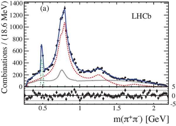
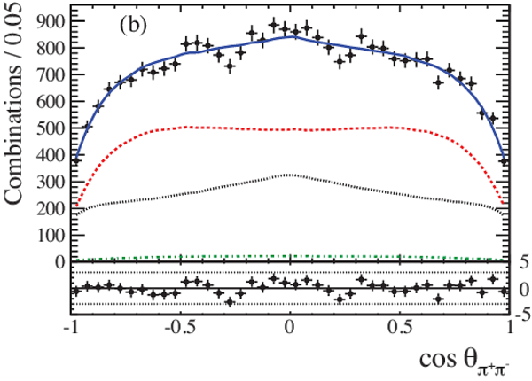
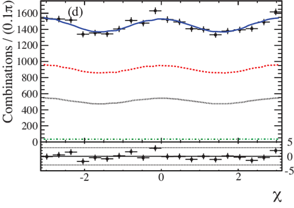
Dalitz fit projections of (a) $m(\pi^+\pi^-)$, (b) $\cos(\theta_{\pi ^+ \pi ^- })$, (c) $\cos \theta_{J/\psi}$ and (d) $\chi$ for the 5R Model + $\rho(1700)$ (Best Model). The points with error bars are data compared with the overall fit, shown by the (blue) solid line. The individual fit components are signal, shown with a (red) dashed line, background, shown with a (black) dotted line, and $ K ^0_{\rm\scriptscriptstyle S} $, shown with a (green) dashed line.

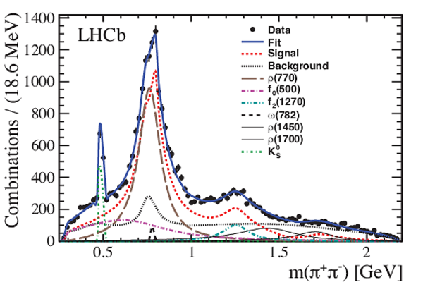
Fit projection of $m(\pi^+\pi^-$) showing the different resonant contributions in the Best Model.

The $\pi^+\pi^-$ mass dependence of the spherical harmonic moments of $\cos \theta_{\pi\pi}$ after efficiency corrections and background subtraction: (a) $\langle Y^0_0\rangle$, (b) $\langle Y^0_1\rangle$, (c) $\langle Y^0_2\rangle$, (d) $\langle Y^0_3\rangle$, (e) $\langle Y^0_4\rangle$, (f) $\langle Y^0_5\rangle$. The errors on the black data points are statistical. The (blue) curves show the fit projections.

Animated gif made out of all figures.

$ C P$ parity of the full final state for different spin resonances. Note that spin-0 only has the 0 transversity component.

Efficiency parameters. There are substantial correlations.

Parameters for the background model.

Possible resonance candidates in the $\overline{ B }{} ^0 \rightarrow J/\psi \pi^+\pi^-$ decay mode.

The $\chi^2/\text{ndf}$ and the $\rm -ln\mathcal{L}$ of different resonance models. The decrease of $\rm -ln\mathcal{L}$ is with respect to the 5R model.

Fit fractions (%) of contributing components for the various models. The uncertainties are statistical only. Sums can differ from 100% due to interference (see Table ???).

Non-zero interference fractions($\%$) obtained from the fit using the Best Model. The uncertainties are statistical only.

The fitted resonant phases from the Best Model. The uncertainties are statistical only.

Fit fractions and transversity fractions of contributing resonances in the Best Model. The first uncertainty is statistical and the second the total systematic.

Branching fractions for each channel. The first uncertainty is statistical and the second the total systematic.

Absolute systematic uncertainties on the results of the amplitude analysis estimated using the Best Model except for the $f_0(980)$ where we use the 7R model.