Feynman diagrams of {\it(left)} $ B ^0 \rightarrow D ^0 K ^{*0} $ and {\it (right)} $ B ^0 \rightarrow \overline{ D }{} {}^0 K ^{*0} $.

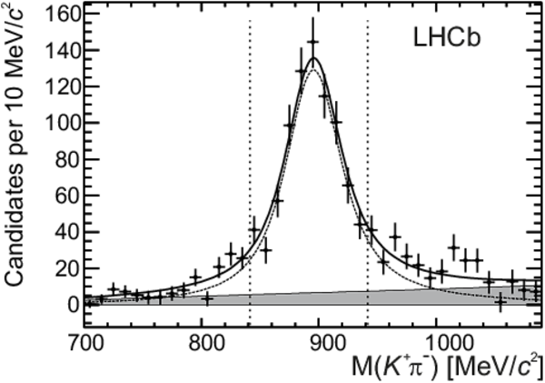
Background-subtracted $ K ^{*0} \rightarrow K ^+ \pi ^- $ invariant mass for $ B ^0 \rightarrow D ( K ^+ \pi ^- ) K ^{*0} $ signal candidates. The data (points) and the fit described in the text (solid line) are shown. The dashed line represents the $ K ^{*0} $ signal and the filled area the non- $ K ^{*0}$ contribution to the $ B ^0 \rightarrow D K ^{*0} $ signal. The vertical dotted lines indicate the invariant mass region used in the analysis.

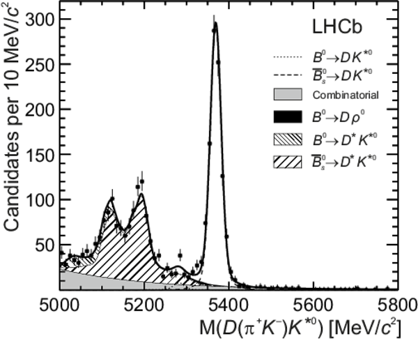
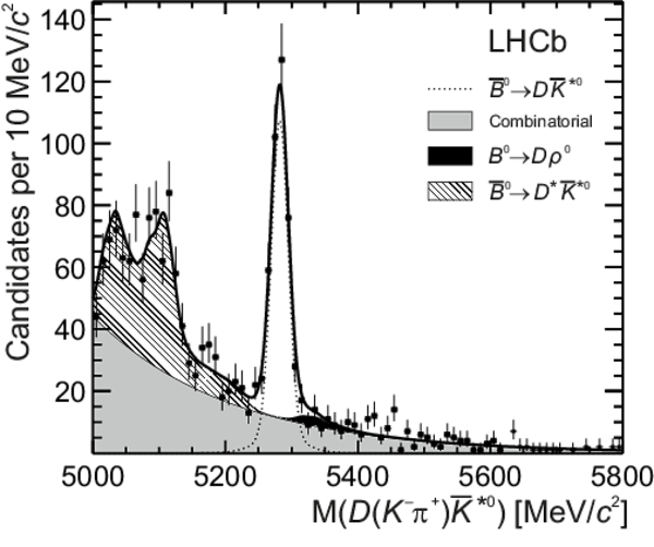
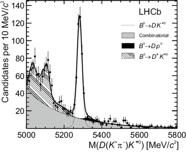
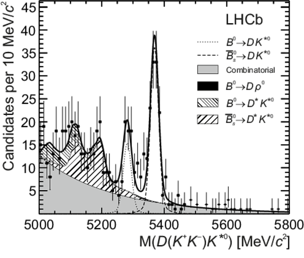
Distributions of (top left) $ D (\pi ^- K ^+ ) \overline{ K }{} {}^{*0} $, (top right) $ D (\pi ^+ K ^- ) K ^{*0} $, (bottom left) $ D ( K ^- \pi ^+ ) \overline{ K }{} {}^{*0} $ and (bottom right) $ D ( K ^+ \pi ^- ) K ^{*0} $ invariant mass. The data (black points) and the fitted invariant mass model (thick solid line) are shown. The PDFs corresponding to the different species are indicated in the legend: the $ B ^0 $ signal, the $ B ^0_ s $ signal, combinatorial background, $ B ^0 \rightarrow D \rho^0$ background, partially reconstructed $ B ^0_ s \rightarrow D ^* \overline{ K }{} {}^{*0} $ and $ B ^0 \rightarrow D ^* K ^{*0} $ backgrounds.

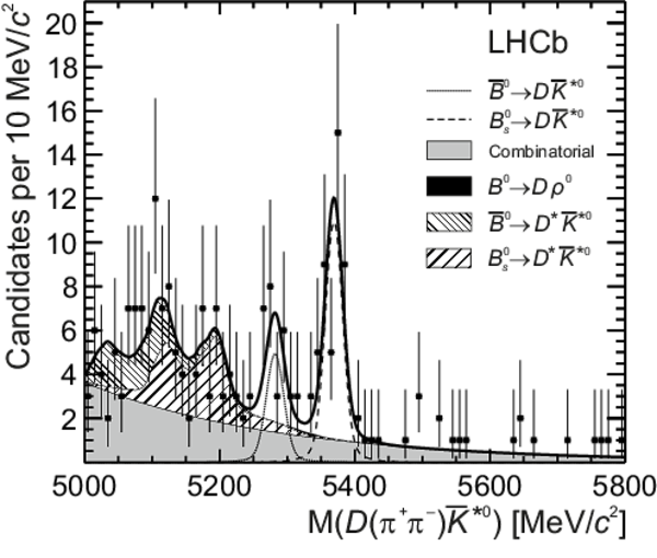
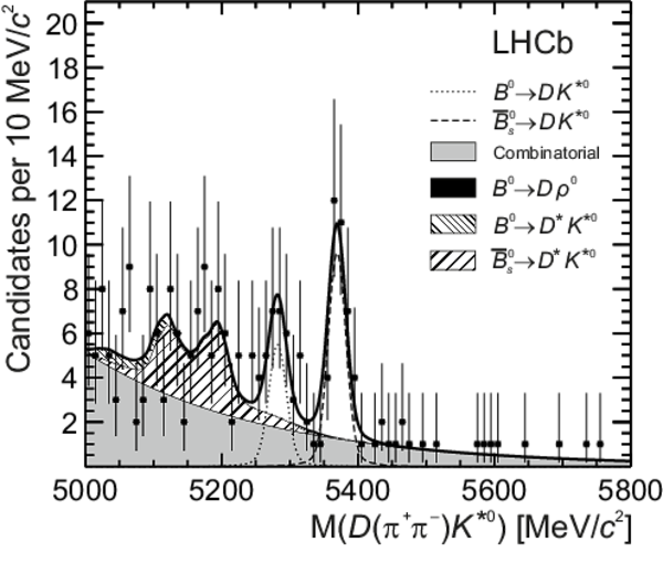
Distributions of (top left) $ D ( K ^+ K ^- ) \overline{ K }{} {}^{*0} $, (top right) $ D ( K ^+ K ^- ) K ^{*0} $, (bottom left) $ D (\pi ^+ \pi ^- ) \overline{ K }{} {}^{*0} $ and (bottom right) $ D (\pi ^+ \pi ^- ) K ^{*0} $ invariant mass. The data (black points) and the fitted invariant mass model (thick solid line) are shown. The PDFs corresponding to the different species are indicated in the legend: the $ B ^0 $ signal, the $ B ^0_ s $ signal, combinatorial background, $ B ^0 \rightarrow D \rho^0$ background and partially reconstructed $ B ^0_ s \rightarrow D ^* \overline{ K }{} {}^{*0} $ and $ B ^0 \rightarrow D ^* K ^{*0} $ backgrounds.

$p$-value as a function of $r_{ B }$, for $\kappa=0.95\pm0.03$. The horizontal dashed lines represent the $1\sigma$ and $2\sigma$ confidence levels and the vertical dotted line represents the obtained central value.

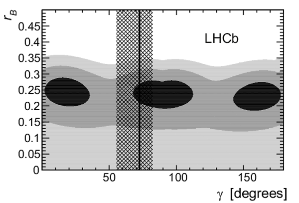
Two-dimensional projections of the $p$-value in $(r_B,\delta_B,\gamma )$ parameter space onto (left) $r_{ B }$ and $\gamma$ and (right) $\delta_{ B }$ and $\gamma$, for $\kappa=0.95\pm0.03$. The contours are the $n\sigma$ profile likelihood contours, where $\Delta\chi^2 = n^2$ with $n = 1$ (black), 2 (medium grey), and 3 (light gray), corresponding to 39.4%, 86.5% and 98.9% confidence level, respectively. The vertical line and hashed band represent the best-fit value of $\gamma $ and the 68.3% confidence level interval by Ref. [3].

Animated gif made out of all figures.

Yields of signal candidates with their statistical uncertainties.

Uncertainties in the observables. All model-related systematic uncertainties are added in quadrature and the result is shown as one source of systematic uncertainty. The presence of `--' indicates that the source of uncertainty does not affect the observable.

Supplementary material full pdf