Measurement of $CP$ asymmetry in $B^0_s \rightarrow D^{\mp}_s K^{\pm}$ decays

Information

LHCb-PAPER-2014-038
CERN-PH-EP-2014-168
arXiv:1407.6127 [PDF]

(Submitted on 23 Jul 2014)
JHEP 11 (2014) 060
Inspire 1307415

Tools

Abstract

We report on measurements of the time-dependent CP violating observables in $B^0_s\rightarrow D^{\mp}_s K^{\pm}$ decays using a dataset corresponding to 1.0 fb$^{-1}$ of pp collisions recorded with the LHCb detector. We find the CP violating observables $C_f=0.53\pm0.25\pm0.04$, $A^{\Delta\Gamma}_f=0.37\pm0.42\pm0.20$, $A^{\Delta\Gamma}_{\bar{f}}=0.20\pm0.41\pm0.20$, $S_f=-1.09\pm0.33\pm0.08$, $S_{\bar{f}}=-0.36\pm0.34\pm0.08$, where the uncertainties are statistical and systematic, respectively. Using these observables together with a recent measurement of the $B^0_s$ mixing phase $-2\beta_s$ leads to the first extraction of the CKM angle $\gamma$ from $B^0_s \rightarrow D^{\mp}_s K^{\pm}$ decays, finding $\gamma$ = (115$_{-43}^{+28}$)$^\circ$ modulo 180$^\circ$ at 68 CL, where the error contains both statistical and systematic uncertainties.

Figures and captions

Feynman diagrams for $\overline{ B }{} {}^0_ s \rightarrow D_{\hspace{-0.0625em}s} ^+ K^-$ without (left) and with (right) $ B ^0_ s $ mixing.	Fig1a.pdf [11 KiB] HiDef png [24 KiB] Thumbnail [14 KiB] *.C file
	Fig1b.pdf [13 KiB] HiDef png [36 KiB] Thumbnail [22 KiB] *.C file
Mass distributions for $ D ^-_ s $ candidates passing (black, open circles) and failing (red, crosses) the PID selection criteria. In reading order: $ D ^-_ s \rightarrow K ^- K ^+ \pi ^- $ , $ D ^-_ s \rightarrow \pi ^- \pi ^+ \pi ^- $ , and $ D ^-_ s \rightarrow K ^- \pi ^+ \pi ^- $ .	Fig2a.pdf [34 KiB] HiDef png [211 KiB] Thumbnail [175 KiB] *.C file
	Fig2b.pdf [47 KiB] HiDef png [252 KiB] Thumbnail [209 KiB] *.C file
	Fig2c.pdf [27 KiB] HiDef png [212 KiB] Thumbnail [173 KiB] *.C file
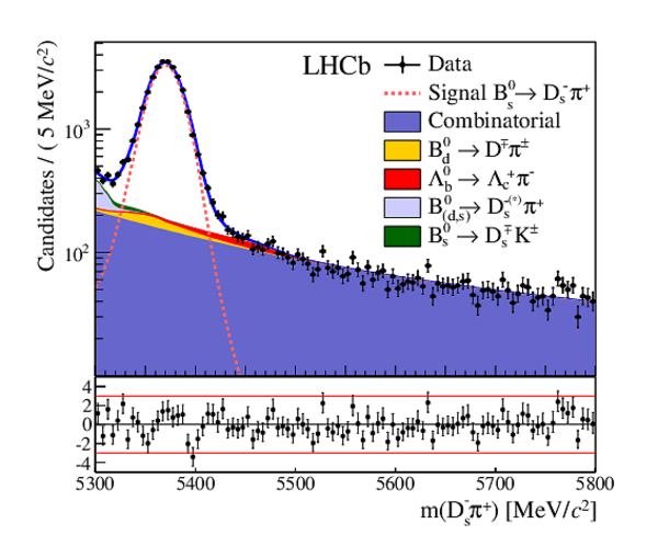
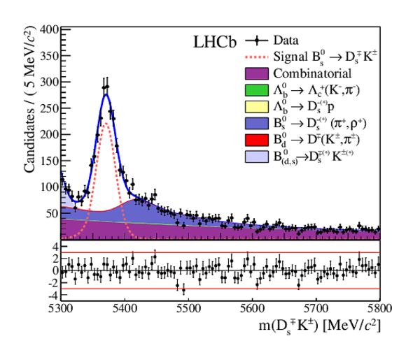
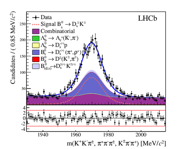
The multivariate fit to the (left) $ B ^0_ s \rightarrow D ^-_ s \pi ^+ $ and (right) $ B ^0_ s \rightarrow D_{\hspace{-0.0625em}s} ^\mp K^\pm$ candidates for all $ D ^-_ s $ decay modes combined. From top to bottom: distributions of candidates in $ B ^0_ s $ mass, $ D ^-_ s $ mass, companion PID log-likelihood difference. The solid, blue, line represents the sum of the fit components.	Fig3a.pdf [42 KiB] HiDef png [353 KiB] Thumbnail [280 KiB] *.C file
	Fig3d.pdf [43 KiB] HiDef png [398 KiB] Thumbnail [305 KiB] *.C file
	Fig3b.pdf [42 KiB] HiDef png [345 KiB] Thumbnail [278 KiB] *.C file
	Fig3e.pdf [42 KiB] HiDef png [407 KiB] Thumbnail [313 KiB] *.C file
	Fig3c.pdf [38 KiB] HiDef png [314 KiB] Thumbnail [245 KiB] *.C file
	Fig3f.pdf [39 KiB] HiDef png [376 KiB] Thumbnail [298 KiB] *.C file
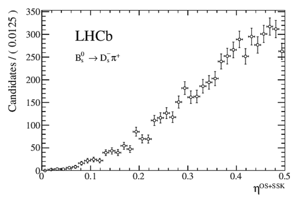
Measured mistag rate against the average predicted mistag rate for the (left) OS and (right) SSK taggers in $ B ^0_ s \rightarrow D ^-_ s \pi ^+ $ decays. The error bars represent only the statistical uncertainties. The solid curve is the linear fit to the data points, the shaded area defines the 68% confidence level region of the calibration function (statistical only).	Fig4a.pdf [9 KiB] HiDef png [113 KiB] Thumbnail [91 KiB] *.C file
	Fig4b.pdf [9 KiB] HiDef png [116 KiB] Thumbnail [95 KiB] *.C file
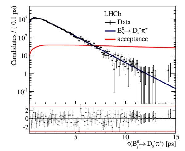
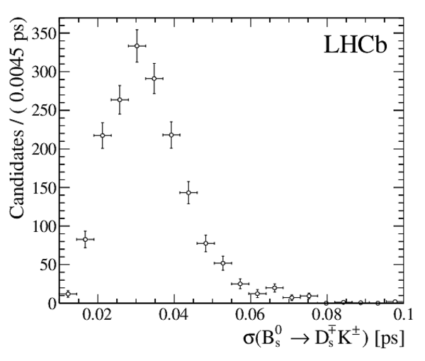
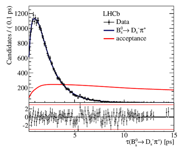
Result of the \it sFit to the decay-time distribution of $ B ^0_ s \rightarrow D ^-_ s \pi ^+ $ candidates, which is used to measure the decay-time acceptance in $ B ^0_ s \rightarrow D_{\hspace{-0.0625em}s} ^\mp K^\pm$ decays. The solid curve is measured decay-time acceptance.	Fig5.pdf [43 KiB] HiDef png [249 KiB] Thumbnail [225 KiB] *.C file
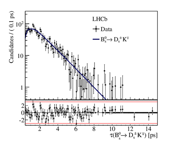
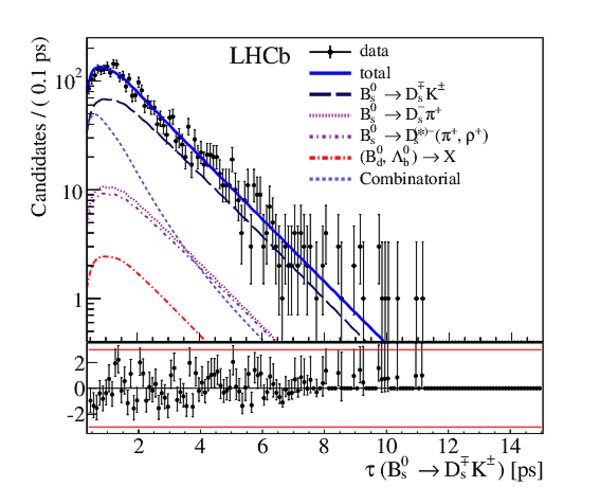
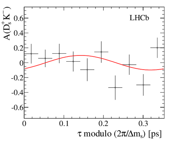
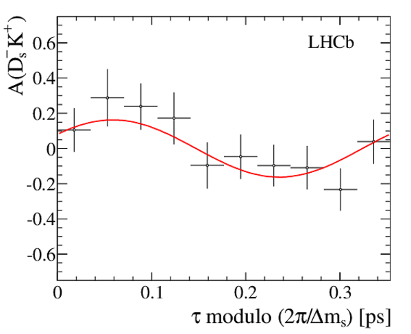
Result of the decay-time (top left) \it sFit and (top right) \it cFit to the $ B ^0_ s \rightarrow D_{\hspace{-0.0625em}s} ^\mp K^\pm$ candidates; the \it cFit plot groups $ B ^0_ s \rightarrow D ^{-}_ s \pi ^+ $ and $ B ^0_ s \rightarrow D ^-_ s \rho^{+}$ , and also groups $ B ^0 \rightarrow D ^- K ^+ $ , $ B ^0 \rightarrow D ^- \pi ^+ $ , $\overline{\Lambda} {}^0_ b \rightarrow \overline{\Lambda} {}^-_ c K ^+ $ , $\overline{\Lambda} {}^0_ b \rightarrow \overline{\Lambda} {}^-_ c \pi ^+ $ , $\Lambda ^0_ b \rightarrow D ^-_ s p$ , $\Lambda ^0_ b \rightarrow D ^{-}_ s p$ , and $ B ^0 \rightarrow D ^-_ s K ^+ $ together for the sake of clarity. The folded asymmetry plots for (bottom left) $ D ^+_ s K^-$, and (bottom right) $ D ^-_ s K^+$ are also shown.	Fig6a.pdf [28 KiB] HiDef png [219 KiB] Thumbnail [197 KiB] *.C file
	Fig6b.pdf [108 KiB] HiDef png [320 KiB] Thumbnail [263 KiB] *.C file
	Fig6c.pdf [9 KiB] HiDef png [125 KiB] Thumbnail [114 KiB] *.C file
	Fig6d.pdf [9 KiB] HiDef png [127 KiB] Thumbnail [115 KiB] *.C file
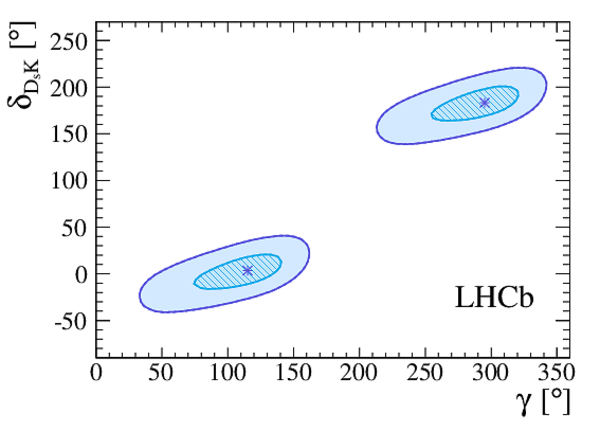
Graph showing $ 1-{\rm CL}$ for $\gamma$ , together with the central value and the 68.3% CL interval as obtained from the frequentist method described in the text (top). Profile likelihood contours of $ r_{ D_{\hspace{-0.0625em}s} \hspace{-0.0625em} K }$ vs. $\gamma$ (bottom left), and $\delta$ vs. $\gamma$ (bottom right). The contours are the $1\sigma$ ($2\sigma$) profile likelihood contours, where $\Delta\chi^2=1$ $(\Delta\chi^2=4)$, corresponding to 39% CL (86% CL) in Gaussian approximation. The markers denote the best-fit values.	Fig7a.pdf [8 KiB] HiDef png [204 KiB] Thumbnail [158 KiB] *.C file
	Fig7b.pdf [9 KiB] HiDef png [298 KiB] Thumbnail [194 KiB] *.C file
	Fig7c.pdf [9 KiB] HiDef png [239 KiB] Thumbnail [160 KiB] *.C file
Animated gif made out of all figures.	PAPER-2014-038.gif Thumbnail

Tables and captions

Calibration parameters of the combined OS tagger extracted from different control channels. In each entry the first uncertainty is statistical and the second systematic.	Table_1.pdf [52 KiB] HiDef png [77 KiB] Thumbnail [37 KiB] tex code
Flavour tagging performance for the three different tagging categories for $ B ^0_ s \rightarrow D ^-_ s \pi ^+ $ candidates.	Table_2.pdf [37 KiB] HiDef png [65 KiB] Thumbnail [32 KiB] tex code
Fitted values of the $ C P$ observables to the $ B ^0_ s \rightarrow D_{\hspace{-0.0625em}s} ^\mp K^\pm$ time distribution for (left) \it sFit and (right) \it cFit , where the first uncertainty is statistical, the second is systematic. All parameters other than the $ C P$ observables are constrained in the fit.	Table_3.pdf [52 KiB] HiDef png [70 KiB] Thumbnail [37 KiB] tex code
Statistical correlation matrix of the $ B ^0_ s \rightarrow D_{\hspace{-0.0625em}s} ^\mp K^\pm$ (top) \it sFit and (bottom) {\it cFit } $ C P$ parameters. Other fit parameters have negligible correlations with the $ C P$ parameters and are omitted for brevity.	Table_4.pdf [51 KiB] HiDef png [83 KiB] Thumbnail [38 KiB] tex code
Systematic errors, relative to the statistical error, for (top) \it sFit and (bottom) \it cFit . The daggered contributions ( $\Gamma_{ s }$ , $\Delta\Gamma_{ s }$ ) are given separately for comparison (see text) with the other uncertainties and are not added in quadrature to produce the total.	Table_5.pdf [54 KiB] HiDef png [153 KiB] Thumbnail [63 KiB] tex code
Systematic uncertainty correlations for (top) \it sFit and (bottom) \it cFit .	Table_6.pdf [51 KiB] HiDef png [81 KiB] Thumbnail [40 KiB] tex code

Supplementary Material [file]

Supplementary material full pdf	supple[..].pdf [518 KiB]
This ZIP file contains supplemetary material for the publication LHCb-PAPER-2014-038. The files are: supplementary.pdf : An overview of the extra figures .pdf, .png, .jpg, .eps, .root, .C: The figures in variuous formats	Fig1a.pdf [16 KiB] HiDef png [94 KiB] Thumbnail [50 KiB] *C file
	Fig1b.pdf [16 KiB] HiDef png [99 KiB] Thumbnail [51 KiB] *C file
	Fig2a.pdf [18 KiB] HiDef png [109 KiB] Thumbnail [57 KiB] *C file
	Fig2b.pdf [17 KiB] HiDef png [94 KiB] Thumbnail [46 KiB] *C file
	Fig2c.pdf [18 KiB] HiDef png [105 KiB] Thumbnail [55 KiB] *C file
	Fig3a.pdf [18 KiB] HiDef png [181 KiB] Thumbnail [147 KiB] *C file
	Fig3b.pdf [18 KiB] HiDef png [171 KiB] Thumbnail [143 KiB] *C file
	Fig3c.pdf [17 KiB] HiDef png [167 KiB] Thumbnail [134 KiB] *C file
	Fig3d.pdf [17 KiB] HiDef png [163 KiB] Thumbnail [137 KiB] *C file
	Fig4a.pdf [15 KiB] HiDef png [104 KiB] Thumbnail [54 KiB] *C file
	Fig4b.pdf [15 KiB] HiDef png [109 KiB] Thumbnail [59 KiB] *C file
	Fig5a.pdf [47 KiB] HiDef png [247 KiB] Thumbnail [211 KiB] *C file
	Fig5b.pdf [43 KiB] HiDef png [249 KiB] Thumbnail [225 KiB] *C file
	Fig6a.pdf [24 KiB] HiDef png [205 KiB] Thumbnail [153 KiB] *C file
	Fig6b.pdf [24 KiB] HiDef png [207 KiB] Thumbnail [155 KiB] *C file
	Fig6c.pdf [26 KiB] HiDef png [177 KiB] Thumbnail [140 KiB] *C file
	Fig6d.pdf [26 KiB] HiDef png [178 KiB] Thumbnail [137 KiB] *C file
	Fig7a.pdf [18 KiB] HiDef png [120 KiB] Thumbnail [60 KiB] *C file
	Fig7b.pdf [19 KiB] HiDef png [138 KiB] Thumbnail [69 KiB] *C file
	Fig8.pdf [15 KiB] HiDef png [320 KiB] Thumbnail [215 KiB] *C file
	Fig9.pdf [152 KiB] HiDef png [414 KiB] Thumbnail [315 KiB] *C file