Measurement of the CKM angle $\gamma$ using $B^\pm \to D K^\pm$ with $D \to K^0_{\rm S} \pi^+\pi^-, K^0_{\rm S} K^+ K^-$ decays

Information

LHCb-PAPER-2014-041
CERN-PH-EP-2014-202
arXiv:1408.2748 [PDF]

(Submitted on 12 Aug 2014)
JHEP 10 (2014) 097
Inspire 1310654

Tools

Abstract

A binned Dalitz plot analysis of $B^\pm \to D K^\pm$ decays, with $D \to K_S \pi^+\pi^-$ and $D \to K_S K^+ K^-$, is performed to measure the \CP-violating observables $x_{\pm}$ and $y_{\pm}$, which are sensitive to the Cabibbo-Kobayashi-Maskawa angle $\gamma$. The analysis exploits a sample of proton-proton collision data corresponding to 3.0\invfb collected by the LHCb experiment. Measurements from CLEO-c of the variation of the strong-interaction phase of the $D$ decay over the Dalitz plot are used as inputs. The values of the parameters are found to be $x_+ = (-7.7 \pm 2.4 \pm 1.0 \pm 0.4)\times 10^{-2}$, $x_- = (2.5 \pm 2.5 \pm 1.0 \pm 0.5) \times 10^{-2}$, $y_+ = (-2.2 \pm 2.5 \pm 0.4 \pm 1.0)\times 10^{-2}$, and $y_- = (7.5 \pm 2.9 \pm 0.5 \pm 1.4) \times 10^{-2}$. The first, second, and third uncertainties are the statistical, the experimental systematic, and that associated with the precision of the strong-phase parameters. These are the most precise measurements of these observables and correspond to $\gamma = (62^{ +15}_{ -14})^\circ$, with a second solution at $\gamma \to \gamma + 180^\circ$, and $r_B = 0.080^{+ 0.019}_{-0.021}$, where $r_B$ is the ratio between the suppressed and favoured $B$ decay amplitudes.

Figures and captions

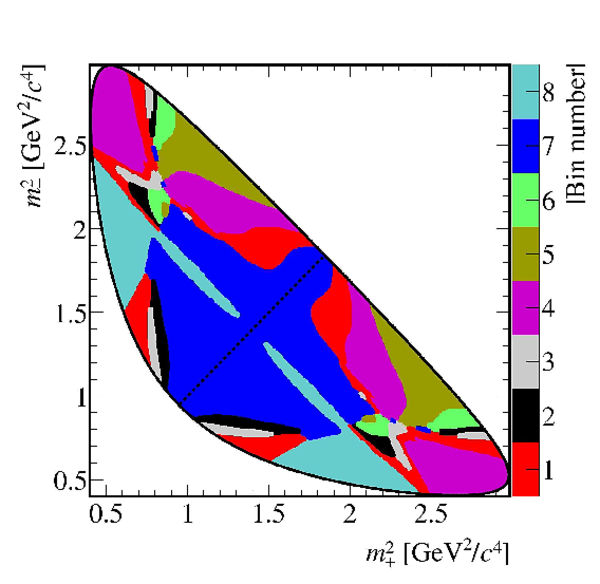
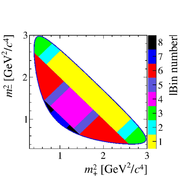
Binning schemes for (left) $ D \rightarrow K ^0_{\rm\scriptscriptstyle S} \pi ^+ \pi ^- $ and (right) $ D \rightarrow K ^0_{\rm\scriptscriptstyle S} K ^+ K ^- $ . The diagonal line separates the positive and negative bins, where the positive bins are in the region where $m^2_->m^2_+$ is satisfied.	KsPiPi[..].pdf [217 KiB] HiDef png [1 MiB] Thumbnail [332 KiB] *.C file
	KsKK2b[..].pdf [214 KiB] HiDef png [779 KiB] Thumbnail [255 KiB] *.C file
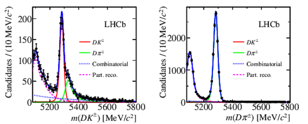
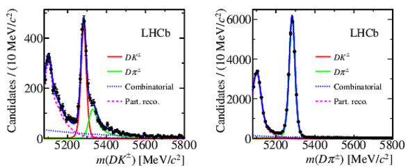
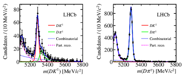
Invariant mass distributions of (left) $ B ^\pm \rightarrow D K ^\pm $ and (right) $ B ^\pm \rightarrow D \pi ^\pm $ candidates, with $ D \rightarrow K ^0_{\rm\scriptscriptstyle S} \pi ^+ \pi ^- $ , divided between the (top) long and (bottom) downstream $ K ^0_{\rm\scriptscriptstyle S}$ categories. Fit results, including the signal and background components, are superimposed.	canvas[..].pdf [28 KiB] HiDef png [238 KiB] Thumbnail [168 KiB] *.C file
	canvas[..].pdf [28 KiB] HiDef png [236 KiB] Thumbnail [167 KiB] *.C file
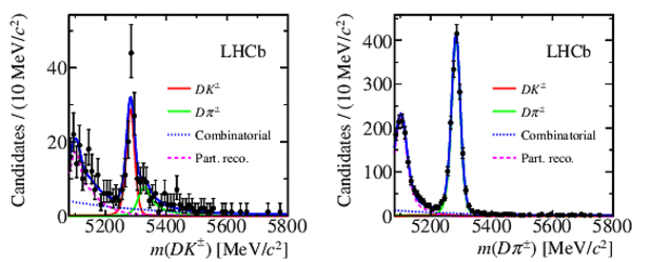
Invariant mass distributions of (left) $ B ^\pm \rightarrow D K ^\pm $ and (right) $ B ^\pm \rightarrow D \pi ^\pm $ candidates, with $ D \rightarrow K ^0_{\rm\scriptscriptstyle S} K ^+ K ^- $ , divided between the (top) long and (bottom) downstream $ K ^0_{\rm\scriptscriptstyle S}$ categories. Fit results, including the signal and background components, are superimposed.	canvas[..].pdf [28 KiB] HiDef png [239 KiB] Thumbnail [173 KiB] *.C file
	canvas[..].pdf [28 KiB] HiDef png [247 KiB] Thumbnail [180 KiB] *.C file
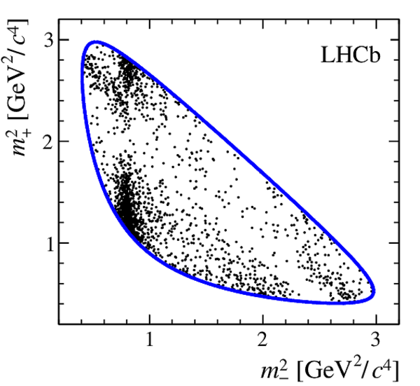
Dalitz plots of $ B ^\pm \rightarrow D K ^\pm $ candidates in the signal region for $ D \rightarrow K ^0_{\rm\scriptscriptstyle S} \pi ^+ \pi ^- $ decays from (left) $ B ^+ $ and (right) $ B ^- $ decays. Both long and downstream $ K ^0_{\rm\scriptscriptstyle S}$ candidates are included. The blue line indicates the kinematic boundary.	Dalitz[..].pdf [432 KiB] HiDef png [290 KiB] Thumbnail [276 KiB] *.C file
	Dalitz[..].pdf [422 KiB] HiDef png [288 KiB] Thumbnail [274 KiB] *.C file
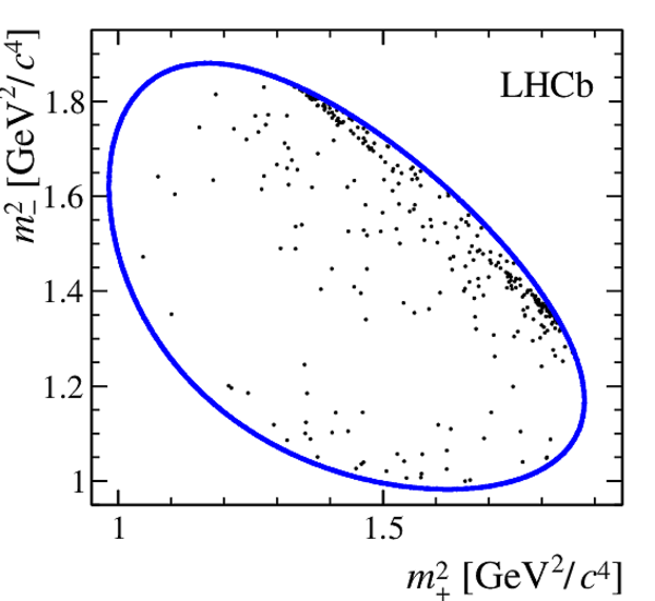
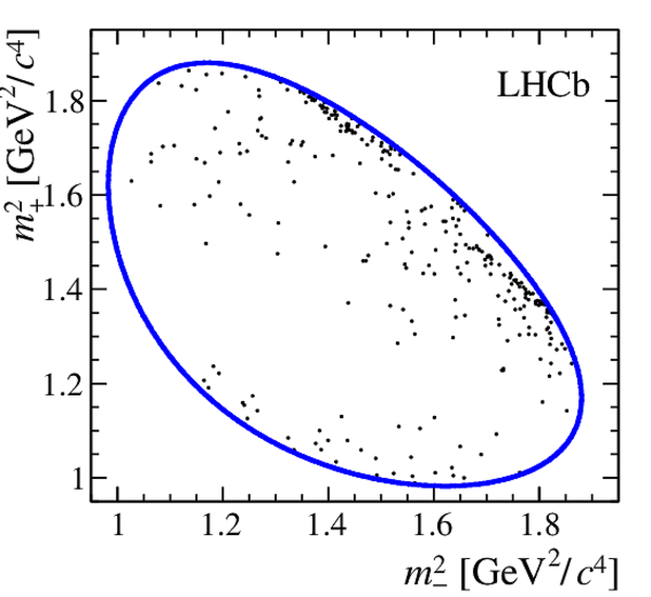
Dalitz plots of $ B ^\pm \rightarrow D K ^\pm $ candidates in the signal region for $ D \rightarrow K ^0_{\rm\scriptscriptstyle S} K ^+ K ^- $ decays from (left) $ B ^+ $ and (right) $ B ^- $ decays. Both long and downstream $ K ^0_{\rm\scriptscriptstyle S}$ candidates are included. The blue line indicates the kinematic boundary.	Dalitz[..].pdf [129 KiB] HiDef png [180 KiB] Thumbnail [163 KiB] *.C file
	Dalitz[..].pdf [129 KiB] HiDef png [191 KiB] Thumbnail [178 KiB] *.C file
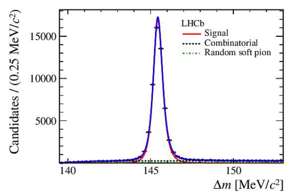
Result of the simultaneous fit to $\optbar{ B}{} \rightarrow D ^{\pm} \mu^\mp\optbarlowcase{\nu}{} _{ \mu}$ , $ D ^ \pm\rightarrow \optbar{ D}{} ^0(\rightarrow K ^0_{\rm\scriptscriptstyle S} \pi ^+ \pi ^- )\pi ^\pm $ decays with downstream $ K ^0_{\rm\scriptscriptstyle S}$ candidates, in 2012 data. A two-dimensional fit is performed in (left) $m( K ^0_{\rm\scriptscriptstyle S} h ^+ h ^- )$ and (right) $\Delta m$. The (blue) total fit PDF is constructed from (solid red) signal, (dashed black) combinatorial background and (dotted green) random soft pion background.	md0_d2[..].pdf [23 KiB] HiDef png [236 KiB] Thumbnail [183 KiB] *.C file
	del_d2[..].pdf [20 KiB] HiDef png [191 KiB] Thumbnail [143 KiB] *.C file
Example efficiency profiles of (left) $ B ^\pm \rightarrow D \pi ^\pm $ and (right) $\optbar{ B}{} \rightarrow D ^{*\pm} \mu^\mp\optbarlowcase{\nu}{} _{ \mu}$ decays in simulation. These plots refer to downstream $ K ^0_{\rm\scriptscriptstyle S}$ candidates under 2012 data taking conditions.	DpiMCprof.pdf [15 KiB] HiDef png [186 KiB] Thumbnail [197 KiB] *.C file
	DmuMCprof.pdf [15 KiB] HiDef png [187 KiB] Thumbnail [199 KiB] *.C file
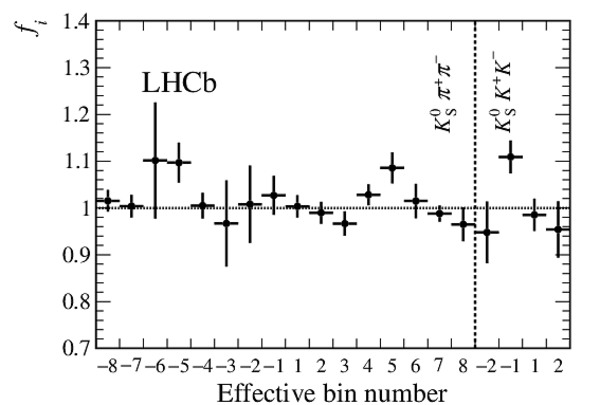
Fractional yield ratios of $ B ^\pm \rightarrow D \pi ^\pm $ to $\optbar{ B}{} \rightarrow D ^{*\pm} \mu^\mp\optbarlowcase{\nu}{} _{ \mu}$ decays, $f_i$, for each effective Dalitz plot bin. The vertical dashed line separates the ratios for $ K ^0_{\rm\scriptscriptstyle S} \pi ^+ \pi ^- $ (bins $-8$ to 8) and $ K ^0_{\rm\scriptscriptstyle S} K ^+ K ^- $ (bins $-2$ to 2). The left (right) plot shows the values of $f_i$ before (after) correcting for the efficiency differences.	before.pdf [15 KiB] HiDef png [101 KiB] Thumbnail [63 KiB] *.C file
	after.pdf [15 KiB] HiDef png [101 KiB] Thumbnail [64 KiB] *.C file
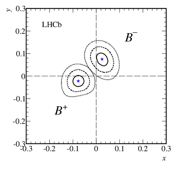
Confidence levels at 39.3%, 86.5% and 98.9% probability for $(x_+,y_+)$ and $(x_{-}, y_{-})$ as measured in $B^\pm \rightarrow D K^\pm$ decays (statistical uncertainties only). The parameters $(x_+,y_+)$ relate to $ B ^+ $ decays and $(x_{-}, y_{-})$ refer to $ B ^- $ decays. The stars represent the best fit central values.	likesc[..].pdf [16 KiB] HiDef png [148 KiB] Thumbnail [147 KiB] *.C file
Combinations of signal yields (data points) in effective bins compared with prediction of $(x_\pm, y_\pm)$ fit (solid histogram) for $ D \rightarrow K ^0_{\rm\scriptscriptstyle S} \pi ^+ \pi ^- $ and $ D \rightarrow K ^0_{\rm\scriptscriptstyle S} K ^+ K ^- $ decays. The dotted histograms give the prediction for $x_\pm=y_\pm=0$. The left plot shows the sum of $B^+$ and $B^-$ yields and the right plot shows the difference of $B^+$ and $B^-$ yields.	sumBpB[..].pdf [15 KiB] HiDef png [135 KiB] Thumbnail [81 KiB] *.C file
	diffBp[..].pdf [15 KiB] HiDef png [134 KiB] Thumbnail [76 KiB] *.C file
The rectangular binning schemes for the two decays. On the left (right) is plotted the scheme for the $ K ^0_{\rm\scriptscriptstyle S} \pi ^+ \pi ^- $ ( $ K ^0_{\rm\scriptscriptstyle S} K ^+ K ^- $ ) decay.	kspp_r[..].pdf [197 KiB] HiDef png [717 KiB] Thumbnail [228 KiB] *.C file
	kspp_k[..].pdf [196 KiB] HiDef png [684 KiB] Thumbnail [222 KiB] *.C file
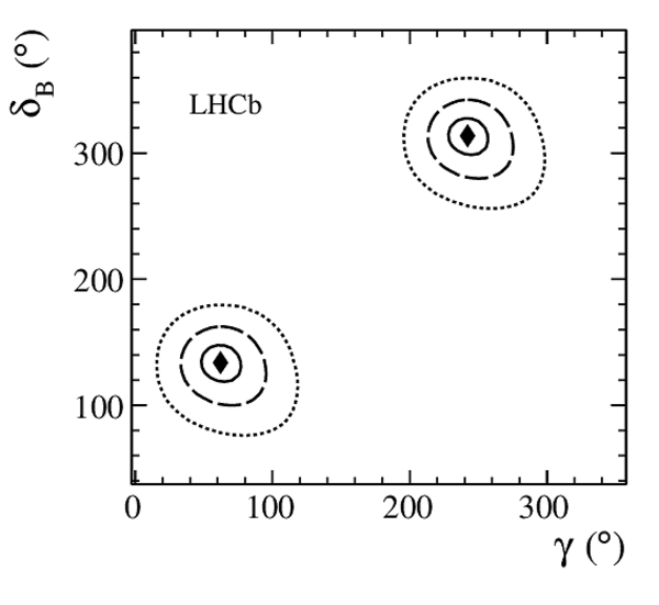
The three-dimensional confidence volumes, corresponding to 19.9%, 73.9% and 97.1% confidence levels, are projected onto the $(\gamma, r_B)$ and $(\gamma, \delta_B)$ planes. The confidence levels are given by solid, dashed and dotted contours. The diamonds mark the central values.	fr_con[..].pdf [14 KiB] HiDef png [115 KiB] Thumbnail [65 KiB] *.C file
	fd_con[..].pdf [15 KiB] HiDef png [97 KiB] Thumbnail [53 KiB] *.C file
Animated gif made out of all figures.	PAPER-2014-041.gif Thumbnail

Tables and captions

Yields and statistical uncertainties in the signal region from the invariant mass fits, scaled from the full fit mass range, for candidates passing the $ B ^\pm \rightarrow D ( K ^0_{\rm\scriptscriptstyle S} \pi ^+ \pi ^- ) h ^\pm$ selection. Values are shown separately for candidates formed using long and downstream $ K ^0_{\rm\scriptscriptstyle S}$ decays. The signal region is between 5247 $ {\mathrm{ Me V /}c^2}$ and 5317 $ {\mathrm{ Me V /}c^2}$ and the full fit range is between 5080 $ {\mathrm{ Me V /}c^2}$ and 5800 $ {\mathrm{ Me V /}c^2}$ .	Table_1.pdf [39 KiB] HiDef png [49 KiB] Thumbnail [22 KiB] tex code
Yields and statistical uncertainties in the signal region from the invariant mass fits, scaled from the full fit mass range, for candidates passing the $ B ^\pm \rightarrow D ( K ^0_{\rm\scriptscriptstyle S} K ^+ K ^- ) h ^\pm$ selection. Values are shown separately for candidates formed using long and downstream $ K ^0_{\rm\scriptscriptstyle S}$ decays. The signal region is between 5247 $ {\mathrm{ Me V /}c^2}$ and 5317 $ {\mathrm{ Me V /}c^2}$ and the full fit range is between 5080 $ {\mathrm{ Me V /}c^2}$ and 5800 $ {\mathrm{ Me V /}c^2}$ .	Table_2.pdf [39 KiB] HiDef png [48 KiB] Thumbnail [22 KiB] tex code
Results for $x_{\pm}$ and $y_{\pm}$ from fits of both the $D \rightarrow K ^0_{\rm\scriptscriptstyle S} \pi^+\pi^-$ and $D \rightarrow K ^0_{\rm\scriptscriptstyle S} K^+K^-$ samples, and from fits of the $D \rightarrow K ^0_{\rm\scriptscriptstyle S} \pi^+\pi^-$ sample only. The first, second, and third uncertainties are the statistical, the experimental systematic, and the error associated with the precision of the strong-phase parameters, respectively.	Table_3.pdf [52 KiB] HiDef png [50 KiB] Thumbnail [29 KiB] tex code
Summary of statistical, experimental, and strong-phase, uncertainties on $x_\pm$ and $y_\pm$ in the case where both $ D \rightarrow K ^0_{\rm\scriptscriptstyle S} \pi ^+ \pi ^- $ and $ D \rightarrow K ^0_{\rm\scriptscriptstyle S} K ^+ K ^- $ decays are included in the fit. All entries are given in multiples of $10^{-2}$.	Table_4.pdf [49 KiB] HiDef png [80 KiB] Thumbnail [36 KiB] tex code
Correlation matrix between the $ x_{\pm}$ , $ y_{\pm}$ parameters for the full data set.	Table_5.pdf [38 KiB] HiDef png [42 KiB] Thumbnail [18 KiB] tex code
Correlation matrix between the $ x_{\pm}$ , $ y_{\pm}$ parameters for $ K ^0_{\rm\scriptscriptstyle S} \pi ^+ \pi ^- $ decays only.	Table_6.pdf [38 KiB] HiDef png [43 KiB] Thumbnail [18 KiB] tex code