Study of $\eta-\eta'$ mixing from measurement of $B^0_{(s)}\to J/\psi\eta^{(')}$ decay rates

Information

LHCb-PAPER-2014-056
CERN-PH-EP-2014-266
arXiv:1411.0943 [PDF]

(Submitted on 04 Nov 2014)
JHEP 01 (2015) 024
Inspire 1325983

Tools

Abstract

A study of $B^0$ and $B^0_s$ meson decays into $J/\psi\eta$ and $J/\psi\eta^{\prime}$ final states is performed using a data set of proton-proton collisions at centre-of-mass energies of 7 and 8TeV, collected by the LHCb experiment and corresponding to 3.0fb$^{-1}$ of integrated luminosity. The decay $B^0 \rightarrow J/\psi \eta^{\prime}$ is observed for thefirst time. The following ratios of branching fractions are measured: $$ \frac{\mathcal{B}(B^0 \rightarrow J/\psi \eta^{\prime})}{\mathcal{B}(B^0_s \rightarrow J/\psi \eta^{\prime})} = (2.28\pm0.65 (stat) \pm0.10 (syst) \pm0.13 (f_{s}/f_{d}))\times10^{-2},$$ $$ \frac{\mathcal{B}(B^0 \rightarrow J/\psi \eta)}{\mathcal{B}(B^0_s \rightarrow J/\psi \eta)} = (1.85\pm0.61 (stat) \pm0.09 (syst) \pm0.11 (f_{s}/f_{d}))\times10^{-2},$$ where the third uncertainty is related to the present knowledge of $f_{s}/f_{d}$, the ratio between the probabilities for a $b$ quark to form a $B^0_s$ or $B^0$ meson. The branching fraction ratios are used to determine the parameters of $\eta-\eta^{\prime}$ meson mixing. In addition, the first evidence for the decay $B^0_s \rightarrow \psi(2S) \eta^{\prime}$ is reported, and the relative branching fraction is measured, $$\frac{\mathcal{B}(B^0_s \rightarrow \psi(2S) \eta^{\prime})}{\mathcal{B}(B^0_s \rightarrow J/\psi \eta^{\prime})} = (38.7\pm9.0 (stat) \pm1.3 (syst) \pm0.9(\mathcal{B}))\times10^{-2},$$ where the third uncertainty is due to the limited knowledge of the branching fractions of $J/\psi$ and $\psi(2S)$ mesons.

Figures and captions

Leading-order Feynman diagrams for the decays $ B ^{0}_{(\mathrm{s})} \rightarrow { J \mskip -3mu/\mskip -2mu\psi \mskip 2mu} \eta ^{(\prime)} $.	Fig_1.pdf [55 KiB] HiDef png [76 KiB] Thumbnail [43 KiB] *.C file tex code
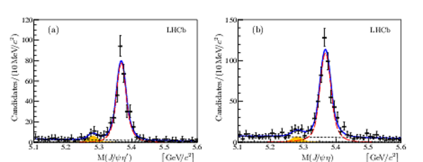
Mass distributions of (a) $ B ^{0}_{(\mathrm{s})} \rightarrow { J \mskip -3mu/\mskip -2mu\psi \mskip 2mu} \eta ^{\prime} $ and (b) $ B ^{0}_{(\mathrm{s})} \rightarrow { J \mskip -3mu/\mskip -2mu\psi \mskip 2mu} \eta $ candidates. The decays $\eta ^{\prime} \rightarrow \eta \pi ^+ \pi ^- $ and $\eta \rightarrow \pi ^+ \pi ^- \pi ^0 $ are used in the reconstruction of $ { J \mskip -3mu/\mskip -2mu\psi \mskip 2mu} \eta ^{\prime} $ and $ { J \mskip -3mu/\mskip -2mu\psi \mskip 2mu} \eta $ candidates, respectively. The total fit function (solid blue) and the combinatorial background contribution (dashed black) are shown. The long-dashed red line represents the signal $ B ^0_ s $ contribution and the yellow shaded area shows the $ B ^0$ contribution.	Fig_2.pdf [94 KiB] HiDef png [183 KiB] Thumbnail [126 KiB] *.C file tex code
Background subtracted $ { J \mskip -3mu/\mskip -2mu\psi \mskip 2mu} \rightarrow \mu ^+\mu ^- $ (a,b), $\eta ^{\prime} \rightarrow \eta \pi ^+ \pi ^- $ (c,d) and $\eta \rightarrow \gamma \gamma $ (e,f) mass distributions in $ B ^{0}_{(\mathrm{s})} \rightarrow { J \mskip -3mu/\mskip -2mu\psi \mskip 2mu} \eta ^{\prime} $ decays. The figures (a,c,e) correspond to $ B ^0_ s $ decays and the figures (b,d,f) correspond to $ B ^0$ decays. The solid curves represent the total fit functions.	Fig_3.pdf [133 KiB] HiDef png [498 KiB] Thumbnail [444 KiB] *.C file tex code
Background subtracted $ { J \mskip -3mu/\mskip -2mu\psi \mskip 2mu} \rightarrow \mu ^+\mu ^- $ (a,b), $\eta \rightarrow \pi ^+ \pi ^- \pi ^0 $ (c,d) and $\pi ^0 \rightarrow \gamma \gamma $ (e,f) mass distributions in $ B ^{0}_{(\mathrm{s})} \rightarrow { J \mskip -3mu/\mskip -2mu\psi \mskip 2mu} \eta $ decays. The figures (a,c,d) correspond to $ B ^0_ s $ decays and the figures (b,d,f) correspond to $ B ^0$ decays. The solid curves represent the total fit functions.	Fig_4.pdf [128 KiB] HiDef png [461 KiB] Thumbnail [405 KiB] *.C file tex code
Mass distributions of (a) $ B ^{0}_{(\mathrm{s})} \rightarrow { J \mskip -3mu/\mskip -2mu\psi \mskip 2mu} \eta ^{\prime} $ and (b) $ B ^{0}_{(\mathrm{s})} \rightarrow \psi {\mathrm{(2S)}} \eta ^{\prime} $ candidates, where the $\eta ^{\prime}$ state is reconstructed using the $\eta ^{\prime} \rightarrow \rho ^0 \gamma $ decay. The total fit function (solid blue) and the combinatorial background contribution (short-dashed black) are shown. The long-dashed red line shows the signal $ B ^0_ s $ contribution and the yellow shaded area corresponds to the $ B ^0$ contribution. The contribution of the reflection from $ B ^0 \rightarrow \psi K ^{*0} $ decays is shown by the green dash-dotted line.	Fig_5.pdf [108 KiB] HiDef png [241 KiB] Thumbnail [178 KiB] *.C file tex code
Background subtracted $\psi \rightarrow \mu ^+\mu ^- $ (a,b) and $\eta ^{\prime} \rightarrow \pi ^+ \pi ^- \gamma $ (c,d) mass distributions in $ B ^0_ s \rightarrow \psi \eta ^{\prime} $ decays. The figures (a,c) correspond to the $ { J \mskip -3mu/\mskip -2mu\psi \mskip 2mu}$ channel, and the figures (b,d) correspond to the $\psi {\mathrm{(2S)}}$ channel. The solid curves represent the total fit functions.	Fig_6.pdf [106 KiB] HiDef png [320 KiB] Thumbnail [288 KiB] *.C file tex code
Confidence regions derived from the likelihood function $\mathcal{L}\left(\varphi_{\rm{P}} ,\left\|\varphi_{\rm{G}} \right\|\right)$. The contours corresponding to $-2\Delta\ln\mathcal{L}=2.3, 6.2$ and $11.8$ are shown with dotted green, dashed blue and solid red lines.	Fig_7.pdf [74 KiB] HiDef png [189 KiB] Thumbnail [163 KiB] *.C file tex code
Animated gif made out of all figures.	PAPER-2014-056.gif Thumbnail

Tables and captions

Mixing angles $\varphi_{\rm{G}} $ and $\varphi_{\rm{P}} $ (in degrees). The third column corresponds to measurements where the gluonic component is neglected. Total uncertainties are quoted.	Table_1.pdf [51 KiB] HiDef png [37 KiB] Thumbnail [18 KiB] tex code
Fit results for the numbers of signal events ($N_{ B ^{0}_{(\mathrm{s})} }$), $ B ^0_ s $ signal peak position ($m_0$) and mass resolution ($\sigma$) in $ B ^{0}_{(\mathrm{s})} \rightarrow { J \mskip -3mu/\mskip -2mu\psi \mskip 2mu} \eta ^{\prime} $ and $ B ^{0}_{(\mathrm{s})} \rightarrow { J \mskip -3mu/\mskip -2mu\psi \mskip 2mu} \eta $ decays, followed by $\eta ^{\prime} \rightarrow \eta \pi ^+ \pi ^- $ and $\eta \rightarrow \pi ^+ \pi ^- \pi ^0 $ decays, respectively. The quoted uncertainties are statistical only.	Table_2.pdf [57 KiB] HiDef png [32 KiB] Thumbnail [16 KiB] tex code
Fitted values of the number of signal events ($N_{ B ^{0}_{(\mathrm{s})} }$), $ B ^0_ s $ signal peak position ($m_0$) and mass resolution ($\sigma$) in $ B ^{0}_{(\mathrm{s})} \rightarrow \psi \eta ^{\prime} $ decays, followed by the $\eta ^{\prime} \rightarrow \rho ^0 \gamma $ decay. The quoted uncertainties are statistical only.	Table_3.pdf [72 KiB] HiDef png [31 KiB] Thumbnail [14 KiB] tex code
Ratios of the total efficiencies as defined in Eqs. 5--7. The quoted uncertainties are statistical only and reflect the sizes of the simulated samples.	Table_4.pdf [51 KiB] HiDef png [88 KiB] Thumbnail [38 KiB] tex code
Systematic uncertainties (in %) of the ratios of the branching fractions.	Table_5.pdf [46 KiB] HiDef png [58 KiB] Thumbnail [28 KiB] tex code