Definition of the angles involved in the analysis of $ B ^0_ s \rightarrow K ^{*0} \overline{ K }{} {}^{*0} $ decays.

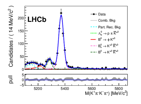
Invariant mass distribution for selected $K^+\pi^- K^- \pi^+$ candidates. The (blue) solid line is the result of the fit explained in the text. The $ B ^0_ s $ and $ B ^0$ signal peaks are shown as as dashed-dotted lines (pink and dark green, respectively). The various peaking background components are represented as dotted lines: (red) $ B ^0 \rightarrow \phi K ^{*0} $ , (green) $\Lambda^0_b \rightarrow p\pi^- K^- \pi^+$ and (light blue) partially reconstructed decays. The (grey) dotted line is the combinatorial background component. The normalised residual (pull) is shown below.

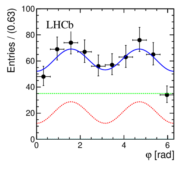
Results of the simultaneous fit to $ B ^0_ s \rightarrow K^+\pi^-K^-\pi^+$ candidates (blue solid line) in the three helicity angles. The dots represent the data after background subtraction and acceptance correction. The red dashed line is the {P--wave} component, the green dashed line is the {S--wave} component and the light-blue dashed line represents the $\mathcal{A}^+_s \mathcal{A}_0$ interference term.

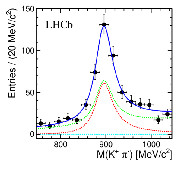
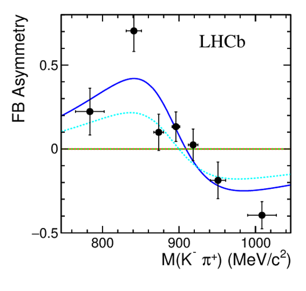
Projections of the model fitted to $ B ^0_ s \rightarrow K^+\pi^-K^-\pi^+$ candidates (blue solid line) in the (top) invariant mass of $K\pi$ pairs and (bottom) $\cos\theta$ asymmetries as functions of $K\pi$ mass ($m_1$, $m_2$). The dots represent the data after background subtraction and acceptance correction. The red dashed line is the {P--wave} component, the green dashed line is the {S--wave} component and the light-blue dashed line represents the ${A}^+_s {A}_0$ interference term.

(Left) Profile likelihood for the parameter $f_L$. (Right) Regions corresponding to $\Delta\ln\mathcal{L} =$ 0.5, 2 and 4.5 (39%, 87% and 99% confidence level) in the $|A_s^-|^2$ -- $f_L$ plane.

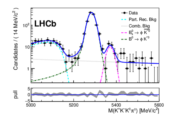
Invariant mass of the selected $K^+K^-K^{\pm}\pi^{\mp}$ combinations and result of the fit to the data. The points represent the data and the (blue) solid line is the fit model. The $ B ^0_ s $ and $ B ^0$ signal peaks are shown as as dashed-dotted lines (pink and dark green, respectively). The contribution from partially reconstructed decays is represented as a (light blue) dashed line. The (grey) dotted line is the combinatorial background component. The normalised residual (pull) is shown below.

Animated gif made out of all figures.

Untagged time-integrated terms used in the analysis, under the assumption of no $ C P$ violation.

Parameters of the mass propagators used in the fit.

Triple product and direct $ C P$ asymmetries measured in this analysis. The first uncertainties are statistical and the second systematic.

Results of the simultaneous fit to $ B ^0_ s \rightarrow K^+\pi^-K^-\pi^+$ TOS and non-TOS candidates with $|M(K^+, \pi^-, K^-, \pi^+) - m_{ B ^0_ s }| < 30 {\mathrm{ Me V /}c^2} $ (phases are measured in radians). The first uncertainties are statistical and the second systematic.

Systematic uncertainties in the measurement of the magnitude and phase of the different amplitudes contributing to the $ B ^0_ s \rightarrow K^+\pi^-K^-\pi^+$ decay.

Summary of relevant quantities in the $ {\cal B}( B ^0_ s \rightarrow K ^{*0} \overline{ K }{} {}^{*0} )$ calculation. The factor $\kappa( B ^0_ s \rightarrow K ^{*0} \overline{ K }{} {}^{*0} )$ is defined as $\lambda_{f_L}( B ^0_ s \rightarrow K ^{*0} \overline{ K }{} {}^{*0} )/f_{ B ^0_ s \rightarrow K ^{*0} \overline{ K }{} {}^{*0} }$, and equivalently for the $ B ^0 \rightarrow \phi K ^{*0} $ decay. The first uncertainty is statistical, the second systematic.