Examples of tree diagrams via $\bar{b} \rightarrow \bar{c}u\bar{d}$ transition to produce (a) $\pi ^+ \pi ^- $ resonances, (b) nonresonant three-body decay and (c) $\overline{ D }{} {}^0 \pi ^- $ resonances.

Invariant mass distribution of $B^0 \rightarrow \overline{ D }{} {}^0 \pi^+\pi^-$ candidates. Data points are shown in black. The fit is shown as a solid (red) line with the background component displayed as dashed (green) line.

Density profile of the combinatorial background events in the Dalitz plane obtained from the upper $m(\overline{ D }{} {}^0 \pi^+\pi^-)$ sideband with a looser selection applied on the Fisher discriminant.

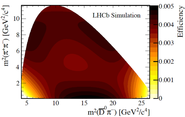
Efficiency function for the Dalitz variables obtained in a fit to the LHCb simulated samples.

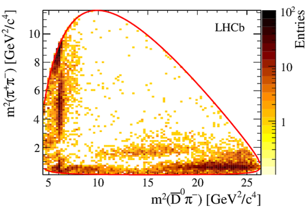
Dalitz plot distribution of candidates in the signal region, including background contributions. The red line shows the Dalitz plot kinematic boundary.

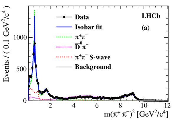
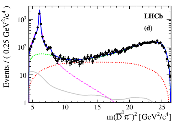
Projections of the data and Isobar fit onto (a) $m^2(\pi^+\pi^-)$ and (c) $m^2(\overline{ D }{} {}^0 \pi^-)$ with a linear scale. Same projections shown in (b) and (d) with a logarithmic scale. Components are described in the legend. The lines denoted $\overline{ D }{} {}^0 \pi^-$ and $\pi^+\pi^-$ include the coherent sums of all $\overline{ D }{} {}^0 \pi^-$ resonances, $\pi^+\pi^-$ resonances, and $\pi^+\pi^-$ S-wave resonances. The various contributions do not add linearly due to interference effects.

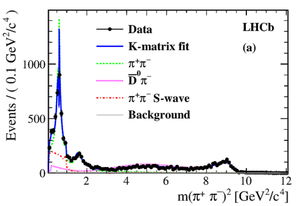
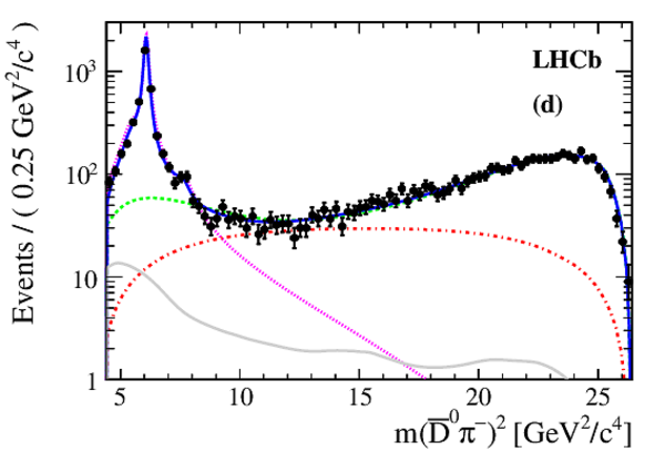
Projections of the data and K-matrix fit onto (a) $m^2(\pi^+\pi^-)$ and (c) $m^2(\overline{ D }{} {}^0 \pi^-)$ with a linear scale. Same projections shown in (b) and (d) with a logarithmic scale. Components are described in the legend. The lines denoted $\overline{ D }{} {}^0 \pi^-$ and $\pi^+\pi^-$ include the coherent sums of all $\overline{ D }{} {}^0 \pi^-$ resonances, $\pi^+\pi^-$ resonances, and $\pi^+\pi^-$ S-wave resonances. The various contributions do not add linearly due to interference effects.

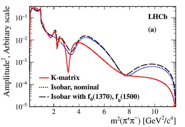
Comparison of the $\pi^+\pi^-$ S-wave obtained from the Isobar model and the K-matrix model, for (a) amplitudes and (b) phases. The K-matrix model is shown by the red solid line, two scenarios for the Isobar model with (black long dashed line) and without (blue dashed line) $f_0(1370)$ and $f_0(1500)$ are shown.

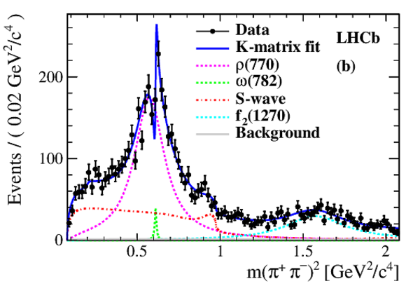
Distributions of $m^2(\pi^+\pi^-)$ in the $\rho(770)$ mass region. The different fit components are described in the legend. Results from (a) the Isobar model and (b) the K-matrix model are shown.

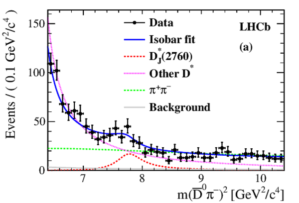
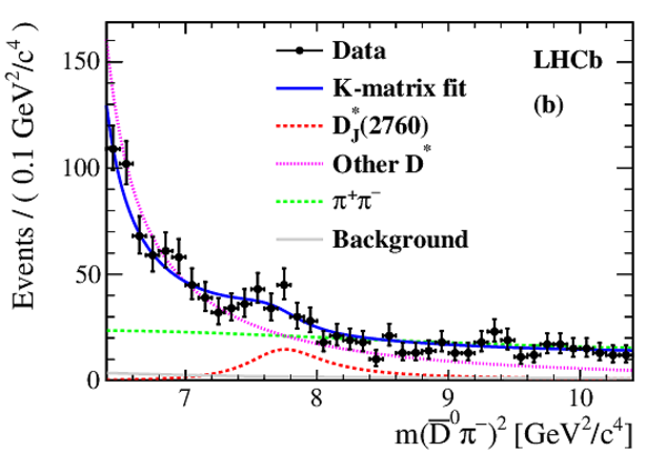
Distributions of $m^2(\overline{ D }{} {}^0 \pi ^- )$ in the $D_J^*(2760)^-$ mass region. The different fit components are described in the legend. Both results from (a) the Isobar model and (b) the K-matrix model are shown.

Invariant mass distributions of (a) $m(\overline{ D }{} {}^0 \pi^+\pi^-)$ and (b) $m(\overline{ D }{} {}^0 \pi^-)$ for $B^0 \rightarrow D^*(2010)^-\pi^+$ candidates. The data is shown as black points with the fit superimposed as red solid lines.

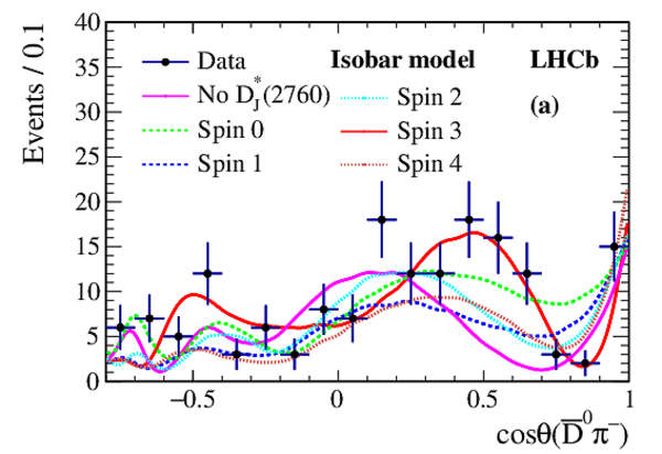
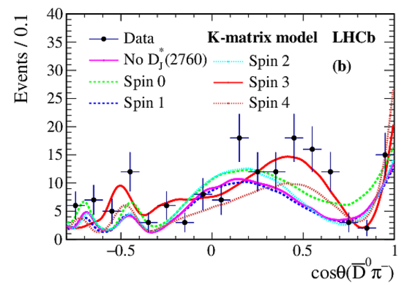
Cosine of the helicity angle distributions in the $m^2(\overline{ D }{} {}^0 \pi^-)$ range [7.4, 8.2] GeV$^2/c^4$ for (a) the Isobar model and (b) the K-matrix model. The data are shown as black points. The helicity angle distributions of the Dalitz plot fit results, without the $D^*_J(2760)^-$ and with the different spin hypotheses of $D^*_J(2760)^-$, are superimposed.

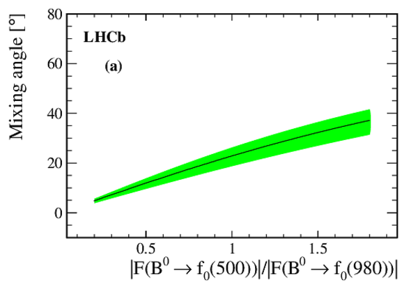
Mixing angle as a function of form factor ratio for the (a) $q\bar{q}$ model and (b) $[qq'][\bar{q}\bar{q'}]$ tetraquark model. Green band gives 1$\sigma$ interval around central values (black solid line).

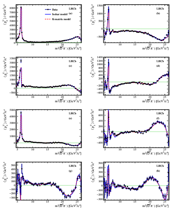
The first eight unnormalised Legendre polynomial weighted moments (0 to 7 correspond to (a) to (h)) for background-subtracted and efficiency-corrected $B^0 \rightarrow \overline{ D }{} {}^0 \pi^+\pi^-$ data and the Dalitz plot fit results as a function of $m^2(\overline{ D }{} {}^0 \pi^-)$.

The first eight unnormalised Legendre polynomial weighted moments (0 to 7 correspond to (a) to (h)) for background-subtracted and efficiency-corrected $B^0 \rightarrow \overline{ D }{} {}^0 \pi^+\pi^-$ data and the Dalitz plot fit results as a function of $m^2(\pi^+\pi^-)$.

The first eight unnormalised Legendre polynomial weighted moments (0 to 7 correspond to (a) to (h)) for background-subtracted and efficiency-corrected $B^0 \rightarrow \overline{ D }{} {}^0 \pi^+\pi^-$ data and the Dalitz plot fit results as a function of $m^2(\overline{ D }{} {}^0 \pi^-)$. Only results in the region $m^2(\overline{ D }{} {}^0 \pi^-)< 10$ GeV$^2$/$c^4$ are shown.

The first eight unnormalised Legendre polynomial weighted moments (0 to 7 correspond to (a) to (h)) for background-subtracted and efficiency-corrected $B^0 \rightarrow \overline{ D }{} {}^0 \pi^+\pi^-$ data and the Dalitz plot fit results as a function of $m^2(\pi^+\pi^-)$. Only results in the region $m^2(\pi^+\pi^-)< 3$ GeV$^2$/$c^4$ are shown.

Animated gif made out of all figures.

Results of the fit to the invariant mass distribution of $B^0 \rightarrow \overline{ D }{} {}^0 \pi^+\pi^-$ candidates. Uncertainties are statistical only.

The K-matrix parameters used in this paper are taken from a global analysis of $\pi^+\pi^-$ scattering data [22]. Masses and coupling constants are in units of $ {\mathrm{ Ge V /}c^2}$ .

Resonant contributions to the nominal fit models and their properties. Parameters and uncertainties of $\rho(770)$, $\omega(782)$, $\rho(1450)$ and $\rho(1700)$ come from Ref. [92], and those of $f_2(1270)$ and $f_0(2020)$ come from Ref. [32]. Parameters of $f_0(500)$, $f_0(980)$ and K-matrix formalism are described in Sec. 4.

Systematic uncertainties on $\cal B ( B ^0 \rightarrow \overline{ D }{} {}^0 \pi ^+ \pi ^- )$.

Statistical significance ($\sigma$) of $\pi^+\pi^-$ resonances in the Dalitz plot analysis. For the statistically significant resonances, the effect of adding dominant systematic uncertainties is shown (see text).

Measured masses ($m$ in $ {\mathrm{ Me V /}c^2}$ ) and widths ($\Gamma$ in $\mathrm{ Me V}$ ) of the $D_0^*(2400)^-$, $D_2^*(2460)^-$ and $D_3^*(2760)^-$ resonances, where the first uncertainty is statistical, the second and the third are experimental and model-dependent systematic uncertainties, respectively.

The moduli of the complex coefficients of the resonant contributions for the Isobar model and the K-matrix model. The first uncertainty is statistical, the second and the third are experimental and model-dependent systematic uncertainties, respectively.

The phase of the complex coefficients of the resonant contributions for the Isobar model and the K-matrix model. The first uncertainty is statistical, the second and the third are experimental and model-dependent systematic uncertainties, respectively.

The fit fractions of the resonant contributions for the Isobar and K-matrix models with $m(\overline{ D }{} {}^0 \pi^{\pm})> 2.1$ $ {\mathrm{ Ge V /}c^2}$ . The first uncertainty is statistical, the second and the third are experimental and model-dependent systematic uncertainties, respectively.

Correction factors due to the $D^*(2010)^-$ veto.

Measured branching fractions of $\cal B ( B ^0 \rightarrow r h_3) \times \cal B (r \rightarrow h_1 h_2)$ for the Isobar and K-matrix models. The first uncertainty is statistical, the second the experimental systematic, the third the model-dependent systematic, and the fourth the uncertainty from the normalisation $B^0 \rightarrow D^*(2010)^- \pi^+$ channel.

Systematic uncertainties on $r^f$. The sum in quadrature of the uncertainties is also reported.

Results of $R_{D\rho}$ and $\cos\delta_{D\rho}$.

Systematic uncertainties on the $\overline{ D }{} {}^0 \pi ^- $ resonant masses (MeV/$c^2$) and widths (MeV) for the Isobar model.

Systematic uncertainties on the moduli of the complex coefficients of the resonant contributions for the Isobar model. The moduli are normalised to that of $\rho(770)$.

Systematic uncertainties on the phases ($^{\circ}$) of the complex coefficients of the resonant contributions for the Isobar model. The phase of $\rho(700)$ is set to $0^{\circ}$ as the reference.

Systematic uncertainties on the fit fractions (%) of the resonant contributions for the Isobar model.

Systematic uncertainties on the $\overline{ D }{} {}^0 \pi ^- $ resonant masses (MeV/$c^2$) and widths (MeV) for the K-matrix model.

Systematic uncertainties on the moduli of the complex coefficients of the resonant contributions for the K-matrix model. The moduli are normalised to that of $\rho(770)$.

Systematic uncertainties on the phases ($^{\circ}$) of the complex coefficients of the resonant contributions for the K-matrix model. The phase of $\rho(700)$ is set to $0^{\circ}$ as reference.

Systematic uncertainties on the fit fractions (%) of the resonant contributions for the K-matrix model.

Interference fit fractions (%) of the resonant contributions for the Isobar model with $m(\overline{ D }{} {}^0 \pi^{\pm})>2.1$ $ {\mathrm{ Ge V /}c^2}$ . The resonances are: ($A_0$) nonresonant S-wave, ($A_1$) $f_0(500)$, ($A_2$) $f_0(980)$, ($A_3$) $f_0(2020)$, ($A_4$) $\rho(770)$, ($A_5$) $\omega(782)$, ($A_6$) $\rho(1450)$, $(A_7)$ $\rho(1700)$, $(A_8)$ $f_2(1270)$, $(A_9)$ $\overline{ D }{} {}^0 \pi^-$ P-wave, $(A_{10})$ $D_0^*(2400)^-$, $(A_{11})$ $D_2^*(2460)^-$, $(A_{12})$ $D_3^*(2760)^-$. The diagonal elements correspond to the fit fractions given in Table 9.

Interference fit fractions (%) of the resonant contributions for the K-matrix model with $m(\overline{ D }{} {}^0 \pi^{\pm})>2.1$ $ {\mathrm{ Ge V /}c^2}$ . The resonances are: ($A_0$) K-matrix S-wave, ($A_1$) $\rho(770)$, ($A_2$) $\omega(782)$, ($A_3$) $\rho(1450)$, $(A_4)$ $\rho(1700)$, $(A_5)$ $f_2(1270)$, $(A_6)$ $\overline{ D }{} {}^0 \pi^-$ P-wave, $(A_{7})$ $D_0^*(2400)^-$, $(A_{8})$ $D_2^*(2460)^-$, $(A_{9})$ $D_3^*(2760)^-$ The diagonal elements correspond to the fit fractions given in Table 9.

Statistical uncertainties on the interference fit fractions (%) of the resonant contributions for the Isobar model with $m(\overline{ D }{} {}^0 \pi^{\pm})>2.1$ $ {\mathrm{ Ge V /}c^2}$ . The resonances are: ($A_0$) nonresonant S-wave, ($A_1$) $f_0(500)$, ($A_2$) $f_0(980)$, ($A_3$) $f_0(2020)$, ($A_4$) $\rho(770)$, ($A_5$) $\omega(782)$, ($A_6$) $\rho(1450)$, $(A_7)$ $\rho(1700)$, $(A_8)$ $f_2(1270)$, $(A_9)$ $\overline{ D }{} {}^0 \pi^-$ P-wave, $(A_{10})$ $D_0^*(2400)^-$, $(A_{11})$ $D_2^*(2460)^-$, $(A_{12})$ $D_3^*(2760)^-$. The diagonal elements correspond to the statistical uncertainties on the fit fractions given in Table 9.

Experimental systematic uncertainties on the interference fit fractions (%) of the resonant contributions for the Isobar model with $m(\overline{ D }{} {}^0 \pi^{\pm})>2.1$ $ {\mathrm{ Ge V /}c^2}$ . The resonances are: ($A_0$) nonresonant S-wave, ($A_1$) $f_0(500)$, ($A_2$) $f_0(980)$, ($A_3$) $f_0(2020)$, ($A_4$) $\rho(770)$, ($A_5$) $\omega(782)$, ($A_6$) $\rho(1450)$, $(A_7)$ $\rho(1700)$, $(A_8)$ $f_2(1270)$, $(A_9)$ $\overline{ D }{} {}^0 \pi^-$ P-wave, $(A_{10})$ $D_0^*(2400)^-$, $(A_{11})$ $D_2^*(2460)^-$, $(A_{12})$ $D_3^*(2760)^-$. The diagonal elements correspond to the statistical uncertainties on the fit fractions given in Table 9.

Model-dependent systematic uncertainties on the interference fit fractions (%) of the resonant contributions for the Isobar model with $m(\overline{ D }{} {}^0 \pi^{\pm})>2.1$ $ {\mathrm{ Ge V /}c^2}$ . The resonances are: ($A_0$) nonresonant S-wave, ($A_1$) $f_0(500)$, ($A_2$) $f_0(980)$, ($A_3$) $f_0(2020)$, ($A_4$) $\rho(770)$, ($A_5$) $\omega(782)$, ($A_6$) $\rho(1450)$, $(A_7)$ $\rho(1700)$, $(A_8)$ $f_2(1270)$, $(A_9)$ $\overline{ D }{} {}^0 \pi^-$ P-wave, $(A_{10})$ $D_0^*(2400)^-$, $(A_{11})$ $D_2^*(2460)^-$, $(A_{12})$ $D_3^*(2760)^-$. The diagonal elements correspond to the statistical uncertainties on the fit fractions given in Table 9.

Statistical uncertainties on the interference fit fractions (%) of the resonant contributions for the K-matrix model with $m(\overline{ D }{} {}^0 \pi^{\pm})>2.1$ $ {\mathrm{ Ge V /}c^2}$ . The resonances are: ($A_0$)K-matrix S-wave, ($A_1$) $\rho(770)$, ($A_2$) $\omega(782)$, ($A_3$) $\rho(1450)$, $(A_4)$ $\rho(1700)$, $(A_5)$ $f_2(1270)$, $(A_6)$ $\overline{ D }{} {}^0 \pi^-$ P-wave, $(A_{7})$ $D_0^*(2400)^-$, $(A_{8})$ $D_2^*(2460)^-$, $(A_{9})$ $D_3^*(2760)^-$ The diagonal elements correspond to the statistical uncertainties on the fit fractions shown in Table 9.

Experimental systematic uncertainties on the interference fit fractions (%) of the resonant contributions for the K-matrix model with $m(\overline{ D }{} {}^0 \pi^{\pm})>2.1$ $ {\mathrm{ Ge V /}c^2}$ . The resonances are: ($A_0$) K-matrix S-wave, ($A_1$) $\rho(770)$, ($A_2$) $\omega(782)$, ($A_3$) $\rho(1450)$, $(A_4)$ $\rho(1700)$, $(A_5)$ $f_2(1270)$, $(A_6)$ $\overline{ D }{} {}^0 \pi^-$ P-wave, $(A_{7})$ $D_0^*(2400)^-$, $(A_{8})$ $D_2^*(2460)^-$, $(A_{9})$ $D_3^*(2760)^-$ The diagonal elements correspond to the statistical uncertainties on the fit fractions shown in Table 9.

Model-dependent systematic uncertainties on the interference fit fractions (%) of the resonant contributions for the K-matrix model with $m(\overline{ D }{} {}^0 \pi^{\pm})>2.1$ $ {\mathrm{ Ge V /}c^2}$ . The resonances are: ($A_0$) K-matrix S-wave, ($A_1$) $\rho(770)$, ($A_2$) $\omega(782)$, ($A_3$) $\rho(1450)$, $(A_4)$ $\rho(1700)$, $(A_5)$ $f_2(1270)$, $(A_6)$ $\overline{ D }{} {}^0 \pi^-$ P-wave, $(A_{7})$ $D_0^*(2400)^-$, $(A_{8})$ $D_2^*(2460)^-$, $(A_{9})$ $D_3^*(2760)^-$ The diagonal elements correspond to the statistical uncertainties on the fit fractions shown in Table 9.

The moduli and phases of the K-matrix parameters. The first uncertainty is statistical, the second the experimental systematic, and the third the model-dependent systematic. The moduli are normalised to that of the $\rho(770)$ contribution and the phase of $\rho(770)$ is set to 0$^{\circ}$.

Systematic uncertainties on the moduli of the K-matrix parameters. The moduli are normalised to that of $\rho(770)$.

Systematic uncertainties on the phases ($^{\circ}$) of the K-matrix parameters. The phase of $\rho(700)$ is set to 0$^{\circ}$ as the reference.