First observation and amplitude analysis of the $B^{-}\to D^{+}K^{-}\pi^{-}$ decay

Information

LHCb-PAPER-2015-007
CERN-PH-EP-2015-051
arXiv:1503.02995 [PDF]

(Submitted on 10 Mar 2015)
Phys. Rev. D91 (2015) 092002
Inspire 1351449

Tools

Abstract

The $B^{-}\to D^{+}K^{-}\pi^{-}$ decay is observed in a data sample corresponding to $3.0 \rm{fb}^{-1}$ of $pp$ collision data recorded by the LHCb experiment during 2011 and 2012. Its branching fraction is measured to be ${\cal B}(B^{-}\to D^{+}K^{-}\pi^{-}) = (7.31 \pm 0.19 \pm 0.22 \pm 0.39) \times 10^{-5}$ where the uncertainties are statistical, systematic and from the branching fraction of the normalisation channel $B^{-}\to D^{+}\pi^{-}\pi^{-}$, respectively. An amplitude analysis of the resonant structure of the $B^{-}\to D^{+}K^{-}\pi^{-}$ decay is used to measure the contributions from quasi-two-body $B^{-}\to D_{0}^{*}(2400)^{0}K^{-}$, $B^{-}\to D_{2}^{*}(2460)^{0}K^{-}$, and $B^{-}\to D_{J}^{*}(2760)^{0}K^{-}$ decays, as well as from nonresonant sources. The $D_{J}^{*}(2760)^{0}$ resonance is determined to have spin 1.

Figures and captions

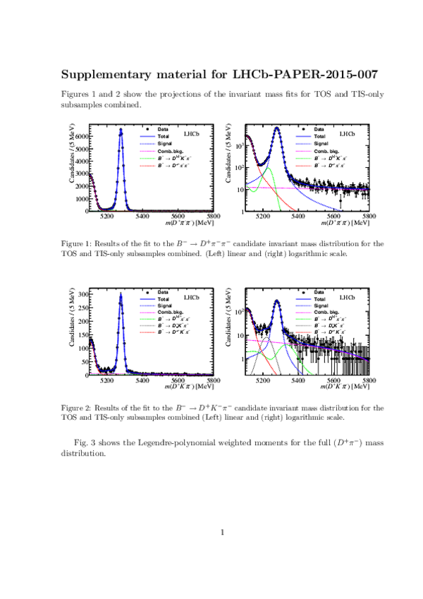
Results of the fit to the $ B ^- \rightarrow D ^+ \pi ^- \pi ^- $ candidate invariant mass distribution for the (left) TOS and (right) TIS-only subsamples. Data points are shown in black, the full fitted model as solid blue lines and the components as shown in the legend.	Fig1a.pdf [31 KiB] HiDef png [290 KiB] Thumbnail [250 KiB] *.C file
	Fig1b.pdf [30 KiB] HiDef png [295 KiB] Thumbnail [256 KiB] *.C file
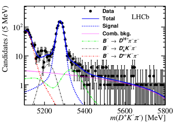
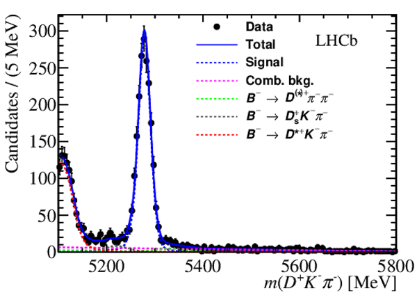
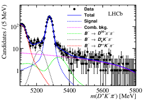
Results of the fit to the $ B ^- \rightarrow D ^+ K ^- \pi ^- $ candidate invariant mass distribution for the (left) TOS and (right) TIS-only subsamples. Data points are shown in black, the full fitted model as solid blue lines and the components as shown in the legend.	Fig2a.pdf [29 KiB] HiDef png [325 KiB] Thumbnail [279 KiB] *.C file
	Fig2b.pdf [29 KiB] HiDef png [316 KiB] Thumbnail [276 KiB] *.C file
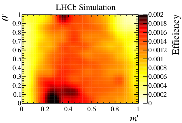
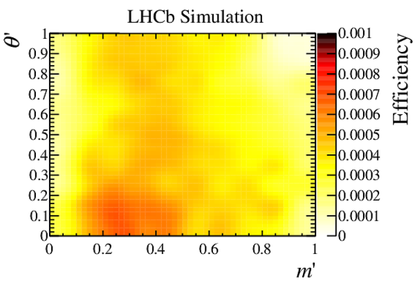
Signal efficiency across the SDP for (left) TOS and (right) TIS-only $ B ^- \rightarrow D ^+ K ^- \pi ^- $ decays. The relative uncertainty at each point is typically $5 \%$.	Fig3a.pdf [32 KiB] HiDef png [422 KiB] Thumbnail [387 KiB] *.C file
	Fig3b.pdf [31 KiB] HiDef png [409 KiB] Thumbnail [363 KiB] *.C file
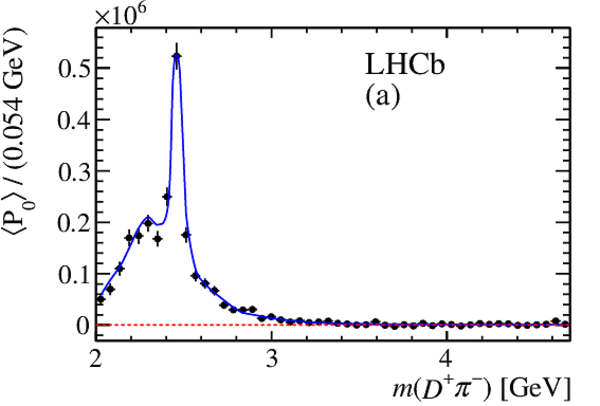
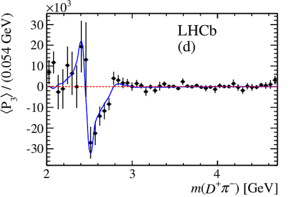
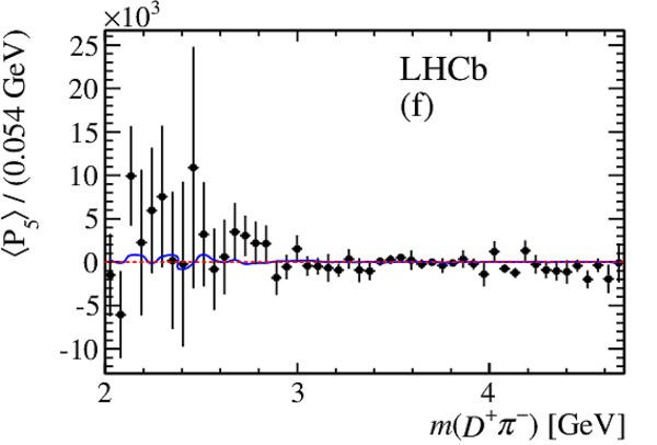
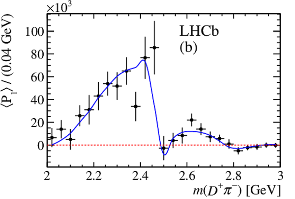
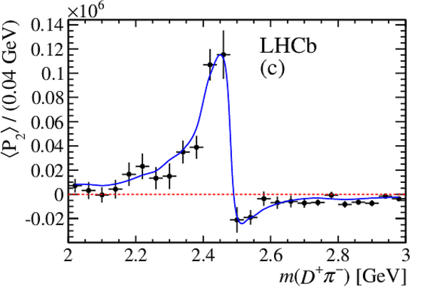
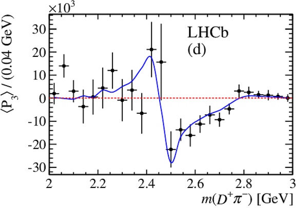
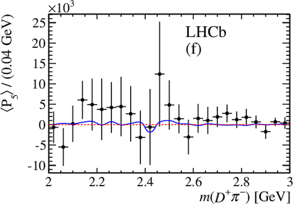
The first seven Legendre-polynomial weighted moments for background-subtracted and efficiency-corrected $ B ^- \rightarrow D ^+ K ^- \pi ^- $ data (black points) as a function of $m( D ^+ \pi ^- )$ in the range $2.0$--$3.0\mathrm{ Ge V} $. Candidates from both TOS and TIS-only subsamples are included. The blue line shows the result of the DP fit described in Sec. 7.	Fig4a.pdf [17 KiB] HiDef png [156 KiB] Thumbnail [133 KiB] *.C file
	Fig4b.pdf [17 KiB] HiDef png [176 KiB] Thumbnail [155 KiB] *.C file
	Fig4c.pdf [17 KiB] HiDef png [180 KiB] Thumbnail [164 KiB] *.C file
	Fig4d.pdf [18 KiB] HiDef png [169 KiB] Thumbnail [149 KiB] *.C file
	Fig4e.pdf [17 KiB] HiDef png [165 KiB] Thumbnail [142 KiB] *.C file
	Fig4f.pdf [19 KiB] HiDef png [154 KiB] Thumbnail [147 KiB] *.C file
	Fig4g.pdf [19 KiB] HiDef png [153 KiB] Thumbnail [144 KiB] *.C file
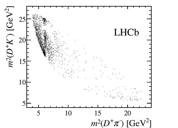
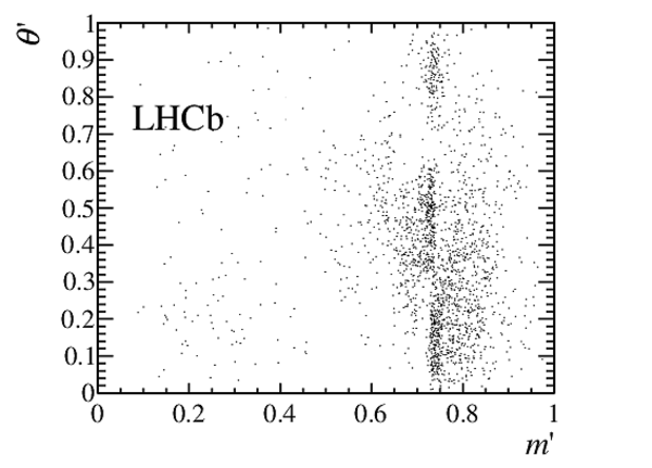
Distribution of $ B ^- \rightarrow D ^+ K ^- \pi ^- $ candidates in the signal region over (left) the DP and (right) the SDP. Candidates from both TOS and TIS-only subsamples are included.	Fig5a.pdf [34 KiB] HiDef png [116 KiB] Thumbnail [59 KiB] *.C file
	Fig5b.pdf [35 KiB] HiDef png [143 KiB] Thumbnail [86 KiB] *.C file
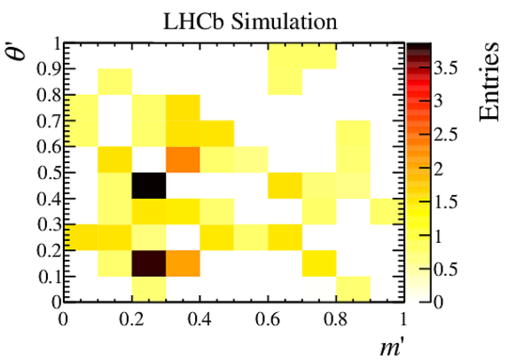
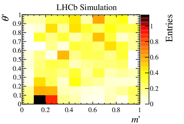
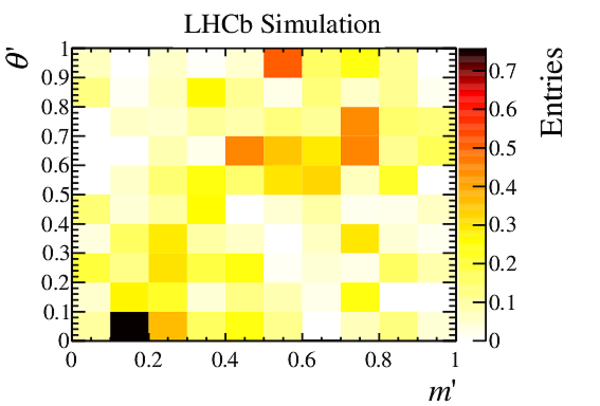
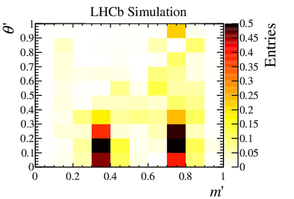
Square Dalitz plot distributions used in the Dalitz plot fit for (top) combinatorial background, (middle) $ B ^- \rightarrow D^{(*)+}\pi ^- \pi ^- $ decays and (bottom) $ B ^- \rightarrow D ^+_ s K ^- \pi ^- $ decays. Candidates the TOS (TIS-only) subsamples are shown in the left (right) column.	Fig6a.pdf [17 KiB] HiDef png [144 KiB] Thumbnail [138 KiB] *.C file
	Fig6b.pdf [17 KiB] HiDef png [141 KiB] Thumbnail [135 KiB] *.C file
	Fig6c.pdf [17 KiB] HiDef png [166 KiB] Thumbnail [146 KiB] *.C file
	Fig6d.pdf [17 KiB] HiDef png [168 KiB] Thumbnail [150 KiB] *.C file
	Fig6e.pdf [17 KiB] HiDef png [166 KiB] Thumbnail [151 KiB] *.C file
	Fig6f.pdf [17 KiB] HiDef png [171 KiB] Thumbnail [157 KiB] *.C file
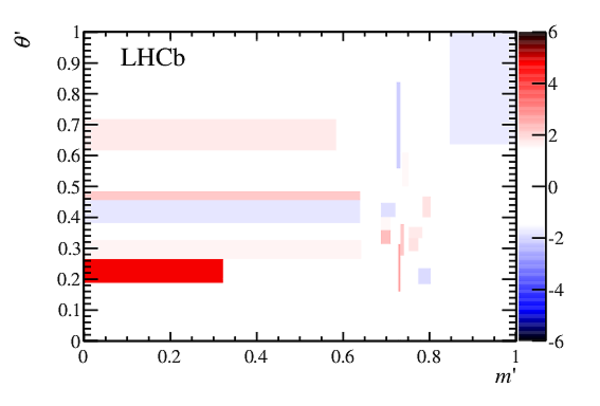
Differences between the data SDP distribution and the fit model across the SDP, in terms of the per-bin pull.	Fig7.pdf [18 KiB] HiDef png [114 KiB] Thumbnail [103 KiB] *.C file
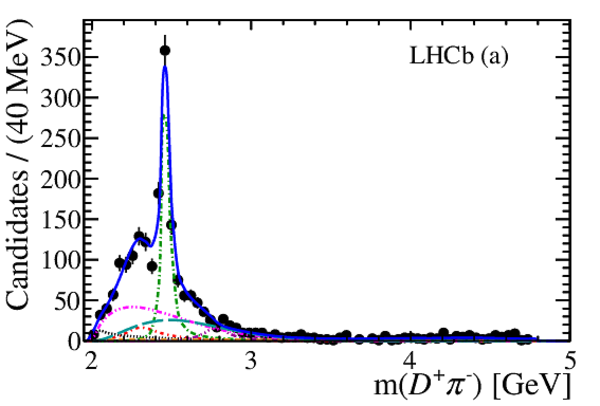
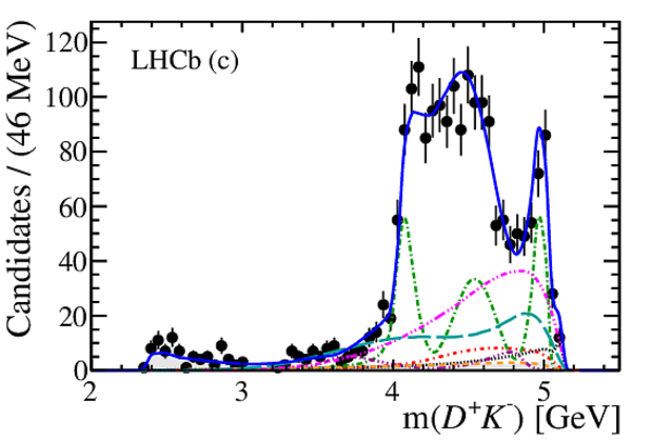
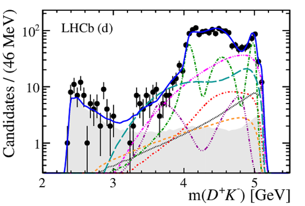
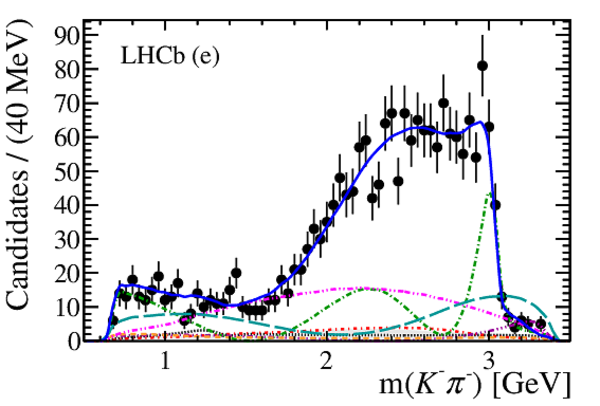
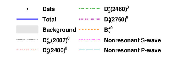
Projections of the data and amplitude fit onto (a) $m(D\pi)$, (c) $m(DK)$ and (e) $m(K\pi)$, with the same projections shown in (b), (d) and (f) with a logarithmic $y$-axis scale. Components are described in the legend.	Fig8a.pdf [27 KiB] HiDef png [219 KiB] Thumbnail [171 KiB] *.C file
	Fig8b.pdf [25 KiB] HiDef png [376 KiB] Thumbnail [266 KiB] *.C file
	Fig8c.pdf [26 KiB] HiDef png [287 KiB] Thumbnail [204 KiB] *.C file
	Fig8d.pdf [25 KiB] HiDef png [411 KiB] Thumbnail [274 KiB] *.C file
	Fig8e.pdf [29 KiB] HiDef png [322 KiB] Thumbnail [238 KiB] *.C file
	Fig8f.pdf [28 KiB] HiDef png [380 KiB] Thumbnail [272 KiB] *.C file
	Fig8g.pdf [12 KiB] HiDef png [96 KiB] Thumbnail [94 KiB] *.C file
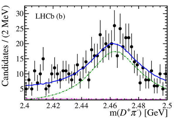
Projections of the data and amplitude fit onto $m(D\pi)$ in (a) the threshold region, (b) the $D^_2(2460)^0$ region and (c) the $D^_1(2760)^0$ region. Components are as shown in Fig. 8.	Fig9a.pdf [24 KiB] HiDef png [248 KiB] Thumbnail [206 KiB] *.C file
	Fig9b.pdf [19 KiB] HiDef png [224 KiB] Thumbnail [197 KiB] *.C file
	Fig9c.pdf [30 KiB] HiDef png [280 KiB] Thumbnail [208 KiB] *.C file
Projections of the data and amplitude fit onto the cosine of the helicity angle for the $D\pi$ system in (a) the threshold region, (b) the $D^_2(2460)^0$ region and (c) the $D^_1(2760)^0$ region. Components are as shown in Fig. 8.	Fig10a.pdf [25 KiB] HiDef png [259 KiB] Thumbnail [203 KiB] *.C file
	Fig10b.pdf [25 KiB] HiDef png [243 KiB] Thumbnail [191 KiB] *.C file
	Fig10c.pdf [27 KiB] HiDef png [296 KiB] Thumbnail [212 KiB] *.C file
Animated gif made out of all figures.	PAPER-2015-007.gif Thumbnail

Tables and captions

Measured properties of neutral $D^{**}$ states. Where more than one uncertainty is given, the first is statistical and the others systematic.	Table_1.pdf [53 KiB] HiDef png [92 KiB] Thumbnail [45 KiB] tex code
Yields of the various components in the fit to $ B ^- \rightarrow D ^+ \pi ^- \pi ^- $ candidate invariant mass distribution.	Table_2.pdf [46 KiB] HiDef png [53 KiB] Thumbnail [27 KiB] tex code
Yields of the various components in the fit to $ B ^- \rightarrow D ^+ K ^- \pi ^- $ candidate invariant mass distribution.	Table_3.pdf [53 KiB] HiDef png [72 KiB] Thumbnail [35 KiB] tex code
Relative systematic uncertainties on the measurement of the ratio of branching fractions for $ B ^- \rightarrow D ^+ K ^- \pi ^- $ and $ B ^- \rightarrow D ^+ \pi ^- \pi ^- $ decays.	Table_4.pdf [30 KiB] HiDef png [60 KiB] Thumbnail [27 KiB] tex code
Signal contributions to the fit model, where parameters and uncertainties are taken from Ref. [9]. States labelled with subscript $v$ are virtual contributions.	Table_5.pdf [56 KiB] HiDef png [78 KiB] Thumbnail [34 KiB] tex code
Masses and widths determined in the fit to data, with statistical uncertainties only.	Table_6.pdf [50 KiB] HiDef png [51 KiB] Thumbnail [23 KiB] tex code
Complex coefficients and fit fractions determined from the Dalitz plot fit. Uncertainties are statistical only.	Table_7.pdf [55 KiB] HiDef png [79 KiB] Thumbnail [34 KiB] tex code
Experimental systematic uncertainties on the fit fractions and complex amplitudes.	Table_8.pdf [47 KiB] HiDef png [56 KiB] Thumbnail [23 KiB] tex code
Model uncertainties on the fit fractions and complex amplitudes.	Table_9.pdf [47 KiB] HiDef png [55 KiB] Thumbnail [24 KiB] tex code
Breakdown of experimental systematic uncertainties on the fit fractions (%) and masses $(\mathrm{Me V} )$ and widths $(\mathrm{Me V} )$.	Table_10.pdf [61 KiB] HiDef png [94 KiB] Thumbnail [44 KiB] tex code
Breakdown of model uncertainties on the fit fractions (%) and masses $(\mathrm{Me V} )$ and widths $(\mathrm{Me V} )$.	Table_11.pdf [61 KiB] HiDef png [80 KiB] Thumbnail [37 KiB] tex code
Results for the complex amplitudes and their uncertainties. The three quoted errors are statistical, experimental systematic and model uncertainties, respectively.	Table_12.pdf [53 KiB] HiDef png [83 KiB] Thumbnail [41 KiB] tex code
Results for the complex amplitudes and their uncertainties. The three quoted errors are statistical, experimental systematic and model uncertainties, respectively.	Table_13.pdf [53 KiB] HiDef png [86 KiB] Thumbnail [40 KiB] tex code
Results for the fit fractions and their uncertainties (%). The three quoted errors are statistical, experimental systematic and model uncertainties, respectively.	Table_14.pdf [51 KiB] HiDef png [103 KiB] Thumbnail [51 KiB] tex code
Results for the product branching fractions ${\cal B}( B ^- \rightarrow R K ^- ) \times {\cal B}(R \rightarrow D ^+ \pi ^- )$ ($10^{-6}$). The four quoted errors are statistical, experimental systematic, model and inclusive branching fraction uncertainties, respectively.	Table_15.pdf [52 KiB] HiDef png [97 KiB] Thumbnail [51 KiB] tex code
Results for the fit fractions and complex coefficients for the secondary minima with $2{\rm NLL}$ values 2.8 and 3.3 units greater than that of the global minimum of the NLL function.	Table_16.pdf [56 KiB] HiDef png [67 KiB] Thumbnail [28 KiB] tex code
Interference fit fractions (%) and statistical uncertainties. The amplitudes are: ($A_0$) $D^_v(2007)^0$, ($A_1$) $D^_0(2400)^0$, ($A_2$) $D^_2(2460)^0$, ($A_3$) $D^_1(2760)^0$, ($A_4$) $B^*_v$, ($A_5$) nonresonant S-wave, ($A_6$) nonresonant P-wave. The diagonal elements are the same as the conventional fit fractions.	Table_17.pdf [33 KiB] HiDef png [41 KiB] Thumbnail [19 KiB] tex code
Experimental systematic uncertainies on the interference fit fractions (%). The amplitudes are: ($A_0$) $D^_v(2007)^0$, ($A_1$) $D^_0(2400)^0$, ($A_2$) $D^_2(2460)^0$, ($A_3$) $D^_1(2760)^0$, ($A_4$) $B^*_v$, ($A_5$) nonresonant S-wave, ($A_6$) nonresonant P-wave. The diagonal elements are the same as the conventional fit fractions.	Table_18.pdf [27 KiB] HiDef png [68 KiB] Thumbnail [31 KiB] tex code
Model systematic uncertainies on the interference fit fractions (%). The amplitudes are: ($A_0$) $D^_v(2007)^0$, ($A_1$) $D^_0(2400)^0$, ($A_2$) $D^_2(2460)^0$, ($A_3$) $D^_1(2760)^0$, ($A_4$) $B^*_v$, ($A_5$) nonresonant S-wave, ($A_6$) nonresonant P-wave. The diagonal elements are the same as the conventional fit fractions.	Table_19.pdf [27 KiB] HiDef png [43 KiB] Thumbnail [17 KiB] tex code

Supplementary Material [file]

Supplementary material full pdf	supple[..].pdf [292 KiB]
	Fig11a.pdf [31 KiB] HiDef png [243 KiB] Thumbnail [206 KiB] *C file
	Fig11b.pdf [31 KiB] HiDef png [277 KiB] Thumbnail [240 KiB] *C file
	Fig12a.pdf [31 KiB] HiDef png [265 KiB] Thumbnail [213 KiB] *C file
	Fig12b.pdf [30 KiB] HiDef png [315 KiB] Thumbnail [282 KiB] *C file
	Fig13a.pdf [16 KiB] HiDef png [185 KiB] Thumbnail [175 KiB] *C file
	Fig13b.pdf [16 KiB] HiDef png [165 KiB] Thumbnail [151 KiB] *C file
	Fig13c.pdf [16 KiB] HiDef png [182 KiB] Thumbnail [174 KiB] *C file
	Fig13d.pdf [16 KiB] HiDef png [172 KiB] Thumbnail [159 KiB] *C file
	Fig13e.pdf [16 KiB] HiDef png [165 KiB] Thumbnail [149 KiB] *C file
	Fig13f.pdf [17 KiB] HiDef png [158 KiB] Thumbnail [155 KiB] *C file
	Fig13g.pdf [17 KiB] HiDef png [155 KiB] Thumbnail [148 KiB] *C file