Observation of the decay $\overline{B}_s^0 \rightarrow \psi(2S) K^+ \pi^-$
[to restricted-access page]Information
LHCb-PAPER-2015-010
CERN-PH-EP-2015-072
arXiv:1503.07112 [PDF]
(Submitted on 24 Mar 2015)
Phys. Lett. B747 (2015) 484
Inspire 1355376
Tools
Abstract
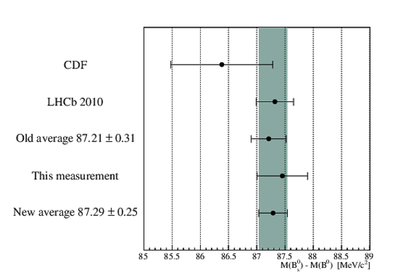
The decay $\overline{B}_s^0 \rightarrow \psi(2S) K^+ \pi^-$ is observed using a data set corresponding to an integrated luminosity of $3.0fb^{-1}$ collected by the LHCb experiment in $pp$ collisions at centre-of-mass energies of 7 and 8 TeV. The branching fraction relative to the $B^0\rightarrow \psi(2S) K^+ \pi^-$ decay mode is measured to be \begin{equation} \frac{{\cal B}(\overline{B}^0_s \rightarrow \psi(2S) K^+ \pi^-)}{{\cal B}(B^0 \rightarrow \psi(2S) K^+ \pi^-)} = 5.38 \pm 0.36 (stat) \pm 0.22 (syst) \pm 0.31 (f_s/f_d) \%,\nonumber \end{equation} where $f_s/f_d$ indicates the uncertainty due to the ratio of probabilities for a $b$ quark to hadronise into a $B_s^0$ or $B^0$ meson. Using an amplitude analysis, the fraction of decays proceeding via an intermediate $K^*(892)^0$ meson is measured to be $0.645 \pm 0.049 (stat) \pm 0.049 (syst)$ and its longitudinal polarisation fraction is $0.524 \pm 0.056 (stat) \pm 0.029 (syst)$. The relative branching fraction for this component is determined to be \begin{equation} \frac{{\cal B}(\overline{B}^0_s \rightarrow \psi(2S) K^*(892)^0)}{{\cal B}(B^0 \rightarrow \psi(2S) K^*(892)^0)} = 5.58 \pm 0.57 (stat) \pm 0.40 (syst) \pm 0.32 (f_s/f_d) \%. \nonumber \end{equation} In addition, the mass splitting between the $B_s^0$ and $B^0$ mesons is measured as \begin{equation} M(B^0_s) - M(B^0) = 87.45 \pm 0.44 (stat) \pm 0.07 (syst) MeV/c^2. \nonumber \end{equation}
Figures and captions
|
Tree (left) and penguin (right) topologies contributing to the $ B ^0_{( s )} \rightarrow \psi V$ decays where $\psi = J/\psi, \psi(2S)$ and $V = \phi, K^*(892)^0$. |
Fig1a.pdf [9 KiB] HiDef png [115 KiB] Thumbnail [63 KiB] *.C file |

|
|
Fig1b.pdf [10 KiB] HiDef png [148 KiB] Thumbnail [83 KiB] *.C file |

|
|
|
Invariant mass distribution for selected $\psi(2S)K^+ \pi^-$ candidates in the data. A fit to the model described in the text is superimposed. The full fit model is shown by the solid (red) line, the combinatorial background by the solid (yellow) and the sum of background from the exclusive $b \rightarrow \psi(2S)X$ modes considered in the text by the shaded (blue) area. The maximum of the $y$-scale is restricted so as to be able to see more clearly the $\overline{ B }{} {}^0_ s \rightarrow \psi(2S)K^+ \pi^-$ signal. The lower plot shows the differences between the fit and measured values divided by the corresponding uncertainty of the measured value, the so-called pull distribution. |
Fig2.pdf [16 KiB] HiDef png [244 KiB] Thumbnail [186 KiB] *.C file |

|
|
Dalitz plot for the selected $\overline{ B }{} {}^0_ s \rightarrow \psi(2S) K ^+ \pi^-$ candidates in the signal window $m(\psi(2S) K ^+ \pi^-) \in [5350, 5380] {\mathrm{ Me V /}c^2} $. |
Fig3.pdf [27 KiB] HiDef png [166 KiB] Thumbnail [100 KiB] *.C file |

|
|
Definition of the helicity angles. |
Fig4.png [85 KiB] HiDef png [23 KiB] Thumbnail [8 KiB] *.C file |

|
|
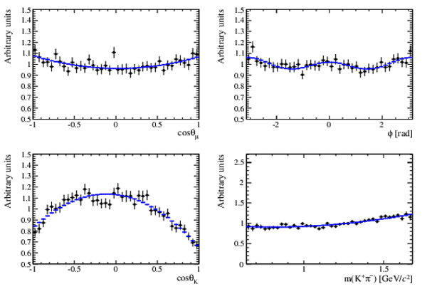
Distributions of (a) $\cos\theta_\mu$, (b) $\phi$, (c) $\cos\theta_K$ and (d) $m( K ^+ \pi^-)$ of simulated $B^0_s\rightarrow \psi(2S) K ^+ \pi^-$ decays in a phase space configuration (black points) with the parameterisation of the efficiency overlaid (blue lines). |
Fig5.pdf [38 KiB] HiDef png [240 KiB] Thumbnail [213 KiB] *.C file |
|
|
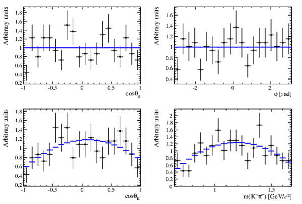
Distributions of (a) $\cos\theta_\mu$, (b) $\phi$, (c) $\cos\theta_K$ and (d) $m( K ^+ \pi^-)$ of $B^0_{(s)}\rightarrow \psi(2S) K ^+ \pi^-$ candidates with $m(\psi(2S) K ^+ \pi^-) > 5390 {\mathrm{ Me V /}c^2} $ (black points), with the parameterisation of the background distribution overlaid (blue lines). |
Fig6.pdf [26 KiB] HiDef png [207 KiB] Thumbnail [209 KiB] *.C file |
|
|
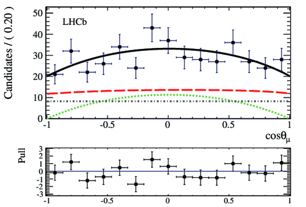
Distributions of (a) $\cos\theta_\mu$, (b) $\phi$, (c) $\cos\theta_K$ and (d) $m( K ^+ \pi^-)$ for selected $\overline{ B }{} {}^0_ s \rightarrow \psi(2S) K ^+ \pi^-$ candidates (black points) with the projections of the fitted amplitude model overlaid. The following components are included in the model: $K^*(892)^0$ (red dashed), LASS S-wave (green dotted), and background (grey dashed-dotted). The residual pulls are shown below each distribution. |
Fig7a.pdf [21 KiB] HiDef png [469 KiB] Thumbnail [183 KiB] *.C file |
|
|
Fig7b.pdf [20 KiB] HiDef png [425 KiB] Thumbnail [160 KiB] *.C file |

|
|
|
Fig7c.pdf [20 KiB] HiDef png [451 KiB] Thumbnail [173 KiB] *.C file |

|
|
|
Fig7d.pdf [23 KiB] HiDef png [496 KiB] Thumbnail [184 KiB] *.C file |

|
|
|
Animated gif made out of all figures. |
PAPER-2015-010.gif Thumbnail |

|
![HiDef png [115 KiB]](Directory_LHCb-PAPER-2015-010/hidef_Fig1a.png)
![HiDef png [148 KiB]](Directory_LHCb-PAPER-2015-010/hidef_Fig1b.png)
![HiDef png [244 KiB]](Directory_LHCb-PAPER-2015-010/hidef_Fig2.png)
![HiDef png [166 KiB]](Directory_LHCb-PAPER-2015-010/hidef_Fig3.png)
![Fig4.png [85 KiB]](Directory_LHCb-PAPER-2015-010/Fig4.png)
![HiDef png [23 KiB]](Directory_LHCb-PAPER-2015-010/hidef_Fig4.png)
![HiDef png [240 KiB]](Directory_LHCb-PAPER-2015-010/hidef_Fig5.png)
![HiDef png [207 KiB]](Directory_LHCb-PAPER-2015-010/hidef_Fig6.png)
![HiDef png [469 KiB]](Directory_LHCb-PAPER-2015-010/hidef_Fig7a.png)
![HiDef png [425 KiB]](Directory_LHCb-PAPER-2015-010/hidef_Fig7b.png)
![HiDef png [451 KiB]](Directory_LHCb-PAPER-2015-010/hidef_Fig7c.png)
![HiDef png [496 KiB]](Directory_LHCb-PAPER-2015-010/hidef_Fig7d.png)
Tables and captions
|
Summary of systematic uncertainties on the $K^*(892)^0$ fit fraction and $f_{\rm L}$. Rows marked with (*) refer to uncorrelated sources of uncertainty between the $ B ^0_ s $ and $ B ^0 $ modes for the computation of the ratio of branching fractions. |
Table_1.pdf [50 KiB] HiDef png [97 KiB] Thumbnail [39 KiB] tex code |

|
|
Systematic uncertainties on the ratio of branching fractions. |
Table_2.pdf [38 KiB] HiDef png [79 KiB] Thumbnail [35 KiB] tex code |

|
![HiDef png [97 KiB]](Directory_LHCb-PAPER-2015-010/hidef_Table_1.png)
![HiDef png [79 KiB]](Directory_LHCb-PAPER-2015-010/hidef_Table_2.png)
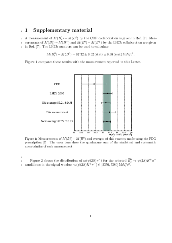
Supplementary Material [file]
| Supplementary material full pdf |
supple[..].pdf [123 KiB] |
|
|
Fig8.pdf [3 KiB] HiDef png [175 KiB] Thumbnail [144 KiB] *C file |
|
|
|
Fig9.pdf [14 KiB] HiDef png [142 KiB] Thumbnail [132 KiB] *C file |

|
![HiDef png [175 KiB]](Directory_LHCb-PAPER-2015-010/supplementary/hidef_Fig8.png)
![HiDef png [142 KiB]](Directory_LHCb-PAPER-2015-010/supplementary/hidef_Fig9.png)
Created on 27 April 2024.