An angular analysis and a measurement of the differential branching fraction
of the decay $B^0_s\to\phi\mu^+\mu^-$ are presented, using data corresponding
to an integrated luminosity of $3.0 {\rm fb^{-1}}$ of $pp$ collisions
recorded by the LHCb experiment at $\sqrt{s} = 7$ and $8 {\rm TeV}$.
Measurements are reported as a function of $q^{2}$, the square of the dimuon
invariant mass and results of the angular analysis are found to be consistent
with the Standard Model. In the range $1<q^2<6 {\rm GeV}^{2}/c^{4}$, where
precise theoretical calculations are available, the differential branching
fraction is found to be more than $3 \sigma$ below the Standard Model
predictions.
|
Examples of $b\rightarrow s$ loop diagrams contributing to the decay $ B ^0_ s \rightarrow \phi\mu ^+\mu ^- $ in the SM.
|
Fig_1.pdf [40 KiB]
HiDef png [15 KiB]
Thumbnail [8 KiB]
*.C file
tex code
|

|
|
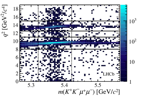
Two-dimensional distribution of $ q^2$ versus the invariant mass of the $ K ^+ K ^- \mu ^+\mu ^- $ system.
The signal decay $ B ^0_ s \rightarrow \phi\mu ^+\mu ^- $ is clearly visible within the $\pm50 {\mathrm{ Me V /}c^2} $ interval around the $ B ^0_ s $ mass, indicated by the dashed vertical lines.
The horizontal lines denote the charmonium regions, where the tree-level decays $ B ^0_ s \rightarrow { J \mskip -3mu/\mskip -2mu\psi \mskip 2mu} \phi $ and $ B ^0_ s \rightarrow \psi {(2S)} \phi $ dominate.
|
mbvsq2.pdf [15 KiB]
HiDef png [399 KiB]
Thumbnail [424 KiB]
*.C file
|
|
|
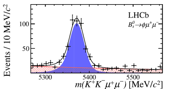
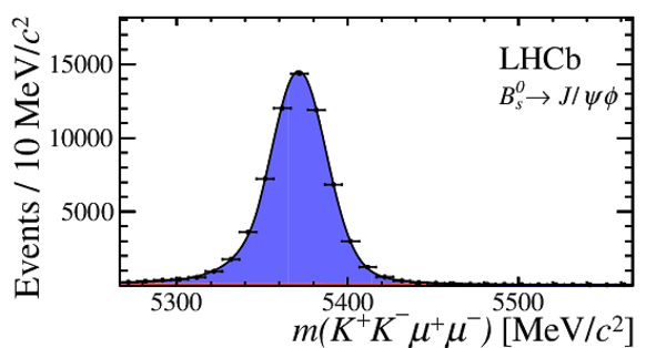
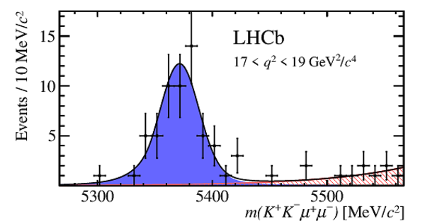
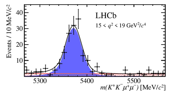
Invariant mass distribution for (left) $ B ^0_ s \rightarrow \phi\mu ^+\mu ^- $ signal decays,
integrated over the $q^2$ bins used,
and for (right) the control mode $ B ^0_ s \rightarrow { J \mskip -3mu/\mskip -2mu\psi \mskip 2mu} \phi $ in the $ K ^+ K ^- \mu ^+\mu ^- $ final state.
The signal component is given by the solid blue area, the background component by the shaded red area.
|
m_fullq2.pdf [23 KiB]
HiDef png [218 KiB]
Thumbnail [168 KiB]
*.C file
|
|
m_res.pdf [22 KiB]
HiDef png [149 KiB]
Thumbnail [131 KiB]
*.C file
|
|
|
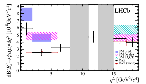
Differential branching fraction of the decay $ B ^0_ s \rightarrow \phi\mu ^+\mu ^- $,
overlaid with SM predictions [4,5] indicated by blue shaded boxes. The vetoes excluding the charmonium resonances are indicated by
grey areas.
|
diffBR[..].pdf [11 KiB]
HiDef png [105 KiB]
Thumbnail [103 KiB]
*.C file
|

|
|
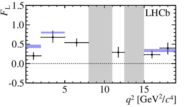
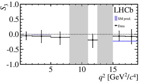
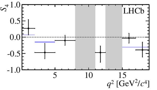
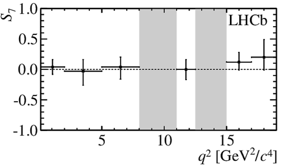
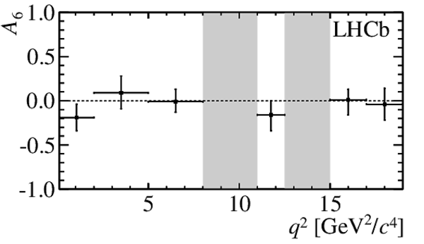
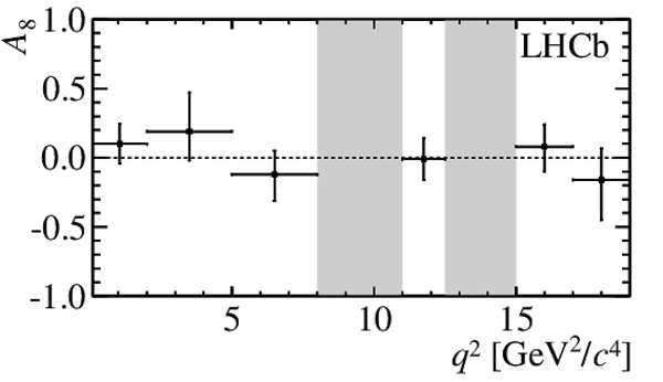
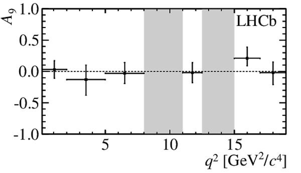
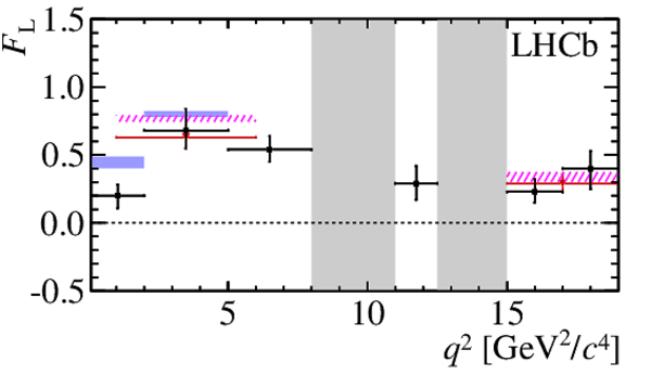
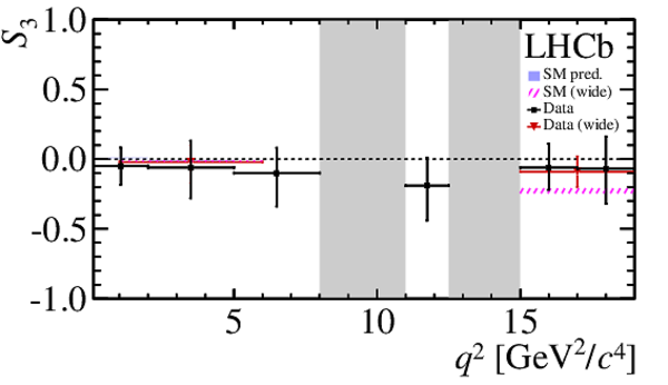
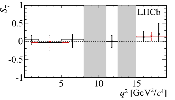
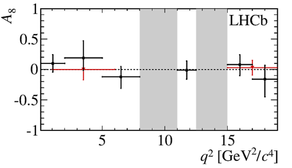
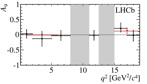
$ C P$ -averaged angular observables $F_{\rm L}$ and $S_{3,4,7}$ and $ C P$ asymmetries $A_{5,6,8,9}$ shown by black dots,
overlaid with SM predictions [4,5], where available, indicated as blue shaded boxes. The vetoes excluding the charmonium resonances are indicated by
grey areas.
|
FL_plot.pdf [7 KiB]
HiDef png [88 KiB]
Thumbnail [91 KiB]
*.C file
|
|
S3_plot.pdf [8 KiB]
HiDef png [99 KiB]
Thumbnail [99 KiB]
*.C file
|
|
S4_plot.pdf [7 KiB]
HiDef png [91 KiB]
Thumbnail [91 KiB]
*.C file
|
|
S7_plot.pdf [13 KiB]
HiDef png [65 KiB]
Thumbnail [39 KiB]
*.C file
|
|
A5_plot.pdf [13 KiB]
HiDef png [66 KiB]
Thumbnail [40 KiB]
*.C file
|

|
A6_plot.pdf [13 KiB]
HiDef png [65 KiB]
Thumbnail [39 KiB]
*.C file
|
|
A8_plot.pdf [13 KiB]
HiDef png [66 KiB]
Thumbnail [40 KiB]
*.C file
|
|
A9_plot.pdf [13 KiB]
HiDef png [66 KiB]
Thumbnail [40 KiB]
*.C file
|
|
|
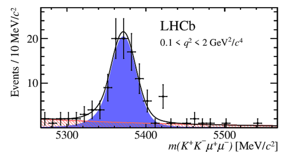
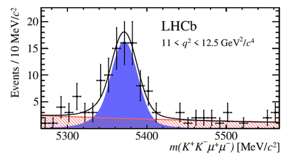
Invariant mass distributions for $ B ^0_ s \rightarrow \phi\mu ^+\mu ^- $ signal decays in bins of $q^2$. The signal component is shown by the solid blue area, the background component by the shaded red area.
|
m0.pdf [22 KiB]
HiDef png [189 KiB]
Thumbnail [141 KiB]
*.C file
|
|
m1.pdf [23 KiB]
HiDef png [241 KiB]
Thumbnail [184 KiB]
*.C file
|

|
m2.pdf [23 KiB]
HiDef png [216 KiB]
Thumbnail [167 KiB]
*.C file
|

|
m3.pdf [22 KiB]
HiDef png [226 KiB]
Thumbnail [174 KiB]
*.C file
|
|
m4.pdf [22 KiB]
HiDef png [198 KiB]
Thumbnail [150 KiB]
*.C file
|

|
m5.pdf [22 KiB]
HiDef png [168 KiB]
Thumbnail [133 KiB]
*.C file
|
|
m6.pdf [23 KiB]
HiDef png [253 KiB]
Thumbnail [189 KiB]
*.C file
|

|
m7.pdf [23 KiB]
HiDef png [186 KiB]
Thumbnail [152 KiB]
*.C file
|
|
|
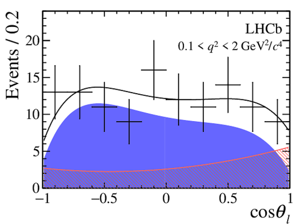
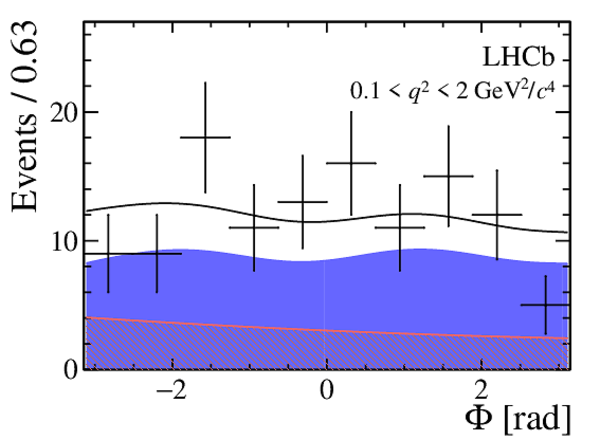
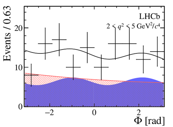
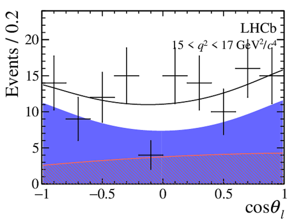
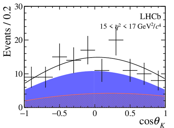
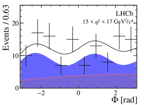
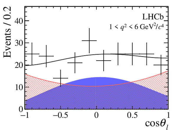
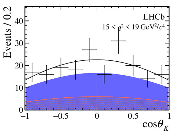
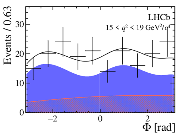
One-dimensional projections of the fit to the angles $\cos\theta_l$, $\cos\theta_K$, $\Phi$ in bins of $q^2$. The signal component is shown
by the solid blue area, the background component by the shaded red area.
|
costhe[..].pdf [16 KiB]
HiDef png [321 KiB]
Thumbnail [230 KiB]
*.C file
|
|
costhe[..].pdf [16 KiB]
HiDef png [288 KiB]
Thumbnail [205 KiB]
*.C file
|

|
phi0_pmm.pdf [16 KiB]
HiDef png [286 KiB]
Thumbnail [200 KiB]
*.C file
|
|
costhe[..].pdf [16 KiB]
HiDef png [418 KiB]
Thumbnail [283 KiB]
*.C file
|

|
costhe[..].pdf [16 KiB]
HiDef png [410 KiB]
Thumbnail [274 KiB]
*.C file
|

|
phi1_pmm.pdf [16 KiB]
HiDef png [463 KiB]
Thumbnail [303 KiB]
*.C file
|
|
costhe[..].pdf [16 KiB]
HiDef png [465 KiB]
Thumbnail [305 KiB]
*.C file
|

|
costhe[..].pdf [16 KiB]
HiDef png [412 KiB]
Thumbnail [280 KiB]
*.C file
|

|
phi2_pmm.pdf [16 KiB]
HiDef png [425 KiB]
Thumbnail [288 KiB]
*.C file
|

|
costhe[..].pdf [16 KiB]
HiDef png [377 KiB]
Thumbnail [256 KiB]
*.C file
|
|
costhe[..].pdf [16 KiB]
HiDef png [428 KiB]
Thumbnail [300 KiB]
*.C file
|
|
phi4_pmm.pdf [16 KiB]
HiDef png [374 KiB]
Thumbnail [251 KiB]
*.C file
|
|
|
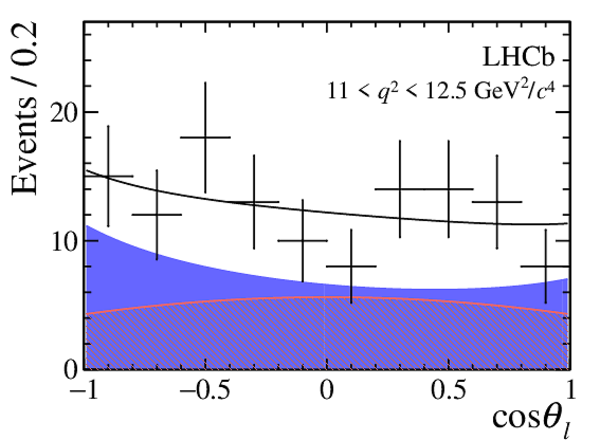
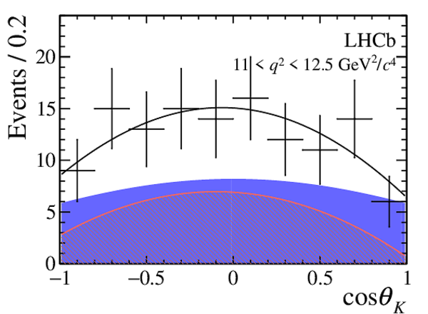
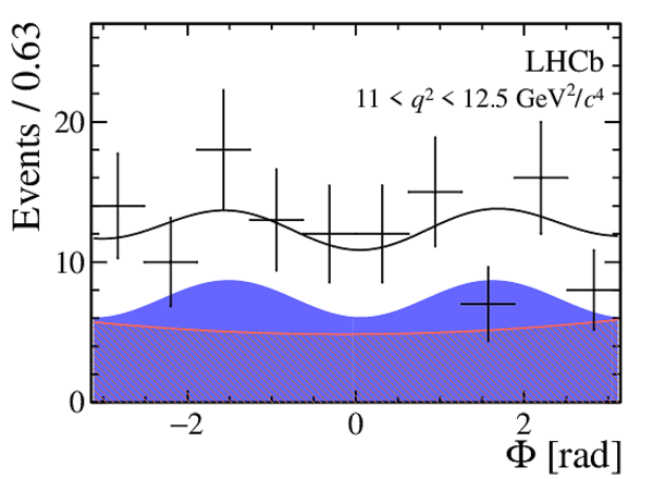
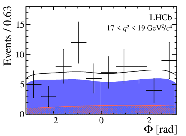
One-dimensional projections of the fit to the angles $\cos\theta_l$, $\cos\theta_K$, $\Phi$ in bins of $q^2$. The signal component is shown
by the solid blue area, the background component by the shaded red area.
|
costhe[..].pdf [16 KiB]
HiDef png [347 KiB]
Thumbnail [246 KiB]
*.C file
|
|
costhe[..].pdf [16 KiB]
HiDef png [304 KiB]
Thumbnail [221 KiB]
*.C file
|
|
phi6_pmm.pdf [16 KiB]
HiDef png [322 KiB]
Thumbnail [227 KiB]
*.C file
|
|
costhe[..].pdf [16 KiB]
HiDef png [251 KiB]
Thumbnail [185 KiB]
*.C file
|

|
costhe[..].pdf [16 KiB]
HiDef png [256 KiB]
Thumbnail [192 KiB]
*.C file
|

|
phi7_pmm.pdf [16 KiB]
HiDef png [234 KiB]
Thumbnail [174 KiB]
*.C file
|
|
costhe[..].pdf [16 KiB]
HiDef png [459 KiB]
Thumbnail [309 KiB]
*.C file
|
|
costhe[..].pdf [16 KiB]
HiDef png [447 KiB]
Thumbnail [301 KiB]
*.C file
|

|
phi9_pmm.pdf [16 KiB]
HiDef png [439 KiB]
Thumbnail [293 KiB]
*.C file
|

|
costhe[..].pdf [16 KiB]
HiDef png [338 KiB]
Thumbnail [239 KiB]
*.C file
|

|
costhe[..].pdf [16 KiB]
HiDef png [297 KiB]
Thumbnail [220 KiB]
*.C file
|
|
phi11_pmm.pdf [16 KiB]
HiDef png [325 KiB]
Thumbnail [232 KiB]
*.C file
|
|
|
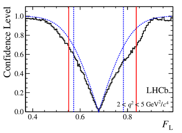
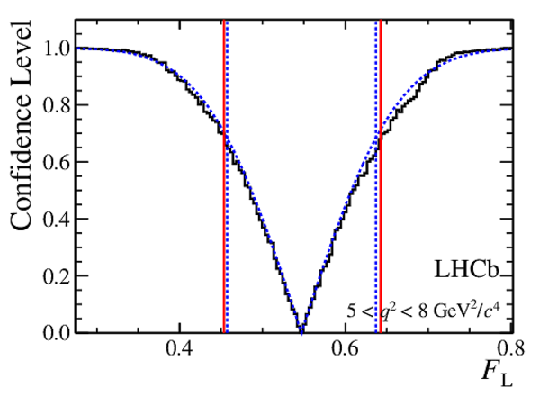
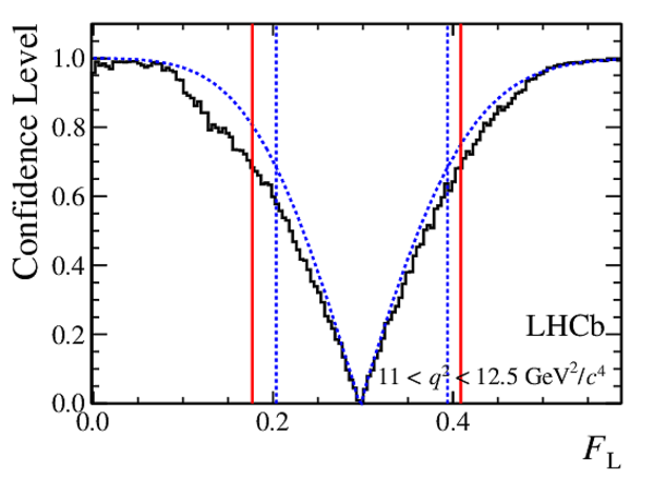
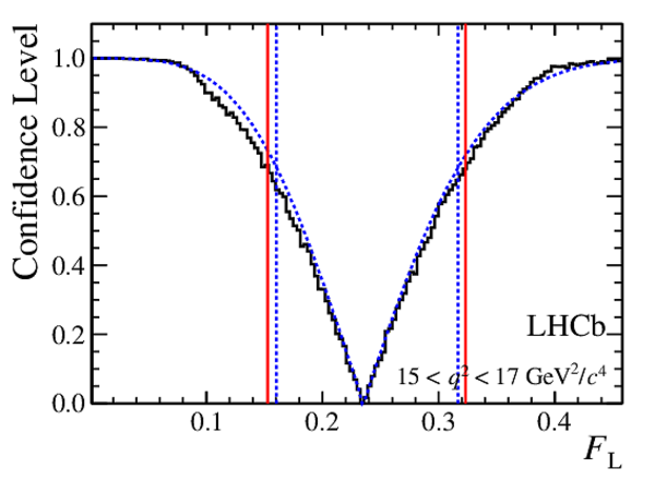
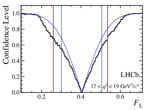
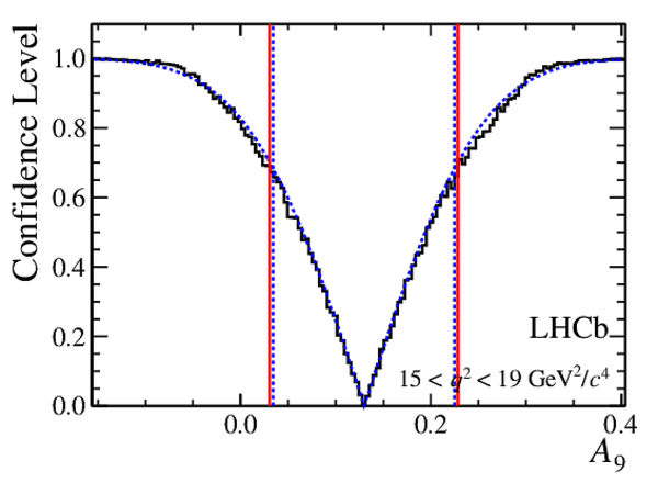
Confidence level obtained from a likelihood scan (shaded blue) and from the Feldman-Cousins method (solid black).
The shaded blue and solid red vertical lines indicate the corresponding $68\%$ CL intervals obtained from the likelihood scan and the Feldman-Cousins method, respectively.
|
clJ1c0.pdf [9 KiB]
HiDef png [179 KiB]
Thumbnail [158 KiB]
*.C file
|

|
clJ1c1.pdf [9 KiB]
HiDef png [174 KiB]
Thumbnail [157 KiB]
*.C file
|
|
clJ1c2.pdf [9 KiB]
HiDef png [172 KiB]
Thumbnail [149 KiB]
*.C file
|
|
clJ1c4.pdf [9 KiB]
HiDef png [171 KiB]
Thumbnail [156 KiB]
*.C file
|
|
clJ1c6.pdf [9 KiB]
HiDef png [173 KiB]
Thumbnail [157 KiB]
*.C file
|
|
clJ1c7.pdf [9 KiB]
HiDef png [172 KiB]
Thumbnail [153 KiB]
*.C file
|
|
clJ1c9.pdf [9 KiB]
HiDef png [177 KiB]
Thumbnail [157 KiB]
*.C file
|

|
clJ1c11.pdf [9 KiB]
HiDef png [177 KiB]
Thumbnail [150 KiB]
*.C file
|

|
|
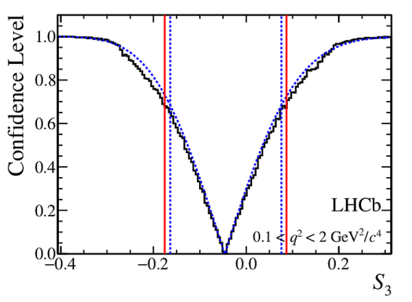
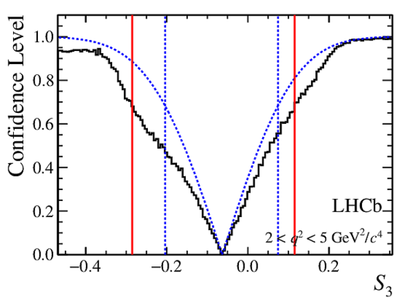
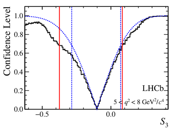
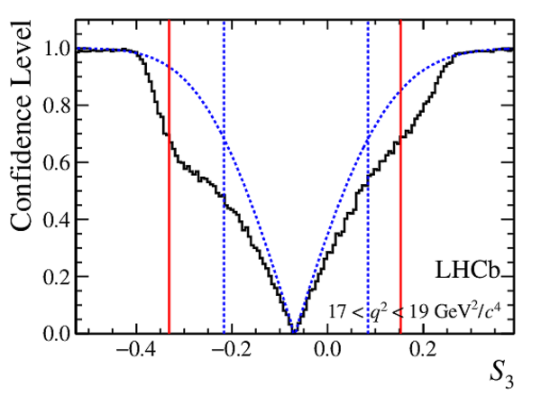
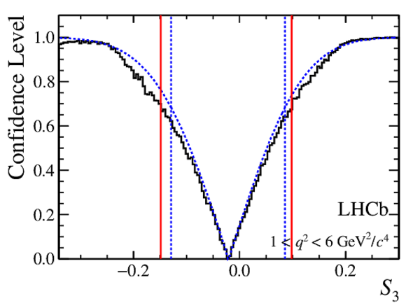
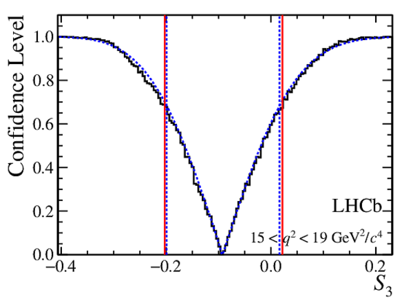
Confidence level obtained from a likelihood scan (shaded blue) and from a Feldman-Cousins method (solid black).
The shaded blue and solid red vertical lines indicate the corresponding $68\%$ CL intervals obtained from the likelihood scan and the Feldman-Cousins method, respectively.
|
clJ30.pdf [10 KiB]
HiDef png [176 KiB]
Thumbnail [151 KiB]
*.C file
|
|
clJ31.pdf [10 KiB]
HiDef png [175 KiB]
Thumbnail [164 KiB]
*.C file
|
|
clJ32.pdf [10 KiB]
HiDef png [169 KiB]
Thumbnail [148 KiB]
*.C file
|
|
clJ34.pdf [10 KiB]
HiDef png [179 KiB]
Thumbnail [166 KiB]
*.C file
|

|
clJ36.pdf [10 KiB]
HiDef png [176 KiB]
Thumbnail [156 KiB]
*.C file
|

|
clJ37.pdf [10 KiB]
HiDef png [176 KiB]
Thumbnail [161 KiB]
*.C file
|
|
clJ39.pdf [10 KiB]
HiDef png [171 KiB]
Thumbnail [150 KiB]
*.C file
|
|
clJ311.pdf [10 KiB]
HiDef png [175 KiB]
Thumbnail [147 KiB]
*.C file
|
|
|
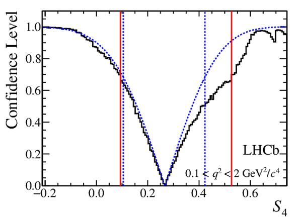
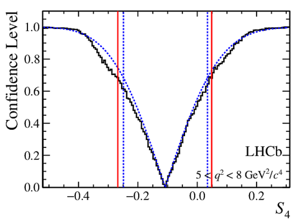
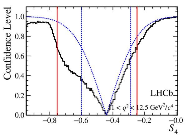
Confidence level obtained from a likelihood scan (shaded blue) and from a Feldman-Cousins method (solid black).
The shaded blue and solid red vertical lines indicate the corresponding $68\%$ CL intervals obtained from the likelihood scan and the Feldman-Cousins method, respectively.
|
clJ40.pdf [10 KiB]
HiDef png [179 KiB]
Thumbnail [160 KiB]
*.C file
|
|
clJ41.pdf [10 KiB]
HiDef png [174 KiB]
Thumbnail [158 KiB]
*.C file
|

|
clJ42.pdf [10 KiB]
HiDef png [174 KiB]
Thumbnail [154 KiB]
*.C file
|
|
clJ44.pdf [10 KiB]
HiDef png [177 KiB]
Thumbnail [169 KiB]
*.C file
|
|
clJ46.pdf [10 KiB]
HiDef png [173 KiB]
Thumbnail [152 KiB]
*.C file
|

|
clJ47.pdf [10 KiB]
HiDef png [169 KiB]
Thumbnail [151 KiB]
*.C file
|

|
clJ49.pdf [9 KiB]
HiDef png [169 KiB]
Thumbnail [153 KiB]
*.C file
|

|
clJ411.pdf [10 KiB]
HiDef png [172 KiB]
Thumbnail [151 KiB]
*.C file
|

|
|
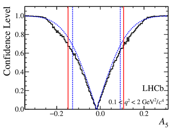
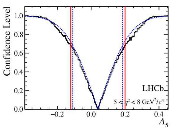
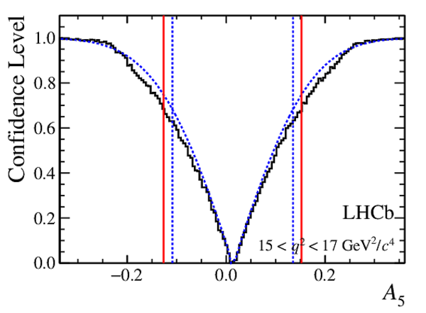
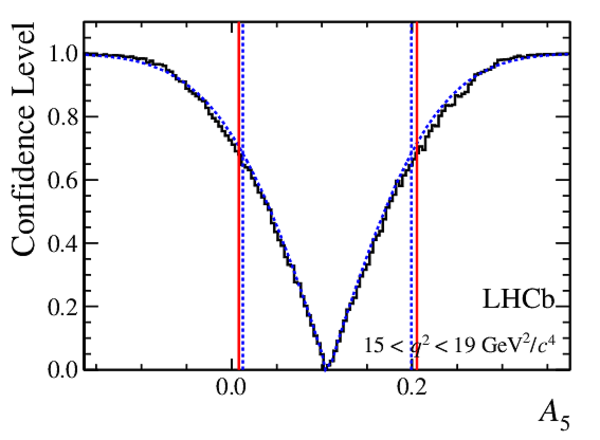
Confidence level obtained from a likelihood scan (shaded blue) and from a Feldman-Cousins method (solid black).
The shaded blue and solid red vertical lines indicate the corresponding $68\%$ CL intervals obtained from the likelihood scan and the Feldman-Cousins method, respectively.
|
clJ50.pdf [10 KiB]
HiDef png [169 KiB]
Thumbnail [153 KiB]
*.C file
|
|
clJ51.pdf [9 KiB]
HiDef png [170 KiB]
Thumbnail [156 KiB]
*.C file
|

|
clJ52.pdf [10 KiB]
HiDef png [171 KiB]
Thumbnail [156 KiB]
*.C file
|
|
clJ54.pdf [10 KiB]
HiDef png [178 KiB]
Thumbnail [165 KiB]
*.C file
|

|
clJ56.pdf [10 KiB]
HiDef png [172 KiB]
Thumbnail [153 KiB]
*.C file
|
|
clJ57.pdf [10 KiB]
HiDef png [173 KiB]
Thumbnail [163 KiB]
*.C file
|

|
clJ59.pdf [9 KiB]
HiDef png [171 KiB]
Thumbnail [153 KiB]
*.C file
|

|
clJ511.pdf [9 KiB]
HiDef png [171 KiB]
Thumbnail [144 KiB]
*.C file
|
|
|
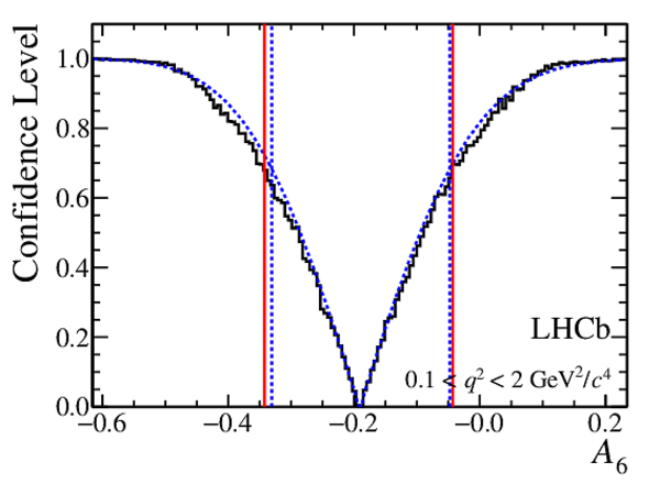
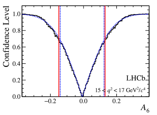
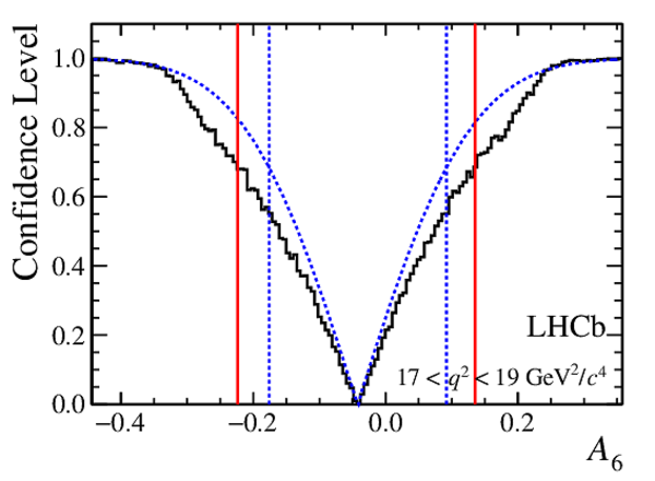
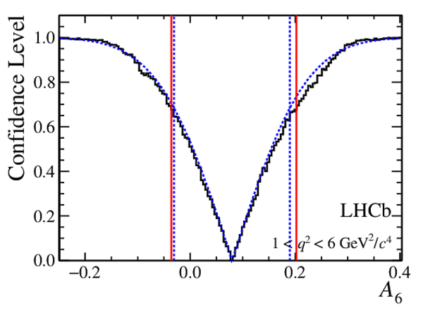
Confidence level obtained from a likelihood scan (shaded blue) and from a Feldman-Cousins method (solid black).
The shaded blue and solid red vertical lines indicate the corresponding $68\%$ CL intervals obtained from the likelihood scan and the Feldman-Cousins method, respectively.
|
clJ6s0.pdf [10 KiB]
HiDef png [177 KiB]
Thumbnail [154 KiB]
*.C file
|
|
clJ6s1.pdf [10 KiB]
HiDef png [176 KiB]
Thumbnail [160 KiB]
*.C file
|

|
clJ6s2.pdf [10 KiB]
HiDef png [171 KiB]
Thumbnail [148 KiB]
*.C file
|

|
clJ6s4.pdf [10 KiB]
HiDef png [177 KiB]
Thumbnail [162 KiB]
*.C file
|

|
clJ6s6.pdf [10 KiB]
HiDef png [169 KiB]
Thumbnail [147 KiB]
*.C file
|
|
clJ6s7.pdf [10 KiB]
HiDef png [173 KiB]
Thumbnail [160 KiB]
*.C file
|
|
clJ6s9.pdf [9 KiB]
HiDef png [173 KiB]
Thumbnail [150 KiB]
*.C file
|
|
clJ6s11.pdf [10 KiB]
HiDef png [181 KiB]
Thumbnail [150 KiB]
*.C file
|

|
|
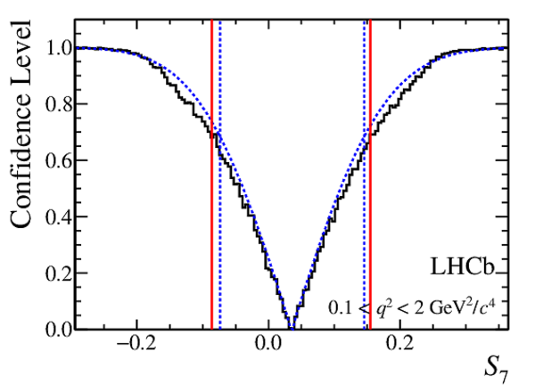
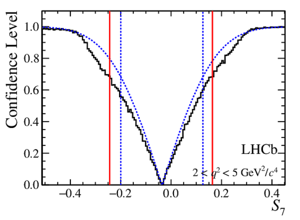
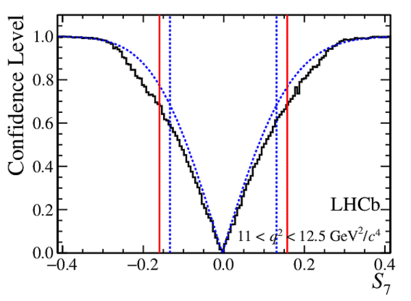
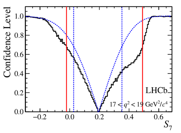
Confidence level obtained from a likelihood scan (shaded blue) and from a Feldman-Cousins method (solid black).
The shaded blue and solid red vertical lines indicate the corresponding $68\%$ CL intervals obtained from the likelihood scan and the Feldman-Cousins method, respectively.
|
clJ70.pdf [9 KiB]
HiDef png [172 KiB]
Thumbnail [151 KiB]
*.C file
|
|
clJ71.pdf [10 KiB]
HiDef png [179 KiB]
Thumbnail [161 KiB]
*.C file
|
|
clJ72.pdf [10 KiB]
HiDef png [178 KiB]
Thumbnail [160 KiB]
*.C file
|

|
clJ74.pdf [10 KiB]
HiDef png [177 KiB]
Thumbnail [160 KiB]
*.C file
|
|
clJ76.pdf [10 KiB]
HiDef png [176 KiB]
Thumbnail [155 KiB]
*.C file
|

|
clJ77.pdf [10 KiB]
HiDef png [180 KiB]
Thumbnail [167 KiB]
*.C file
|
|
clJ79.pdf [10 KiB]
HiDef png [174 KiB]
Thumbnail [150 KiB]
*.C file
|

|
clJ711.pdf [9 KiB]
HiDef png [176 KiB]
Thumbnail [150 KiB]
*.C file
|

|
|
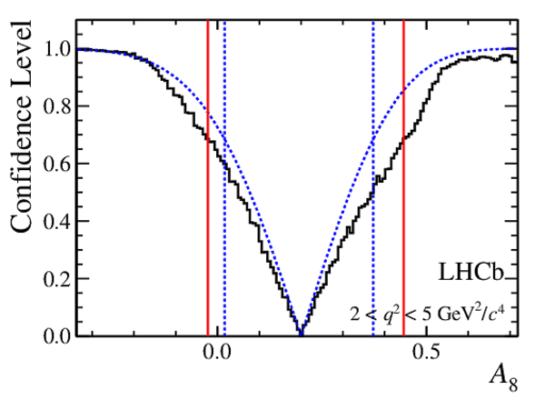
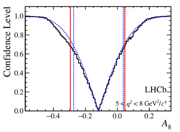
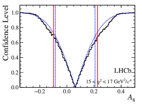
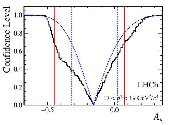
Confidence level obtained from a likelihood scan (shaded blue) and from a Feldman-Cousins method (solid black).
The shaded blue and solid red vertical lines indicate the corresponding $68\%$ CL intervals obtained from the likelihood scan and the Feldman-Cousins method, respectively.
|
clJ80.pdf [10 KiB]
HiDef png [176 KiB]
Thumbnail [155 KiB]
*.C file
|

|
clJ81.pdf [9 KiB]
HiDef png [170 KiB]
Thumbnail [151 KiB]
*.C file
|
|
clJ82.pdf [10 KiB]
HiDef png [174 KiB]
Thumbnail [155 KiB]
*.C file
|
|
clJ84.pdf [10 KiB]
HiDef png [170 KiB]
Thumbnail [153 KiB]
*.C file
|

|
clJ86.pdf [10 KiB]
HiDef png [172 KiB]
Thumbnail [158 KiB]
*.C file
|
|
clJ87.pdf [10 KiB]
HiDef png [163 KiB]
Thumbnail [154 KiB]
*.C file
|
|
clJ89.pdf [10 KiB]
HiDef png [179 KiB]
Thumbnail [157 KiB]
*.C file
|

|
clJ811.pdf [10 KiB]
HiDef png [176 KiB]
Thumbnail [154 KiB]
*.C file
|

|
|
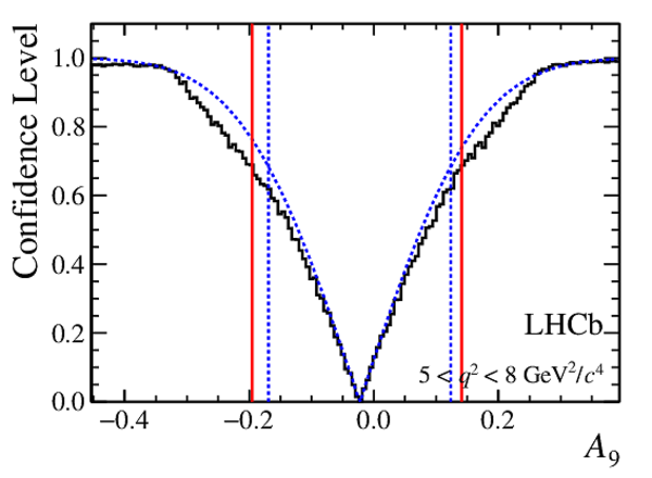
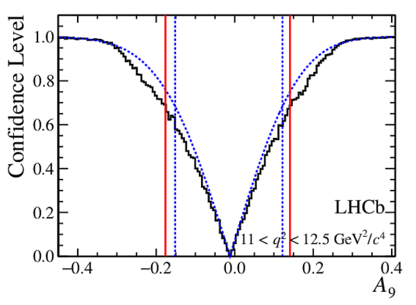
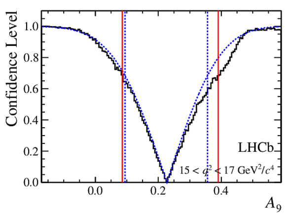
Confidence level obtained from a likelihood scan (shaded blue) and from a Feldman-Cousins method (solid black).
The shaded blue and solid red vertical lines indicate the corresponding $68\%$ CL intervals obtained from the likelihood scan and the Feldman-Cousins method, respectively.
|
clJ90.pdf [10 KiB]
HiDef png [175 KiB]
Thumbnail [152 KiB]
*.C file
|

|
clJ91.pdf [10 KiB]
HiDef png [170 KiB]
Thumbnail [152 KiB]
*.C file
|

|
clJ92.pdf [10 KiB]
HiDef png [175 KiB]
Thumbnail [159 KiB]
*.C file
|
|
clJ94.pdf [10 KiB]
HiDef png [179 KiB]
Thumbnail [162 KiB]
*.C file
|
|
clJ96.pdf [9 KiB]
HiDef png [172 KiB]
Thumbnail [152 KiB]
*.C file
|
|
clJ97.pdf [10 KiB]
HiDef png [175 KiB]
Thumbnail [158 KiB]
*.C file
|

|
clJ99.pdf [10 KiB]
HiDef png [173 KiB]
Thumbnail [150 KiB]
*.C file
|

|
clJ911.pdf [9 KiB]
HiDef png [173 KiB]
Thumbnail [150 KiB]
*.C file
|
|
|
Animated gif made out of all figures.
|
PAPER-2015-023.gif
Thumbnail
|

|
|
The signal yields for $ B ^0_ s \rightarrow \phi\mu ^+\mu ^- $ decays, as well as the differential branching fraction relative to the normalisation mode
and the absolute differential branching fraction, in bins of $q^2$. The given uncertainties are (from left to right) statistical, systematic, and the uncertainty on the branching fraction of the normalisation mode.
|
Table_1.pdf [74 KiB]
HiDef png [88 KiB]
Thumbnail [41 KiB]
tex code
|

|
|
Systematic uncertainties $[10^{-5}\mathrm{ Ge V} ^{-2}c^{4}]$ on the branching fraction ratio ${\rm d}\cal B ( B ^0_ s \rightarrow \phi\mu ^+\mu ^- )/\cal B ( B ^0_ s \rightarrow { J \mskip -3mu/\mskip -2mu\psi \mskip 2mu} \phi){\rm
d} q^2 $ per bin of $ q^2$ $[ {\mathrm{ Ge V^2 /}c^4} ]$.
|
Table_2.pdf [46 KiB]
HiDef png [86 KiB]
Thumbnail [37 KiB]
tex code
|

|
|
(Top) $ C P$ -averaged angular observables $F_{\rm L}$ and $S_{3,4,7}$ and (bottom) $ C P$ asymmetries $A_{5,6,8,9}$ obtained from the unbinned maximum likelihood fit, where
the first uncertainty is statistical and the second is systematic.
|
Table_3.pdf [51 KiB]
HiDef png [74 KiB]
Thumbnail [27 KiB]
tex code
|

|
|
Correlation matrices for the $q^2$ bins $0.1<q^2<2.0 {\mathrm{ Ge V^2 /}c^4} $, $2.0<q^2<5.0 {\mathrm{ Ge V^2 /}c^4} $ and $5.0<q^2<8.0 {\mathrm{ Ge V^2 /}c^4} $.
|
Table_4.pdf [45 KiB]
HiDef png [44 KiB]
Thumbnail [15 KiB]
tex code
|

|
|
Correlation matrices for the $q^2$ bins $11.0<q^2<12.5 {\mathrm{ Ge V^2 /}c^4} $, $15.0<q^2<17.0 {\mathrm{ Ge V^2 /}c^4} $ and $17.0<q^2<19.0 {\mathrm{ Ge V^2 /}c^4} $.
|
Table_5.pdf [45 KiB]
HiDef png [45 KiB]
Thumbnail [13 KiB]
tex code
|

|
|
Correlation matrices for the $q^2$ bins $1.0<q^2<6.0 {\mathrm{ Ge V^2 /}c^4} $ and $15.0<q^2<19.0 {\mathrm{ Ge V^2 /}c^4} $.
|
Table_6.pdf [45 KiB]
HiDef png [53 KiB]
Thumbnail [20 KiB]
tex code
|

|
![HiDef png [15 KiB]](Directory_LHCb-PAPER-2015-023/hidef_Fig_1.png)
![HiDef png [399 KiB]](Directory_LHCb-PAPER-2015-023/hidef_mbvsq2.png)
![HiDef png [218 KiB]](Directory_LHCb-PAPER-2015-023/hidef_m_fullq2.png)
![HiDef png [149 KiB]](Directory_LHCb-PAPER-2015-023/hidef_m_res.png)
![HiDef png [105 KiB]](Directory_LHCb-PAPER-2015-023/hidef_diffBR_plot.png)
![HiDef png [88 KiB]](Directory_LHCb-PAPER-2015-023/hidef_FL_plot.png)
![HiDef png [99 KiB]](Directory_LHCb-PAPER-2015-023/hidef_S3_plot.png)
![HiDef png [91 KiB]](Directory_LHCb-PAPER-2015-023/hidef_S4_plot.png)
![HiDef png [65 KiB]](Directory_LHCb-PAPER-2015-023/hidef_S7_plot.png)
![HiDef png [66 KiB]](Directory_LHCb-PAPER-2015-023/hidef_A5_plot.png)
![HiDef png [65 KiB]](Directory_LHCb-PAPER-2015-023/hidef_A6_plot.png)
![HiDef png [66 KiB]](Directory_LHCb-PAPER-2015-023/hidef_A8_plot.png)
![HiDef png [66 KiB]](Directory_LHCb-PAPER-2015-023/hidef_A9_plot.png)
![HiDef png [189 KiB]](Directory_LHCb-PAPER-2015-023/hidef_m0.png)
![HiDef png [241 KiB]](Directory_LHCb-PAPER-2015-023/hidef_m1.png)
![HiDef png [216 KiB]](Directory_LHCb-PAPER-2015-023/hidef_m2.png)
![HiDef png [226 KiB]](Directory_LHCb-PAPER-2015-023/hidef_m3.png)
![HiDef png [198 KiB]](Directory_LHCb-PAPER-2015-023/hidef_m4.png)
![HiDef png [168 KiB]](Directory_LHCb-PAPER-2015-023/hidef_m5.png)
![HiDef png [253 KiB]](Directory_LHCb-PAPER-2015-023/hidef_m6.png)
![HiDef png [186 KiB]](Directory_LHCb-PAPER-2015-023/hidef_m7.png)
![HiDef png [321 KiB]](Directory_LHCb-PAPER-2015-023/hidef_costhetal0_pmm.png)
![HiDef png [288 KiB]](Directory_LHCb-PAPER-2015-023/hidef_costhetak0_pmm.png)
![HiDef png [286 KiB]](Directory_LHCb-PAPER-2015-023/hidef_phi0_pmm.png)
![HiDef png [418 KiB]](Directory_LHCb-PAPER-2015-023/hidef_costhetal1_pmm.png)
![HiDef png [410 KiB]](Directory_LHCb-PAPER-2015-023/hidef_costhetak1_pmm.png)
![HiDef png [463 KiB]](Directory_LHCb-PAPER-2015-023/hidef_phi1_pmm.png)
![HiDef png [465 KiB]](Directory_LHCb-PAPER-2015-023/hidef_costhetal2_pmm.png)
![HiDef png [412 KiB]](Directory_LHCb-PAPER-2015-023/hidef_costhetak2_pmm.png)
![HiDef png [425 KiB]](Directory_LHCb-PAPER-2015-023/hidef_phi2_pmm.png)
![HiDef png [377 KiB]](Directory_LHCb-PAPER-2015-023/hidef_costhetal4_pmm.png)
![HiDef png [428 KiB]](Directory_LHCb-PAPER-2015-023/hidef_costhetak4_pmm.png)
![HiDef png [374 KiB]](Directory_LHCb-PAPER-2015-023/hidef_phi4_pmm.png)
![HiDef png [347 KiB]](Directory_LHCb-PAPER-2015-023/hidef_costhetal6_pmm.png)
![HiDef png [304 KiB]](Directory_LHCb-PAPER-2015-023/hidef_costhetak6_pmm.png)
![HiDef png [322 KiB]](Directory_LHCb-PAPER-2015-023/hidef_phi6_pmm.png)
![HiDef png [251 KiB]](Directory_LHCb-PAPER-2015-023/hidef_costhetal7_pmm.png)
![HiDef png [256 KiB]](Directory_LHCb-PAPER-2015-023/hidef_costhetak7_pmm.png)
![HiDef png [234 KiB]](Directory_LHCb-PAPER-2015-023/hidef_phi7_pmm.png)
![HiDef png [459 KiB]](Directory_LHCb-PAPER-2015-023/hidef_costhetal9_pmm.png)
![HiDef png [447 KiB]](Directory_LHCb-PAPER-2015-023/hidef_costhetak9_pmm.png)
![HiDef png [439 KiB]](Directory_LHCb-PAPER-2015-023/hidef_phi9_pmm.png)
![HiDef png [338 KiB]](Directory_LHCb-PAPER-2015-023/hidef_costhetal11_pmm.png)
![HiDef png [297 KiB]](Directory_LHCb-PAPER-2015-023/hidef_costhetak11_pmm.png)
![HiDef png [325 KiB]](Directory_LHCb-PAPER-2015-023/hidef_phi11_pmm.png)
![HiDef png [179 KiB]](Directory_LHCb-PAPER-2015-023/hidef_clJ1c0.png)
![HiDef png [174 KiB]](Directory_LHCb-PAPER-2015-023/hidef_clJ1c1.png)
![HiDef png [172 KiB]](Directory_LHCb-PAPER-2015-023/hidef_clJ1c2.png)
![HiDef png [171 KiB]](Directory_LHCb-PAPER-2015-023/hidef_clJ1c4.png)
![HiDef png [173 KiB]](Directory_LHCb-PAPER-2015-023/hidef_clJ1c6.png)
![HiDef png [172 KiB]](Directory_LHCb-PAPER-2015-023/hidef_clJ1c7.png)
![HiDef png [177 KiB]](Directory_LHCb-PAPER-2015-023/hidef_clJ1c9.png)
![HiDef png [177 KiB]](Directory_LHCb-PAPER-2015-023/hidef_clJ1c11.png)
![HiDef png [176 KiB]](Directory_LHCb-PAPER-2015-023/hidef_clJ30.png)
![HiDef png [175 KiB]](Directory_LHCb-PAPER-2015-023/hidef_clJ31.png)
![HiDef png [169 KiB]](Directory_LHCb-PAPER-2015-023/hidef_clJ32.png)
![HiDef png [179 KiB]](Directory_LHCb-PAPER-2015-023/hidef_clJ34.png)
![HiDef png [176 KiB]](Directory_LHCb-PAPER-2015-023/hidef_clJ36.png)
![HiDef png [176 KiB]](Directory_LHCb-PAPER-2015-023/hidef_clJ37.png)
![HiDef png [171 KiB]](Directory_LHCb-PAPER-2015-023/hidef_clJ39.png)
![HiDef png [175 KiB]](Directory_LHCb-PAPER-2015-023/hidef_clJ311.png)
![HiDef png [179 KiB]](Directory_LHCb-PAPER-2015-023/hidef_clJ40.png)
![HiDef png [174 KiB]](Directory_LHCb-PAPER-2015-023/hidef_clJ41.png)
![HiDef png [174 KiB]](Directory_LHCb-PAPER-2015-023/hidef_clJ42.png)
![HiDef png [177 KiB]](Directory_LHCb-PAPER-2015-023/hidef_clJ44.png)
![HiDef png [173 KiB]](Directory_LHCb-PAPER-2015-023/hidef_clJ46.png)
![HiDef png [169 KiB]](Directory_LHCb-PAPER-2015-023/hidef_clJ47.png)
![HiDef png [169 KiB]](Directory_LHCb-PAPER-2015-023/hidef_clJ49.png)
![HiDef png [172 KiB]](Directory_LHCb-PAPER-2015-023/hidef_clJ411.png)
![HiDef png [169 KiB]](Directory_LHCb-PAPER-2015-023/hidef_clJ50.png)
![HiDef png [170 KiB]](Directory_LHCb-PAPER-2015-023/hidef_clJ51.png)
![HiDef png [171 KiB]](Directory_LHCb-PAPER-2015-023/hidef_clJ52.png)
![HiDef png [178 KiB]](Directory_LHCb-PAPER-2015-023/hidef_clJ54.png)
![HiDef png [172 KiB]](Directory_LHCb-PAPER-2015-023/hidef_clJ56.png)
![HiDef png [173 KiB]](Directory_LHCb-PAPER-2015-023/hidef_clJ57.png)
![HiDef png [171 KiB]](Directory_LHCb-PAPER-2015-023/hidef_clJ59.png)
![HiDef png [171 KiB]](Directory_LHCb-PAPER-2015-023/hidef_clJ511.png)
![HiDef png [177 KiB]](Directory_LHCb-PAPER-2015-023/hidef_clJ6s0.png)
![HiDef png [176 KiB]](Directory_LHCb-PAPER-2015-023/hidef_clJ6s1.png)
![HiDef png [171 KiB]](Directory_LHCb-PAPER-2015-023/hidef_clJ6s2.png)
![HiDef png [177 KiB]](Directory_LHCb-PAPER-2015-023/hidef_clJ6s4.png)
![HiDef png [169 KiB]](Directory_LHCb-PAPER-2015-023/hidef_clJ6s6.png)
![HiDef png [173 KiB]](Directory_LHCb-PAPER-2015-023/hidef_clJ6s7.png)
![HiDef png [173 KiB]](Directory_LHCb-PAPER-2015-023/hidef_clJ6s9.png)
![HiDef png [181 KiB]](Directory_LHCb-PAPER-2015-023/hidef_clJ6s11.png)
![HiDef png [172 KiB]](Directory_LHCb-PAPER-2015-023/hidef_clJ70.png)
![HiDef png [179 KiB]](Directory_LHCb-PAPER-2015-023/hidef_clJ71.png)
![HiDef png [178 KiB]](Directory_LHCb-PAPER-2015-023/hidef_clJ72.png)
![HiDef png [177 KiB]](Directory_LHCb-PAPER-2015-023/hidef_clJ74.png)
![HiDef png [176 KiB]](Directory_LHCb-PAPER-2015-023/hidef_clJ76.png)
![HiDef png [180 KiB]](Directory_LHCb-PAPER-2015-023/hidef_clJ77.png)
![HiDef png [174 KiB]](Directory_LHCb-PAPER-2015-023/hidef_clJ79.png)
![HiDef png [176 KiB]](Directory_LHCb-PAPER-2015-023/hidef_clJ711.png)
![HiDef png [176 KiB]](Directory_LHCb-PAPER-2015-023/hidef_clJ80.png)
![HiDef png [170 KiB]](Directory_LHCb-PAPER-2015-023/hidef_clJ81.png)
![HiDef png [174 KiB]](Directory_LHCb-PAPER-2015-023/hidef_clJ82.png)
![HiDef png [170 KiB]](Directory_LHCb-PAPER-2015-023/hidef_clJ84.png)
![HiDef png [172 KiB]](Directory_LHCb-PAPER-2015-023/hidef_clJ86.png)
![HiDef png [163 KiB]](Directory_LHCb-PAPER-2015-023/hidef_clJ87.png)
![HiDef png [179 KiB]](Directory_LHCb-PAPER-2015-023/hidef_clJ89.png)
![HiDef png [176 KiB]](Directory_LHCb-PAPER-2015-023/hidef_clJ811.png)
![HiDef png [175 KiB]](Directory_LHCb-PAPER-2015-023/hidef_clJ90.png)
![HiDef png [170 KiB]](Directory_LHCb-PAPER-2015-023/hidef_clJ91.png)
![HiDef png [175 KiB]](Directory_LHCb-PAPER-2015-023/hidef_clJ92.png)
![HiDef png [179 KiB]](Directory_LHCb-PAPER-2015-023/hidef_clJ94.png)
![HiDef png [172 KiB]](Directory_LHCb-PAPER-2015-023/hidef_clJ96.png)
![HiDef png [175 KiB]](Directory_LHCb-PAPER-2015-023/hidef_clJ97.png)
![HiDef png [173 KiB]](Directory_LHCb-PAPER-2015-023/hidef_clJ99.png)
![HiDef png [173 KiB]](Directory_LHCb-PAPER-2015-023/hidef_clJ911.png)
![HiDef png [88 KiB]](Directory_LHCb-PAPER-2015-023/hidef_Table_1.png)
![HiDef png [86 KiB]](Directory_LHCb-PAPER-2015-023/hidef_Table_2.png)
![HiDef png [74 KiB]](Directory_LHCb-PAPER-2015-023/hidef_Table_3.png)
![HiDef png [44 KiB]](Directory_LHCb-PAPER-2015-023/hidef_Table_4.png)
![HiDef png [45 KiB]](Directory_LHCb-PAPER-2015-023/hidef_Table_5.png)
![HiDef png [53 KiB]](Directory_LHCb-PAPER-2015-023/hidef_Table_6.png)


![HiDef png [319 KiB]](Directory_LHCb-PAPER-2015-023/supplementary/hidef_Sup_fig1.png)
![HiDef png [239 KiB]](Directory_LHCb-PAPER-2015-023/supplementary/hidef_Sup_fig2.png)
![HiDef png [109 KiB]](Directory_LHCb-PAPER-2015-023/supplementary/hidef_Sup_fig3a.png)
![HiDef png [123 KiB]](Directory_LHCb-PAPER-2015-023/supplementary/hidef_Sup_fig3b.png)
![HiDef png [105 KiB]](Directory_LHCb-PAPER-2015-023/supplementary/hidef_Sup_fig3c.png)
![HiDef png [86 KiB]](Directory_LHCb-PAPER-2015-023/supplementary/hidef_Sup_fig3d.png)
![HiDef png [87 KiB]](Directory_LHCb-PAPER-2015-023/supplementary/hidef_Sup_fig3e.png)
![HiDef png [87 KiB]](Directory_LHCb-PAPER-2015-023/supplementary/hidef_Sup_fig3f.png)
![HiDef png [88 KiB]](Directory_LHCb-PAPER-2015-023/supplementary/hidef_Sup_fig3g.png)
![HiDef png [89 KiB]](Directory_LHCb-PAPER-2015-023/supplementary/hidef_Sup_fig3h.png)