Feynman diagrams for (a) $\Lambda ^0_ b \rightarrow { J \mskip -3mu/\mskip -2mu\psi \mskip 2mu} \Lambda ^*$ and (b) $\Lambda ^0_ b \rightarrow P_c^+ K^-$ decay.

Invariant mass of (a) $K^-p$ and (b) $ { J \mskip -3mu/\mskip -2mu\psi \mskip 2mu} p$ combinations from $\Lambda ^0_ b \rightarrow { J \mskip -3mu/\mskip -2mu\psi \mskip 2mu} K^-p$ decays. The solid (red) curve is the expectation from phase space. The background has been subtracted.

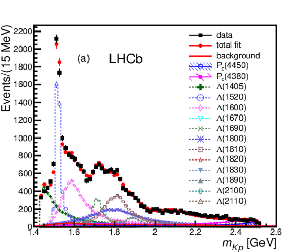
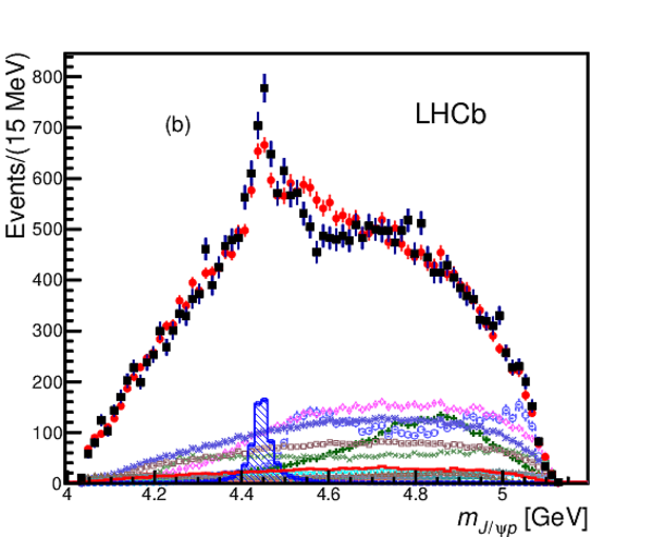
Fit projections for (a) $m_{Kp}$ and (b) $m_{ { J \mskip -3mu/\mskip -2mu\psi \mskip 2mu} p}$ for the reduced $\Lambda ^*$ model with two $P_c^+$ states (see Table 1). The data are shown as solid (black) squares, while the solid (red) points show the results of the fit. The solid (red) histogram shows the background distribution. The (blue) open squares with the shaded histogram represent the $P_c(4450)^+$ state, and the shaded histogram topped with (purple) filled squares represents the $P_c(4380)^+$ state. Each $\Lambda ^*$ component is also shown. The error bars on the points showing the fit results are due to simulation statistics.

Invariant mass spectrum of $ { J \mskip -3mu/\mskip -2mu\psi \mskip 2mu} K^-p$ combinations, with the total fit, signal and background components shown as solid (blue), solid (red) and dashed lines, respectively.

Invariant mass squared of $K^-p$ versus $ { J \mskip -3mu/\mskip -2mu\psi \mskip 2mu} p$ for candidates within $\pm15$ MeV of the $\Lambda ^0_ b $ mass.

Results for (a) $m_{Kp}$ and (b) $m_{ { J \mskip -3mu/\mskip -2mu\psi \mskip 2mu} p}$ for the extended $\Lambda ^*$ model fit without $P_c^+$ states. The data are shown as (black) squares with error bars, while the (red) circles show the results of the fit. The error bars on the points showing the fit results are due to simulation statistics.

Various decay angular distributions for the fit with two $P_c^+$ states. The data are shown as (black) squares, while the (red) circles show the results of the fit. Each fit component is also shown. The angles are defined in the text.

$m_{ { J \mskip -3mu/\mskip -2mu\psi \mskip 2mu} p}$ in various intervals of $m_{Kp}$ for the fit with two $P_c^+$ states: (a) $m_{Kp}<1.55$ GeV, (b) $1.55<m_{Kp}<1.70$ GeV, (c) $1.70<m_{Kp}<2.00$ GeV, and (d) $m_{Kp}>2.00$ GeV. The data are shown as (black) squares with error bars, while the (red) circles show the results of the fit. The blue and purple histograms show the two $P_c^+$ states. See Fig. 7 for the legend.

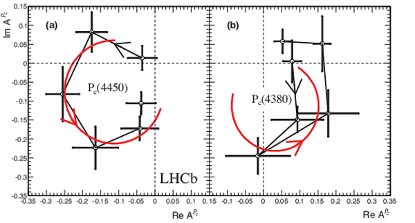
Fitted values of the real and imaginary parts of the amplitudes for the baseline ($3/2^-$, $5/2^+$) fit for a) the $P_c(4450)^+$ state and b) the $P_c(4380)^+$ state, each divided into six $m_{ { J \mskip -3mu/\mskip -2mu\psi \mskip 2mu} p}$ bins of equal width between $-\Gamma_0$ and $+\Gamma_0$ shown in the Argand diagrams as connected points with error bars ($m_{ { J \mskip -3mu/\mskip -2mu\psi \mskip 2mu} p}$ increases counterclockwise). The solid (red) curves are the predictions from the Breit-Wigner formula for the same mass ranges with $M_0$ ($\Gamma_0$) of 4450 (39) $\mathrm{ Me V}$ and 4380 (205) $\mathrm{ Me V}$ , respectively, with the phases and magnitudes at the resonance masses set to the average values between the two points around $M_0$. The phase convention sets $B_{0,\frac{1}{2}}=(1,0)$ for $\Lambda (1520)$. Systematic uncertainties are not included.

(a) Invariant mass squared of $ { J \mskip -3mu/\mskip -2mu\psi \mskip 2mu} K^-$ versus $ { J \mskip -3mu/\mskip -2mu\psi \mskip 2mu} p$ and (b) of $ { J \mskip -3mu/\mskip -2mu\psi \mskip 2mu} K^-$ versus $K^-p$ for candidates within $\pm15$ MeV of the $\Lambda ^0_ b $ mass.

Projections onto $m_{ { J \mskip -3mu/\mskip -2mu\psi \mskip 2mu} K}$ in various intervals of $m_{Kp}$ for the reduced model fit (cFit) with two $P_c^+$ states of $J^P$ equal to $3/2^-$ and $5/2^+$: (a) $m_{Kp}<1.55$ GeV, (b) $1.55<m_{Kp}<1.70$ GeV, (c) $1.70<m_{Kp}<2.00$ GeV, (d) $m_{Kp}>2.00$ GeV, and (e) all $m_{Kp}$. The data are shown as (black) squares with error bars, while the (red) circles show the results of the fit. The individual resonances are given in the legend.

Various decay angular distributions for the fit with two $P_c^+$ states for $m(K^-p)>2$ GeV. The data are shown as (black) squares, while the (red) circles show the results of the fit. Each fit component is also shown. The angles are defined in the text.

Results of the fit with one $J^P=5/2^+$ $P_c^+$ candidate. (a) Projection of the invariant mass of $K^-p$ combinations from $\Lambda ^0_ b \rightarrow { J \mskip -3mu/\mskip -2mu\psi \mskip 2mu} K^-p$ candidates. The data are shown as (black) squares with error bars, while the (red) circles show the results of the fit; (b) the corresponding $ { J \mskip -3mu/\mskip -2mu\psi \mskip 2mu} p$ mass projection. The (blue) shaded plot shows the $P_c^+$ projection, the other curves represent individual $\Lambda ^*$ states.

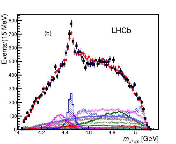
Results from cFit for (a) $m_{Kp}$ and (b) $m_{ { J \mskip -3mu/\mskip -2mu\psi \mskip 2mu} p}$ for the extended model with two $P_c^+$ states. The data are shown (black) squares with error bars, while the (red) circles show the results of the fit. Each $\Lambda ^*$ component is also shown. The (blue) open squares and (purple) solid squares show the two $P_c^+$ states.

Coordinate axes for the spin quantization of particle $A$ (bottom part), chosen to be the helicity frame of $A$ ($\hat{z}_{0}||\vec{p}_{A}$ in the rest frame of its mother particle or in the laboratory frame), together with the polar ($\BA{\theta}{B}{A}$) and azimuthal ($\BA{\phi}{B}{A}$) angles of the momentum of its daughter $B$ in the $A$ rest frame (top part). Notice that the directions of these coordinate axes, denoted as $\BA{\hat{x}}{0}{A}$, $\BA{\hat{y}}{0}{A}$, and $\BA{\hat{z}}{0}{A}$, do not change when boosting from the helicity frame of $A$ to its rest frame. After the Euler rotation ${\cal R}(\alpha=\BA{\phi}{B}{A},\beta=\BA{\theta}{B}{A},\gamma=0)$ (see the text), the rotated $z$ axis, $\BA{\hat{z}}{2}{A}$, is aligned with the $B$ momentum; thus the rotated coordinates become the helicity frame of $B$. If $B$ has a sequential decay, then the same boost-rotation process is repeated to define the helicity frame for its daughters.

Definition of the decay angles in the $\Lambda ^*$ decay chain.

Definition of the decay angles in the $P_c^+$ decay chain.

Definition of the $\theta_p$ angle.

Parameterized dependence of (a) the relative signal efficiency and of (b) the background density on the Dalitz plane. The units of the relative efficiency and of the relative background density are arbitrary.

Animated gif made out of all figures.

The $\Lambda ^*$ resonances used in the different fits. Parameters are taken from the PDG [14]. We take $5/2^-$ for the $J^P$ of the $\Lambda (2585)$. The number of $LS$ couplings is also listed for both the "reduced" and "extended" models. To fix overall phase and magnitude conventions, which otherwise are arbitrary, we set $B_{0,\frac{1}{2}}=(1,0)$ for $\Lambda (1520)$. A zero entry means the state is excluded from the fit.

Summary of systematic uncertainties on $P_c^+$ masses, widths and fit fractions, and $\Lambda ^*$ fit fractions. A fit fraction is the ratio of the phase space integrals of the matrix element squared for a single resonance and for the total amplitude. The terms "low" and "high" correspond to the lower and higher mass $P_c^+$ states. The sFit/cFit difference is listed as a cross-check and not included as an uncertainty.

Fit fractions of the different components from cFit and sFit for the default ($3/2^-$, $5/2^+$) model. Uncertainties are statistical only.