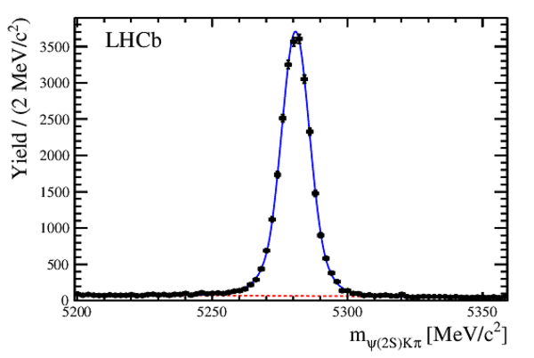
Spectrum of the $\psi {(2S)} K \pi$ system invariant mass. Black dots are the data, the continuous (blue) line represents the fit result and the dashed (red) line represents the background component.

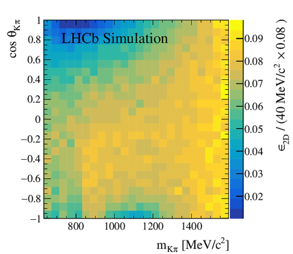
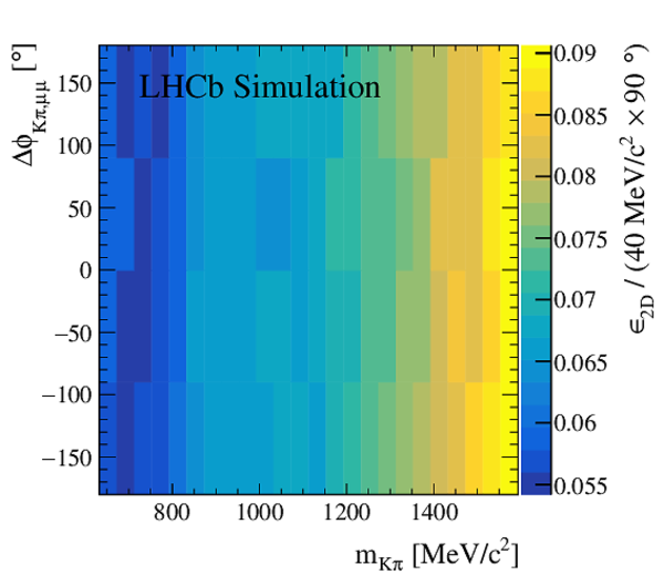
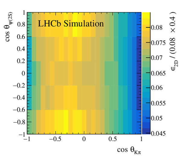
The 2D efficiency shown in the following planes: (top-left) ($ m _{ K \pi} $,$\cos\theta_{K^{*0}}$), (top-middle) ($ m _{ K \pi} $,$ \mathrm{\Delta\phi_{\it{ K }\pi,\mu\mu}} $), (top-right) ($ m _{ K \pi} $,$\mathrm{cos{\theta}_{\psi {(2S)} }} $), (bottom-left) ($\cos\theta_{K^{*0}}$,$\mathrm{cos{\theta}_{\psi {(2S)} }} $), (bottom-middle) ($\cos\theta_{K^{*0}}$,$ \mathrm{\Delta\phi_{\it{ K }\pi,\mu\mu}} $), (bottom-right) ($\mathrm{cos{\theta}_{\psi {(2S)} }} $,$ \mathrm{\Delta\phi_{\it{ K }\pi,\mu\mu}} $). Corrections for the efficiency are applied in the 4D space; the 2D plots allow visualization of their behavior.

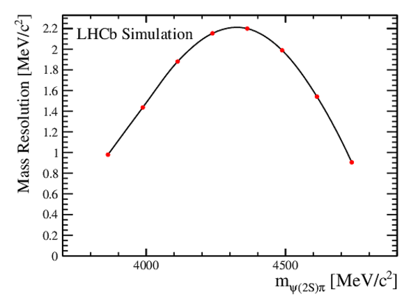
The $\psi {(2S)} \pi$ invariant mass resolution as determined from simulated data (red dots). The continuous line is a spline-based interpolation.

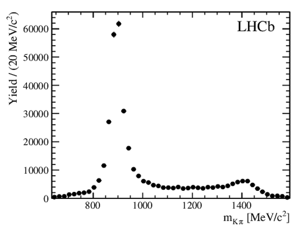
Distributions of (left) $ m _{ K \pi}$ and (right) $\cos\theta_{K^{*0}}$, after background subtraction and efficiency correction.

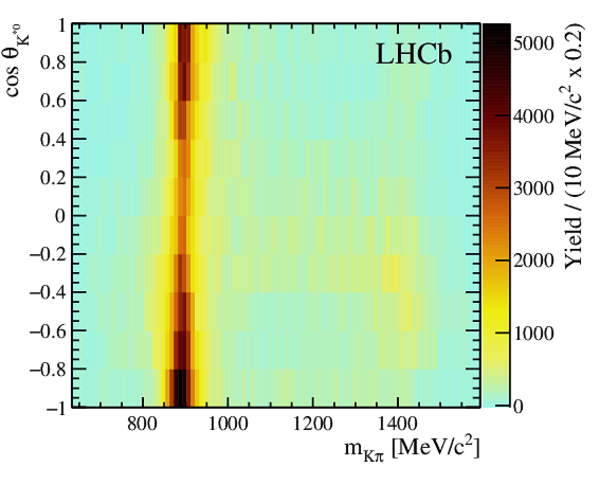
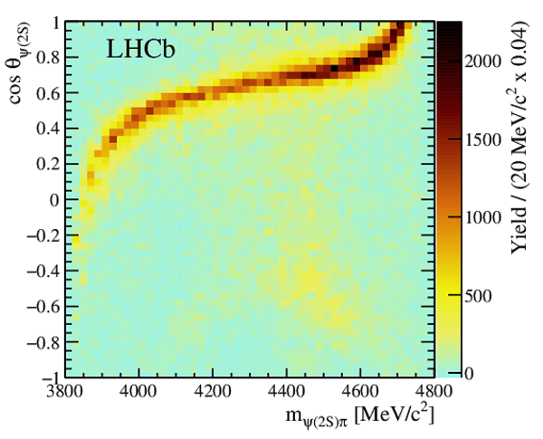
The two-dimensional distributions ( $ m _{ K \pi}$ ,$\cos\theta_{K^{*0}}$) and ($m_{\psi {(2S)} \pi}$,$\mathrm{cos{\theta}_{\psi {(2S)} }} $) are shown in the left and the right plots, respectively, after background subtraction and efficiency correction.

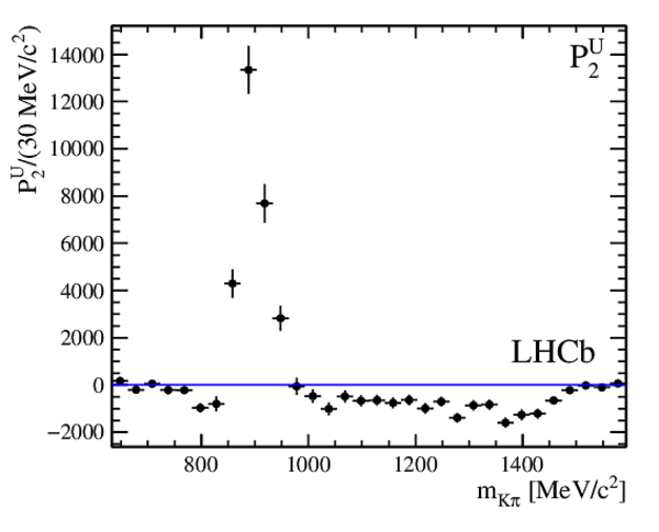
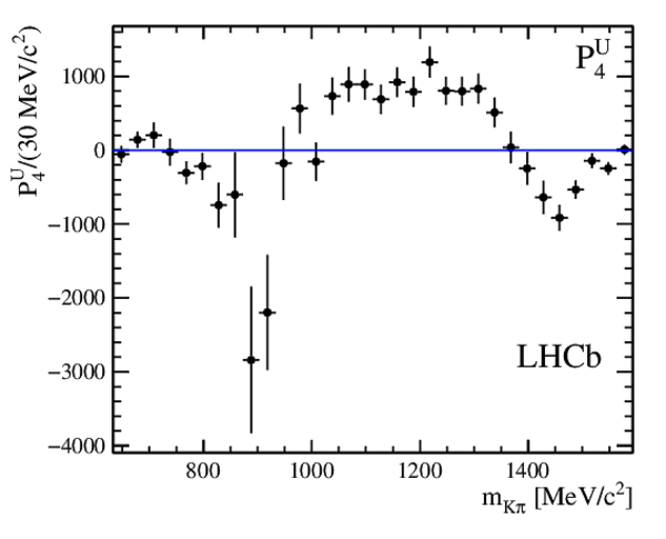
Dependence on $ m _{ K \pi}$ of the first six $ K \pi $ moments of the $ B ^0 \rightarrow \psi {(2S)} K ^+ \pi ^- $ decay mode as determined from data.

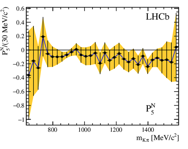
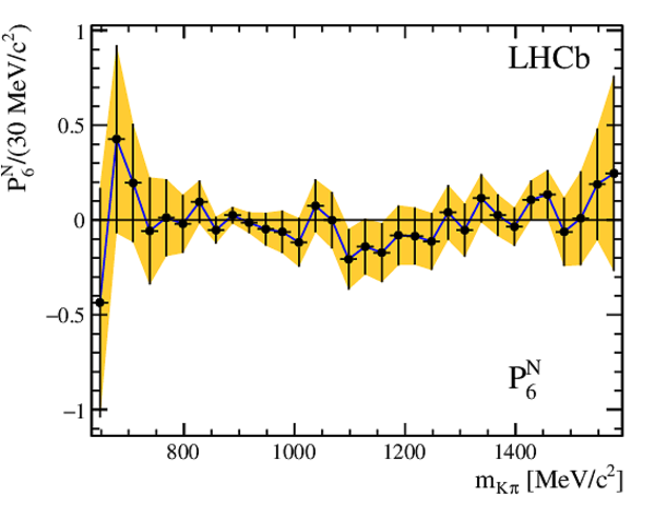
First six normalized $ K \pi $ moments of the $ B ^0 \rightarrow \psi {(2S)} K ^+ \pi ^- $ decay mode as a function of $ m _{ K \pi}$ . The shaded (yellow) bands indicate the $\pm 1\sigma$ variations of the moments.

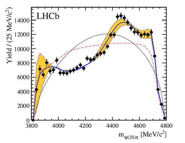
Background subtracted and efficiency corrected spectrum of $m_{\psi {(2S)} \pi}$. Black points represent data. Superimposed are the distributions of the Monte Carlo simulation: the dotted (black) line corresponds to the pure phase-space case; in the dash-dotted (red) line the $ m _{ K \pi}$ spectrum is weighted to reproduce the experimental distribution; in the continuous (blue) line the angular structure of the $ K \pi $ system is incorporated using Legendre polynomials up to (left) $ l_{\text{max}} =4$ and (right) $ l_{\text{max}} =6$. The shaded (yellow) bands are related to the uncertainty on normalized moments, which is due to the statistical uncertainty that comes from the data. Therefore the two uncertainties should not be combined when comparing data and Monte Carlo predictions. See text for further details.

The experimental spectrum of $m_{\psi {(2S)} \pi}$ is shown by the black points. Superimposed are the distributions of the Monte Carlo simulation: the dotted(black) line corresponds to the pure phase-space case; in the dash-dotted (red) line the $ m _{ K \pi}$ spectrum is weighted to reproduce the experimental distribution; in the continuous (blue) line the angular structure of the $ K \pi $ system is incorporated using Legendre polynomials with index $ l_{\text{max}} $ variable according to $ m _{ K \pi}$ as described in \autoref{eq:slices}, reaching up to $ l_{\text{max}} =4$. The shaded (yellow) bands are related to the uncertainty on normalized moments, which is due to the statistical uncertainty that comes from the data. Therefore the two uncertainties should not be combined when comparing data and Monte Carlo predictions. See text for further details.

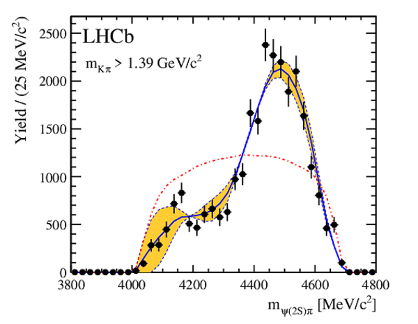
Black points represent the experimental distributions of $m_{\psi {(2S)} \pi}$ for the indicated $ m _{ K \pi}$ intervals. The dash-dotted (red) line is obtained by modifying the $ m _{ K \pi}$ spectrum of the phase-space simulation according to the $ m _{ K \pi}$ experimental spectrum. In the continuous (blue) line the angular structure of the $ K \pi $ system is incorporated using Legendre polynomials with variable index $ l_{\text{max}} $ according to \autoref{eq:slices}. The shaded (yellow) bands are related to the uncertainty on normalized moments, which is due to the statistical uncertainty that comes from the data. Therefore the two uncertainties should not be combined when comparing data and Monte Carlo predictions. See text for further details.

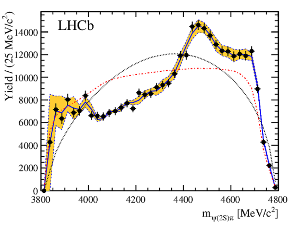
The experimental spectrum of $m_{\psi {(2S)} \pi}$ is shown by the black points. Superimposed are the distributions of the Monte Carlo simulation: the dotted (black) line corresponds to the pure phase space case; in the dash-dotted (red) line the $ m _{ K \pi}$ spectrum is weighted to reproduce the experimental distribution; in the continuous (blue) line the angular structure of the $ K \pi $ system is incorporated using Legendre polynomials up to $ l_{\text{max}} =30$ which implies a full description of the spectrum features even if it corresponds to an unphysical configuration of the $ K \pi $ system. The shaded (yellow) bands are related to the uncertainty on normalized moments.

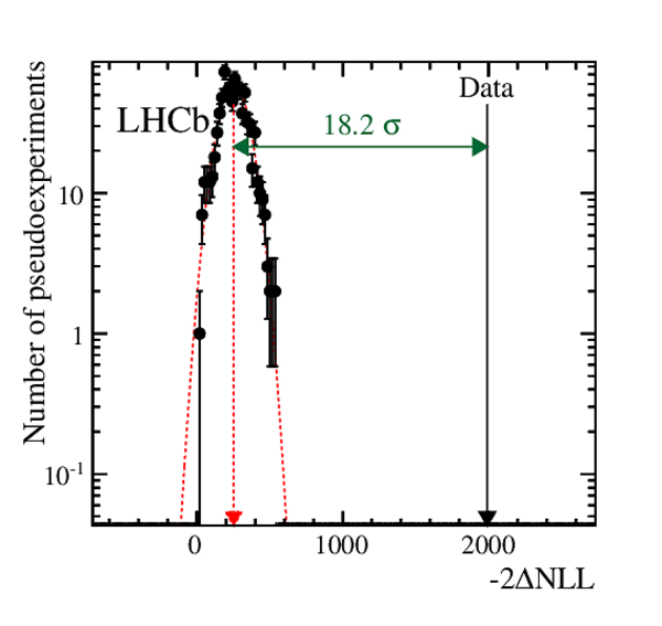
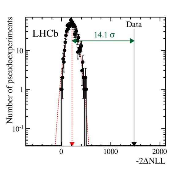
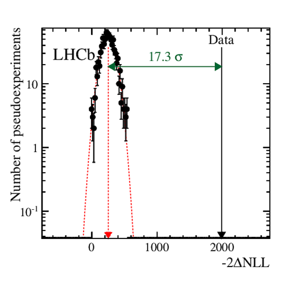
Distributions of $-2\Delta\textrm{NLL}$ for the pseudoexperiments (black dots), fitted with a Gaussian function (dashed red line), in three different configurations of the $ K \pi $ system angular contributions: (left) $ l_{\text{max}} =4$, (middle) $ l_{\text{max}} =6$ and (right) $ l_{\text{max}} $ variable according to \autoref{eq:slices}. The black arrow represents the $-2\Delta\textrm{NLL}$ value obtained on data.

Distributions of $-2\Delta\textrm{NLL}$ for the pseudoexperiments (black dots), fitted with a Gaussian function (dashed red line), for the region $1000 {\mathrm{ Me V /}c^2} < m _{ K \pi} <1390 {\mathrm{ Me V /}c^2} $ in three different configurations of the $ K \pi $ system angular contributions: (left) $ l_{\text{max}} =4$, (middle) $ l_{\text{max}} =6$ and (right) $ l_{\text{max}} $ variable according to \autoref{eq:slices}. The black arrow represents the $-2\Delta\textrm{NLL}$ value obtained on data.

Animated gif made out of all figures.

Results of the fit to the invariant mass spectrum of the $\psi {(2S)} K \pi$ system. The signal and the background yields are calculated in the signal region defined by the interval of $\pm 2\sigma_{ B ^0 }$ around $M_{ B ^0 }$.

Experimental resolution of kinematical quantities, as estimated from Monte Carlo simulations.

Mass, width, spin and parity of resonances known to decay to the $ K \pi $ final state [5]. The list is limited to masses up to just above the maximum invariant mass for the $ K \pi $ system which, in the decay $ B ^0 \rightarrow \psi {(2S)} K ^+ \pi ^- $, is $1593 {\mathrm{ Me V /}c^2} $.

Significance, {\it S}, in units of standard deviations, at which the hypothesis that $m_{\psi {(2S)} \pi}$ data can be described as a reflection of the $ K \pi $ system angular structure is excluded, for different configurations of the $ K \pi $ system angular contributions. In the second column the whole $ m _{ K \pi} $ spectrum has been analyzed while in the third one the specified $ m _{ K \pi} $ cut is applied.