Angular analysis of the $B^{0}\rightarrow K^{*0}\mu^{+}\mu^{-}$ decay using 3 fb$^{-1}$ of integrated luminosity
[to restricted-access page]Information
LHCb-PAPER-2015-051
CERN-PH-EP-2015-314
arXiv:1512.04442 [PDF]
(Submitted on 14 Dec 2015)
JHEP 02 (2016) 104
Inspire 1409497
Tools
Abstract
An angular analysis of the $B^{0}\rightarrow K^{*0}(\rightarrow K^{+}\pi^{-})\mu^{+}\mu^{-}$ decay is presented. The dataset corresponds to an integrated luminosity of $3.0 { fb^{-1}}$ of $pp$ collision data collected at the LHCb experiment. The complete angular information from the decay is used to determine $C P$-averaged observables and $C P$ asymmetries, taking account of possible contamination from decays with the $K^{+}\pi^{-}$ system in an S-wave configuration. The angular observables and their correlations are reported in bins of $q^2$, the invariant mass squared of the dimuon system. The observables are determined both from an unbinned maximum likelihood fit and by using the principal moments of the angular distribution. In addition, by fitting for $q^2$-dependent decay amplitudes in the region $1.1<q^{2}<6.0\mathrm{ Ge V}^{2}/c^{4}$, the zero-crossing points of several angular observables are computed. A global fit is performed to the complete set of $C P$-averaged observables obtained from the maximum likelihood fit. This fit indicates differences with predictions based on the Standard Model at the level of 3.4 standard deviations. These differences could be explained by contributions from physics beyond the Standard Model, or by an unexpectedly large hadronic effect that is not accounted for in the Standard Model predictions.
Figures and captions
|
Invariant mass of the $ K ^+ \pi ^- \mu ^+\mu ^- $ system versus $q^2$. The decay $ B ^0 \rightarrow K ^{*0} \mu ^+\mu ^- $ is clearly visible inside the dashed vertical lines. The horizontal lines denote the charmonium regions, where the tree-level decays $ B ^0 \rightarrow { J \mskip -3mu/\mskip -2mu\psi \mskip 2mu} K ^{*0} $ and $ B ^0 \rightarrow \psi {(2S)} K ^{*0} $ dominate. These candidates are excluded from the analysis. |
Fig1.pdf [30 KiB] HiDef png [704 KiB] Thumbnail [603 KiB] *.C file |

|
|
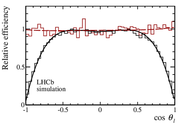
Relative efficiency in $\cos\theta_{l} $, $\cos\theta_{K} $, $\phi$ and $ q^2$ , as determined from a principal moment analysis of simulated three-body $ B ^0 \rightarrow K ^{*0} \mu ^+\mu ^- $ phase-space decays. The efficiency as a function of $\cos\theta_{l} $, $\cos\theta_{K} $ and $\phi$ is shown for the regions $0.1 < q^2 < 0.98\mathrm{ Ge V} ^{2}/c^{4}$ (black solid line) and $18.0 < q^2 <19.0 \mathrm{ Ge V} ^{2}/c^{4}$ (red dashed line). The efficiency as a function of $ q^2$ is shown after integrating over the decay angles. The histograms indicate the distribution of the simulated three-body $ B ^0 \rightarrow K ^{*0} \mu ^+\mu ^- $ phase-space decays used to determine the acceptance. |
effctl.pdf [16 KiB] HiDef png [135 KiB] Thumbnail [122 KiB] *.C file |
|
|
effctk.pdf [16 KiB] HiDef png [145 KiB] Thumbnail [129 KiB] *.C file |

|
|
|
effphi.pdf [21 KiB] HiDef png [131 KiB] Thumbnail [112 KiB] *.C file |

|
|
|
effqsq.pdf [18 KiB] HiDef png [77 KiB] Thumbnail [42 KiB] *.C file |

|
|
|
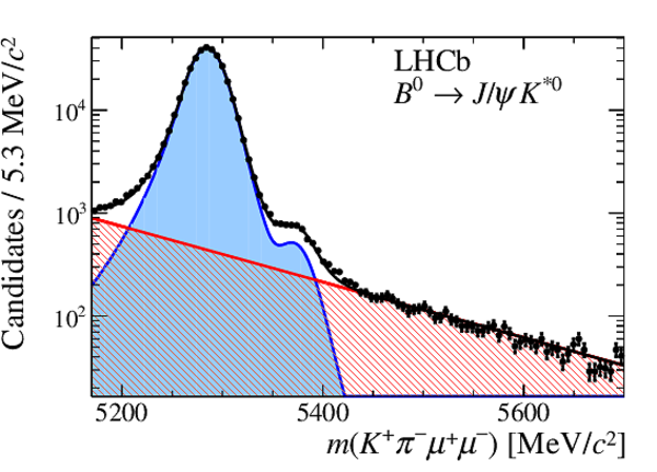
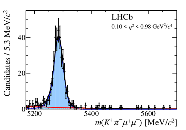
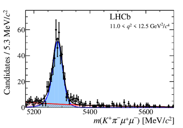
Invariant mass $m({ K ^+ \pi ^- \mu ^+\mu ^- })$ for (left) the control decay $ B ^0 \rightarrow { J \mskip -3mu/\mskip -2mu\psi \mskip 2mu} K ^{*0} $ and (right) the signal decay $ B ^0 \rightarrow K ^{*0} \mu ^+\mu ^- $, integrated over the full $q^2$ range (see text). Overlaid are the projections of the total fitted distribution (black line) and the signal and background components. The signal is shown by the blue shaded area and the background by the red hatched area. |
mjpsi.pdf [43 KiB] HiDef png [169 KiB] Thumbnail [133 KiB] *.C file |

|
|
msignal.pdf [43 KiB] HiDef png [230 KiB] Thumbnail [171 KiB] *.C file |

|
|
|
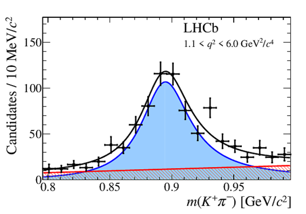
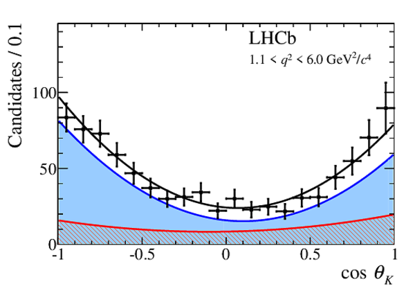
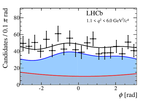
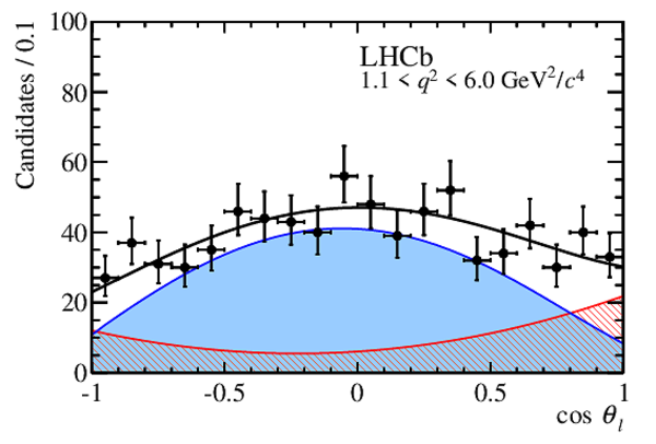
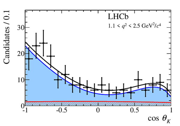
Angular and mass distributions for $1.1<q^2<6.0 {\mathrm{ Ge V^2 /}c^4} $. The distributions of $m( K ^+ \pi ^- )$ and the three decay angles are given for candidates in the signal mass window $\pm50 {\mathrm{ Me V /}c^2} $ around the known $ B ^0 $ mass. The candidates have been weighted to account for the acceptance. Overlaid are the projections of the total fitted distribution (black line) and its different components. The signal is shown by the blue shaded area and the background by the red hatched area. \vspace{2cm} |
m8.pdf [76 KiB] HiDef png [262 KiB] Thumbnail [199 KiB] *.C file |

|
|
mkpi8sig.pdf [20 KiB] HiDef png [284 KiB] Thumbnail [216 KiB] *.C file |
|
|
|
costhe[..].pdf [20 KiB] HiDef png [349 KiB] Thumbnail [247 KiB] *.C file |

|
|
|
costhe[..].pdf [20 KiB] HiDef png [282 KiB] Thumbnail [208 KiB] *.C file |
|
|
|
phi8sig.pdf [19 KiB] HiDef png [333 KiB] Thumbnail [245 KiB] *.C file |
|
|
|
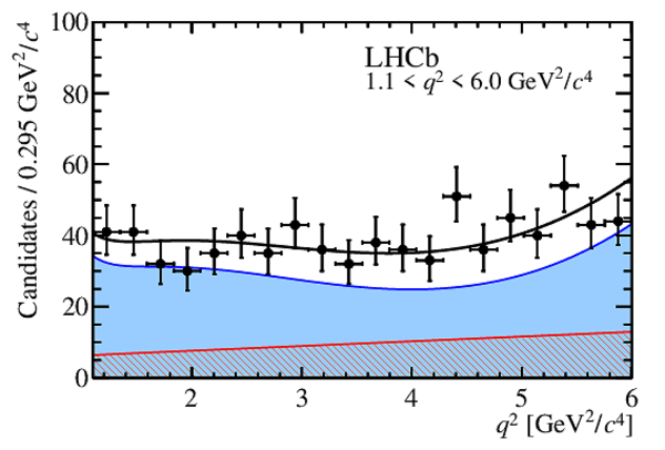
Angular and $ q^2$ distribution of candidates overlaid by the result of the amplitude fit. The distribution of candidates in $ q^2$ and the three decay angles is given in a $\pm50 {\mathrm{ Me V /}c^2} $ window around the known $ B ^0 $ mass. Overlaid are the projections of the total fitted distribution (black line) and its different components. The signal is shown by the blue shaded area and the background by the red hatched area. |
projec[..].pdf [17 KiB] HiDef png [306 KiB] Thumbnail [223 KiB] *.C file |
|
|
projec[..].pdf [17 KiB] HiDef png [312 KiB] Thumbnail [238 KiB] *.C file |

|
|
|
projec[..].pdf [17 KiB] HiDef png [282 KiB] Thumbnail [215 KiB] *.C file |

|
|
|
projec[..].pdf [17 KiB] HiDef png [314 KiB] Thumbnail [240 KiB] *.C file |
|
|
|
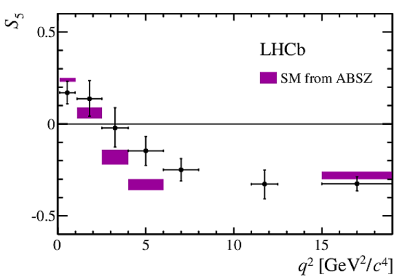
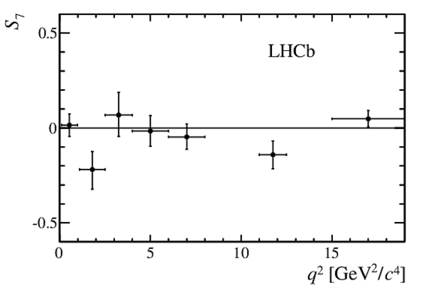
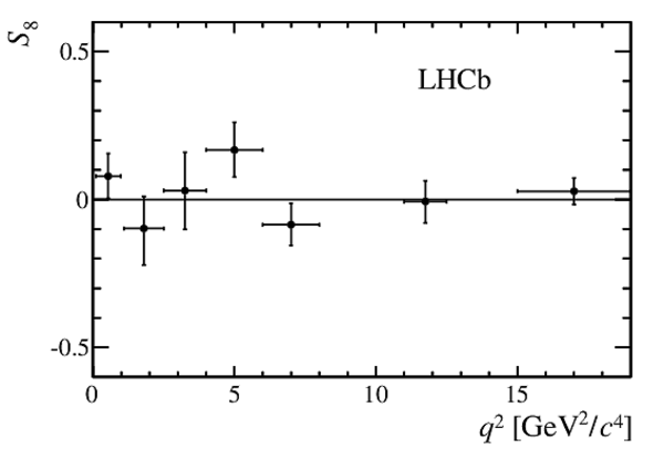
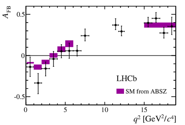
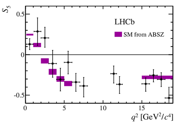
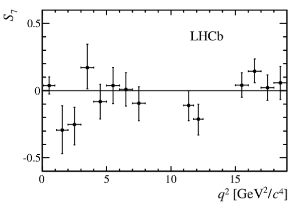
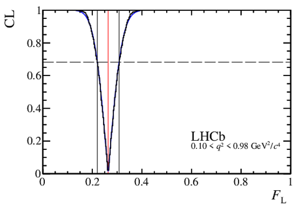
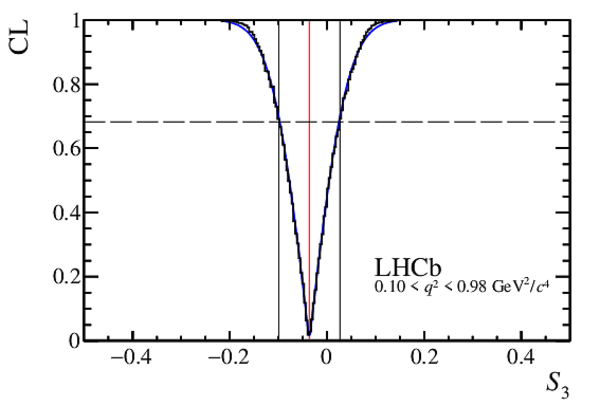
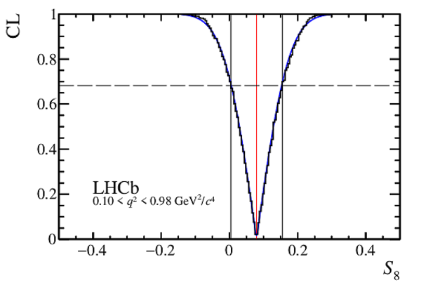
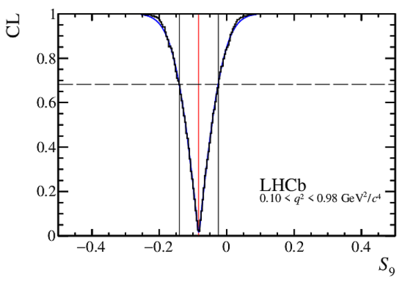
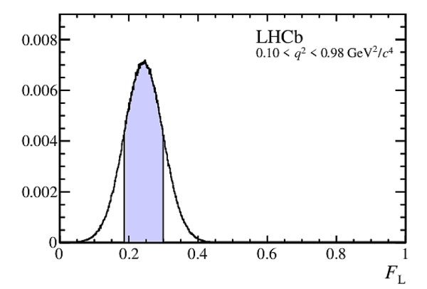
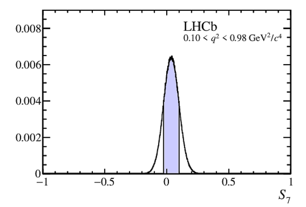
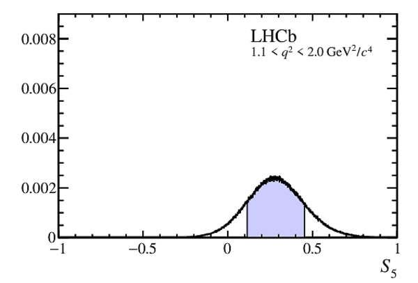
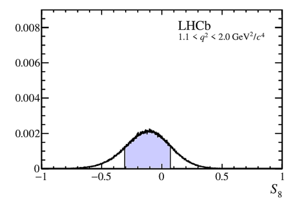
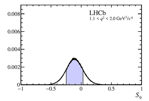
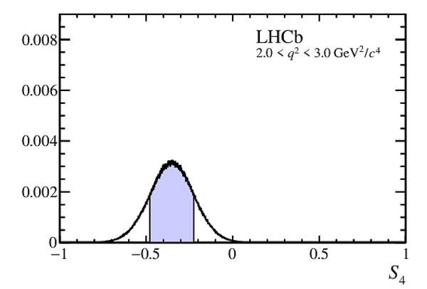
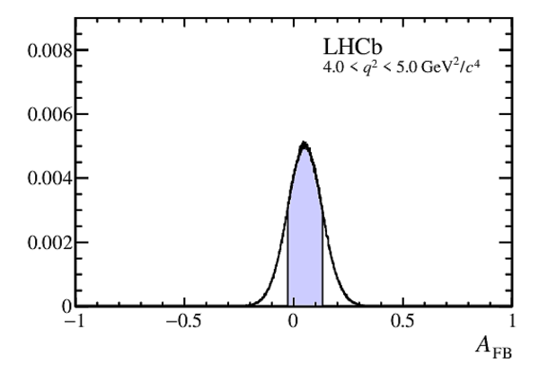
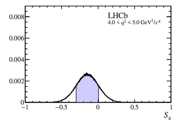
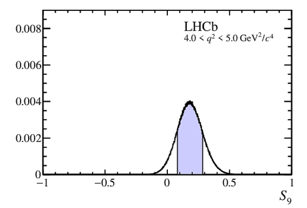
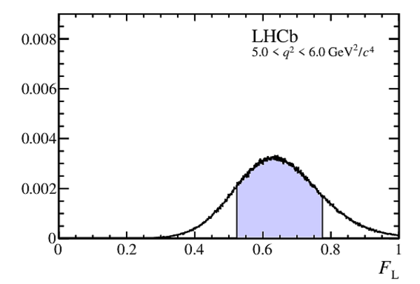
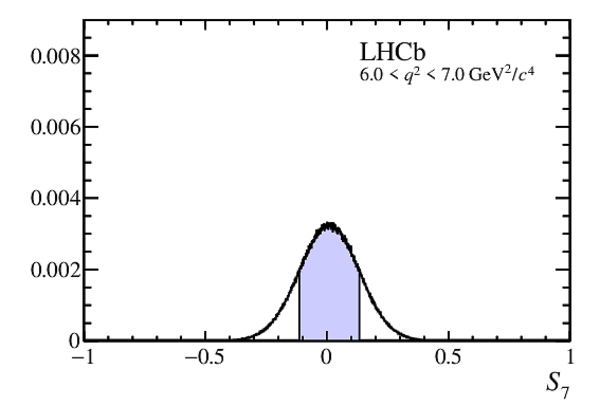
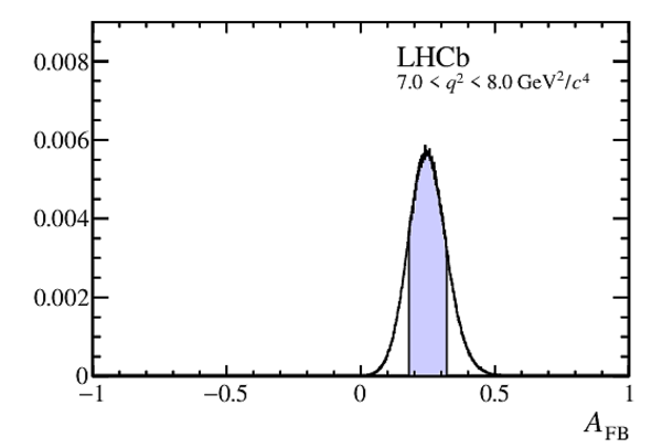
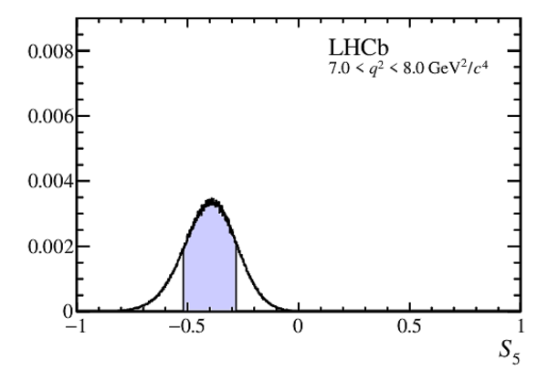
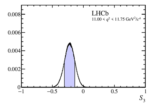
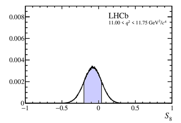
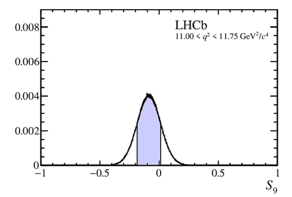
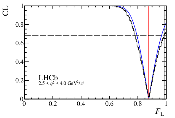
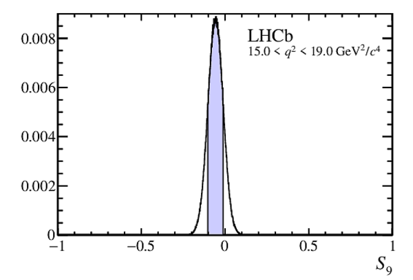
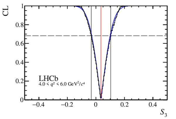
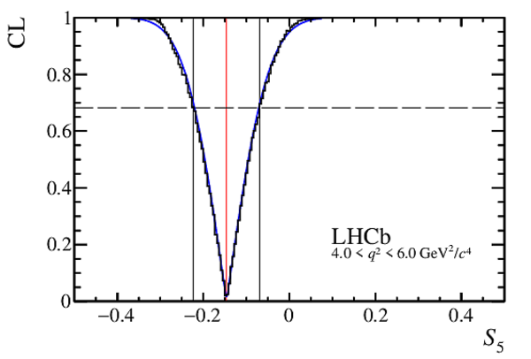
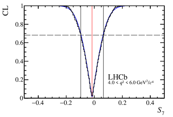
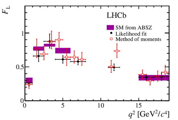
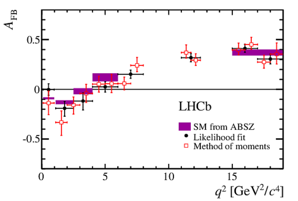
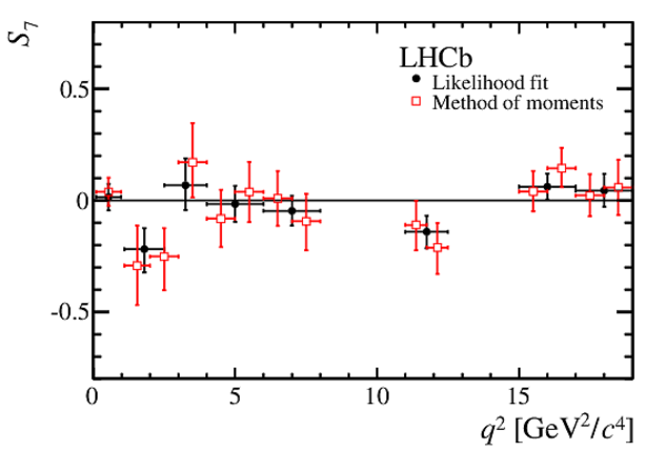
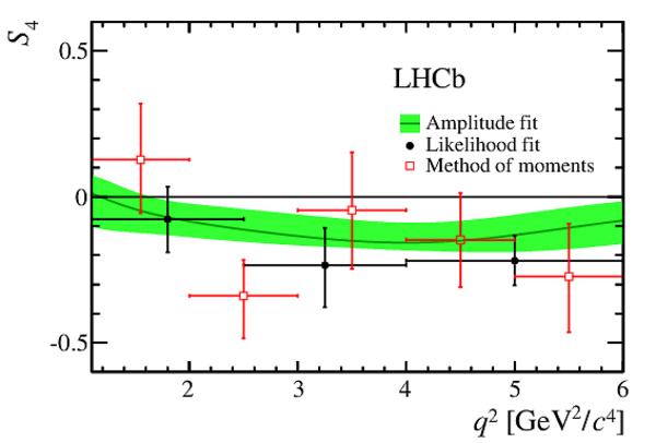
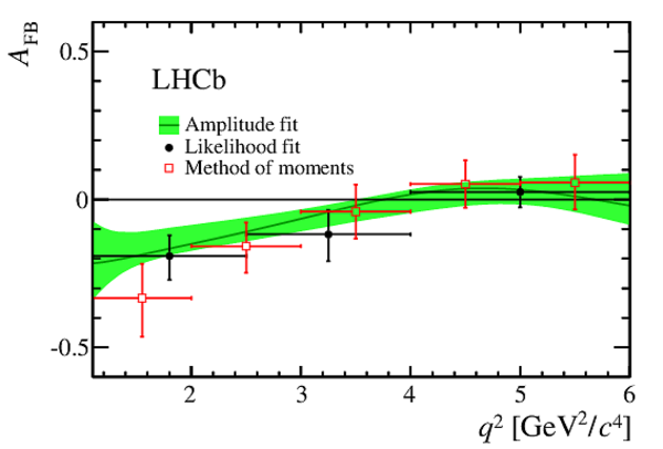
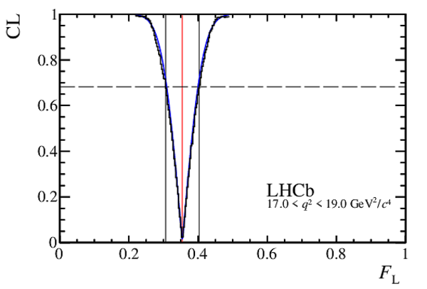
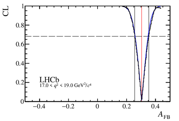
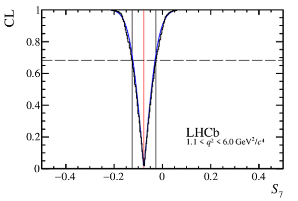
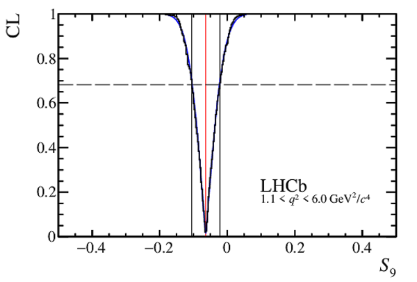
The $ C P$ -averaged observables in bins of $q^2$, determined from a maximum likelihood fit to the data. The shaded boxes show the SM predictions based on the prescription of Ref. [19]. |
FLPad.pdf [14 KiB] HiDef png [84 KiB] Thumbnail [80 KiB] *.C file |

|
|
AFBPad.pdf [14 KiB] HiDef png [78 KiB] Thumbnail [72 KiB] *.C file |
|
|
|
S3Pad.pdf [14 KiB] HiDef png [75 KiB] Thumbnail [70 KiB] *.C file |

|
|
|
S4Pad.pdf [14 KiB] HiDef png [77 KiB] Thumbnail [70 KiB] *.C file |
|
|
|
S5Pad.pdf [14 KiB] HiDef png [75 KiB] Thumbnail [71 KiB] *.C file |
|
|
|
S7Pad.pdf [13 KiB] HiDef png [46 KiB] Thumbnail [26 KiB] *.C file |
|
|
|
S8Pad.pdf [13 KiB] HiDef png [46 KiB] Thumbnail [26 KiB] *.C file |
|
|
|
S9Pad.pdf [13 KiB] HiDef png [46 KiB] Thumbnail [26 KiB] *.C file |

|
|
|
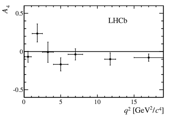
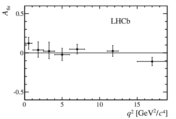
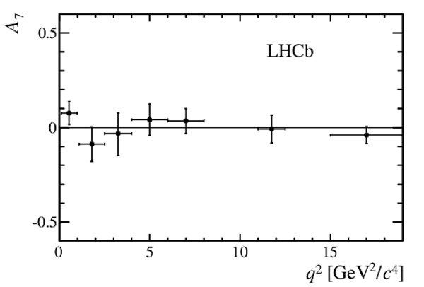
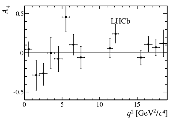
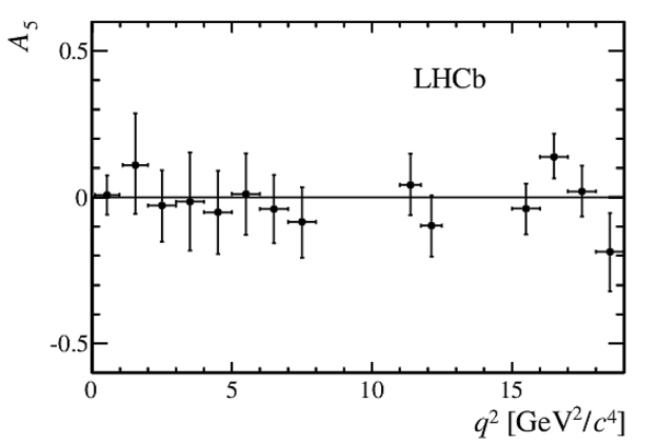
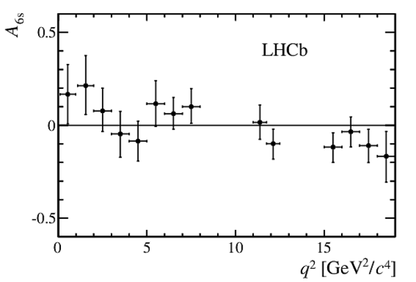
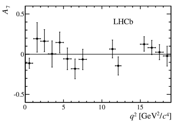
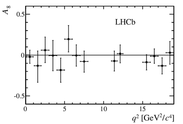
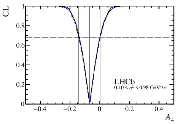
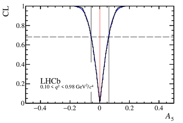
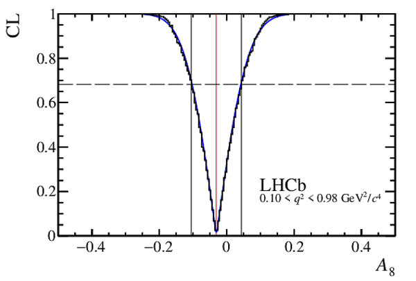
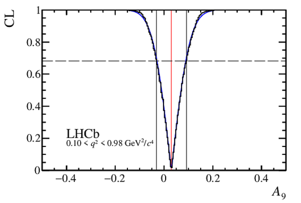
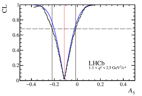
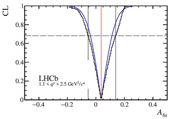
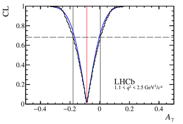
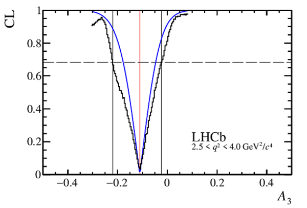
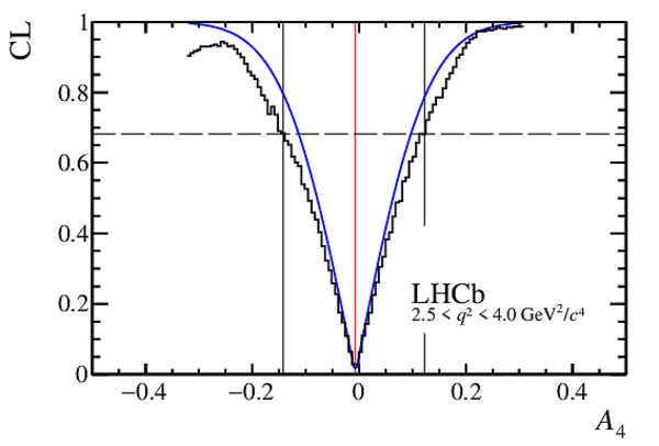
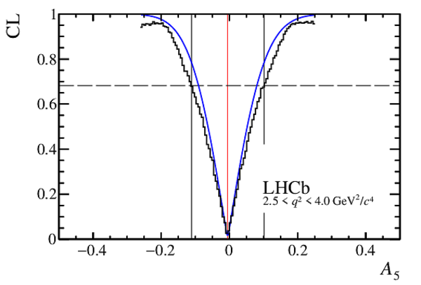
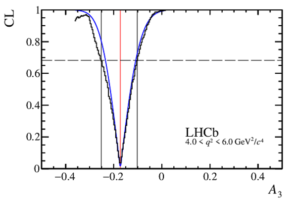
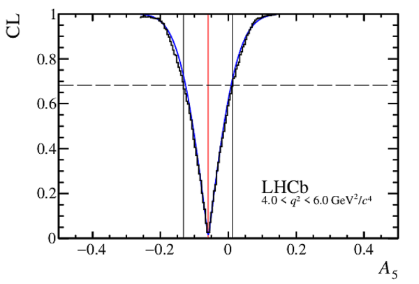
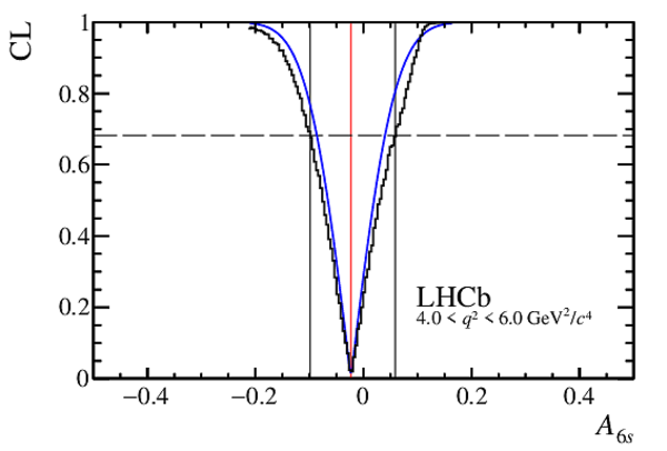
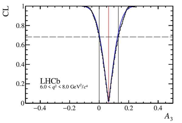
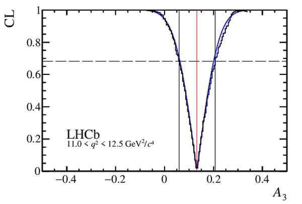
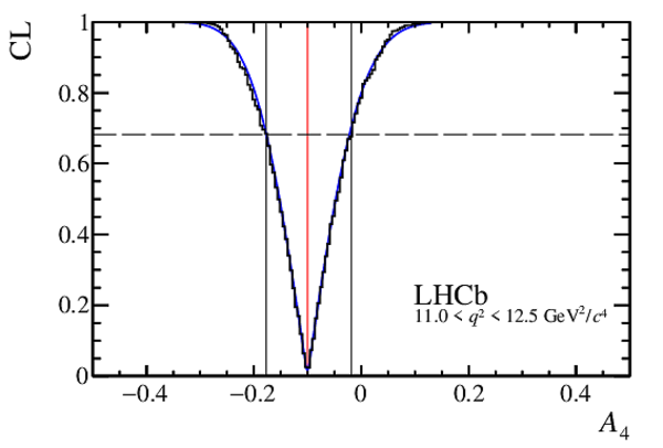
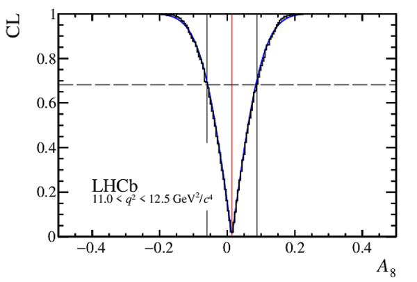
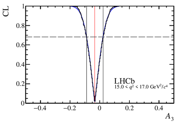
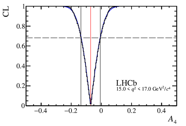
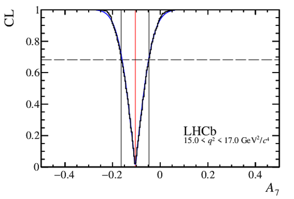
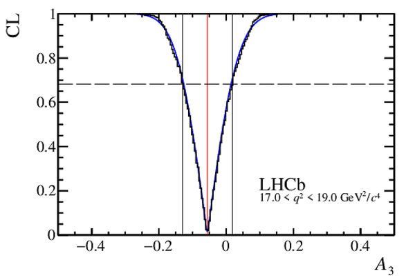
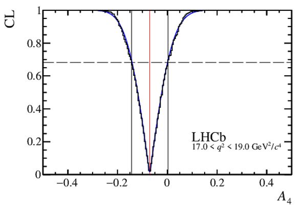
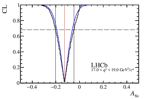
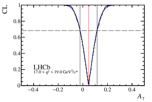
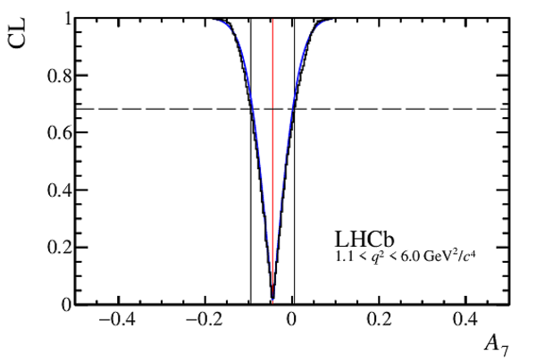
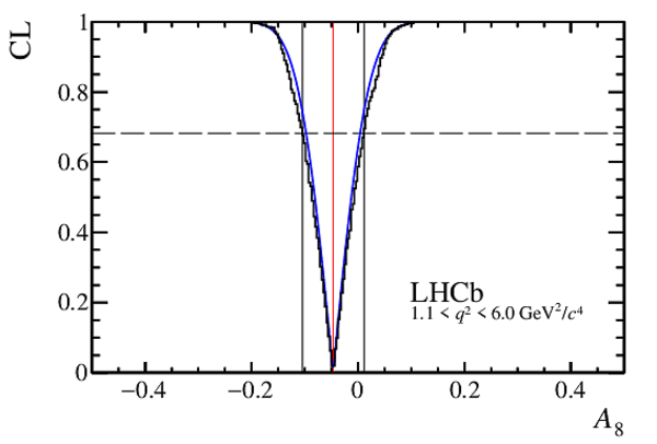
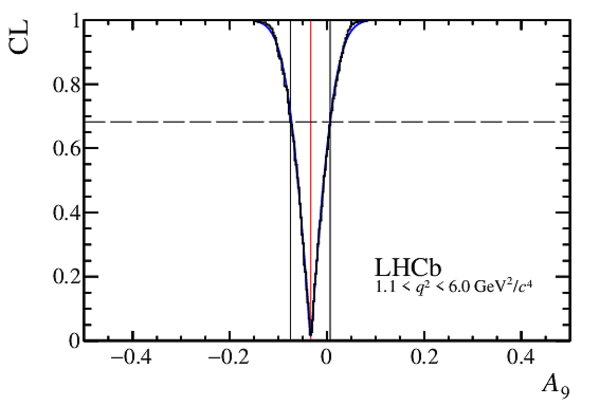
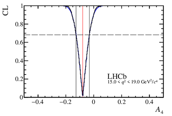
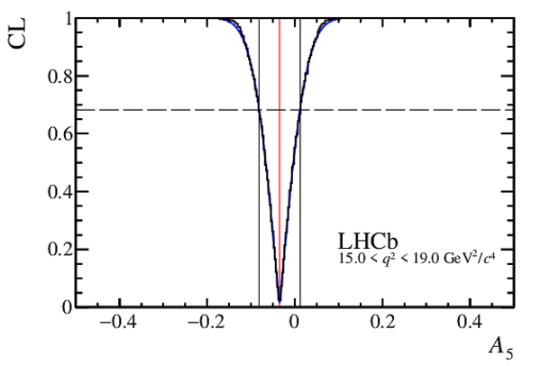
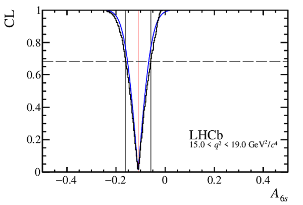
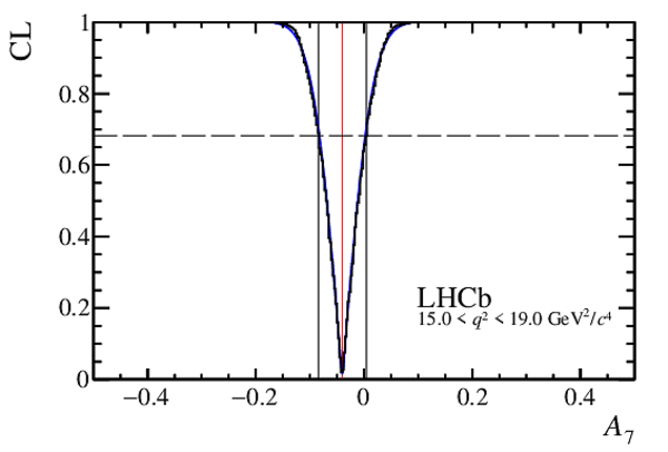
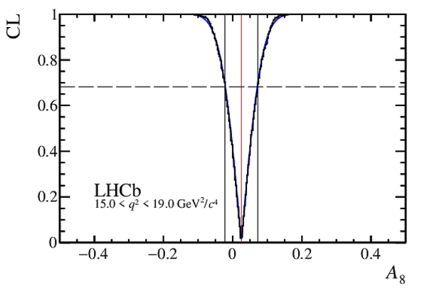
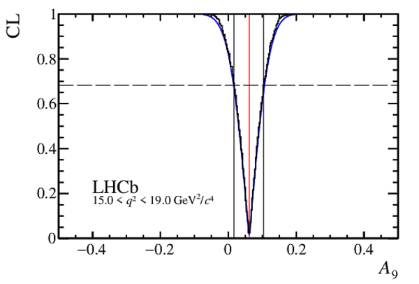
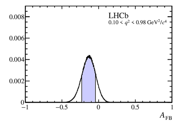
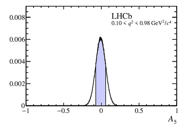
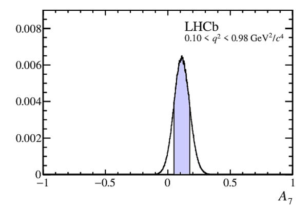
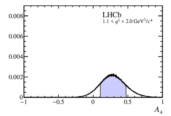
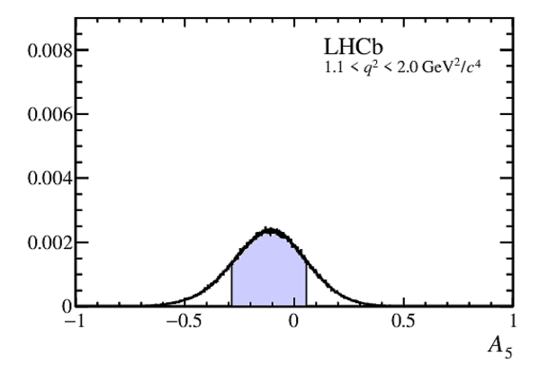
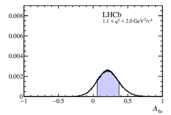
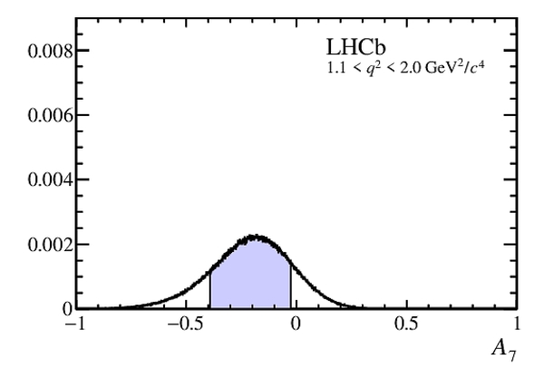
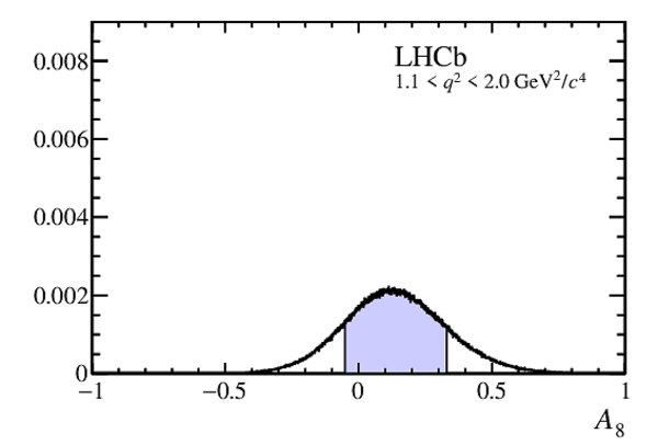
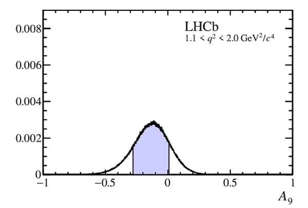
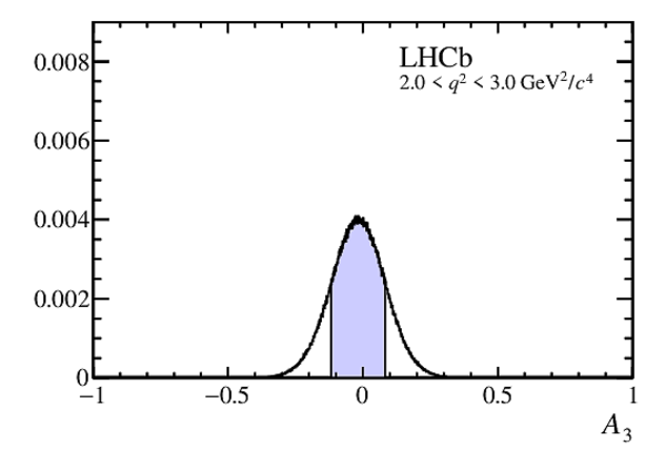
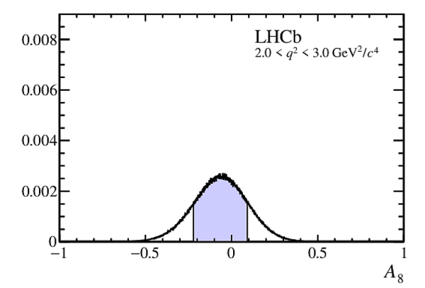
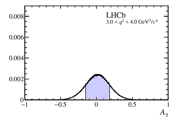
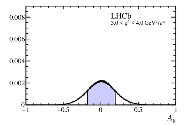
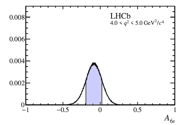
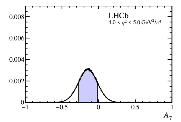
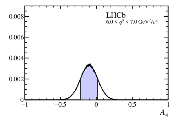
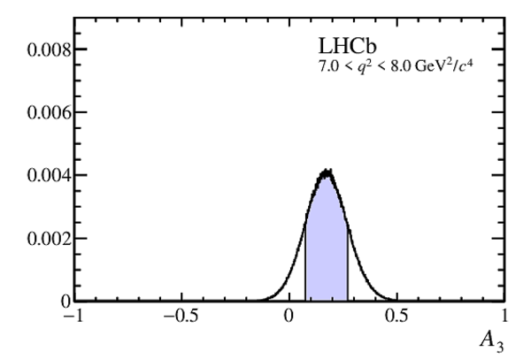
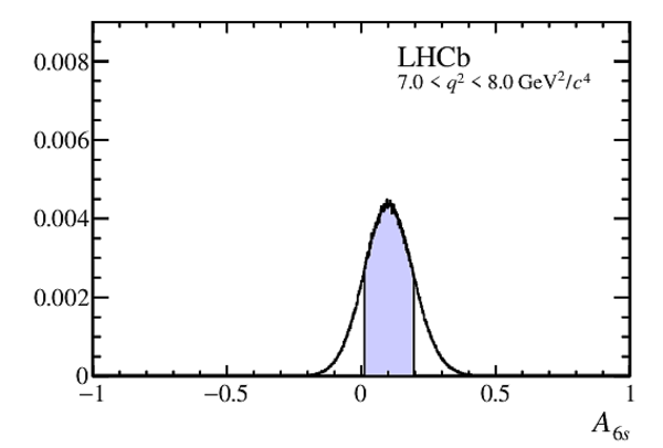
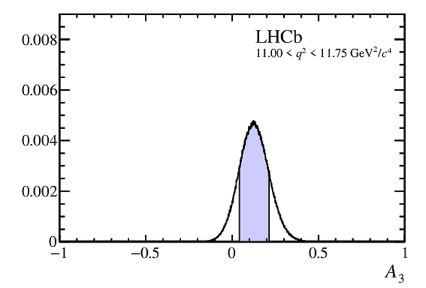
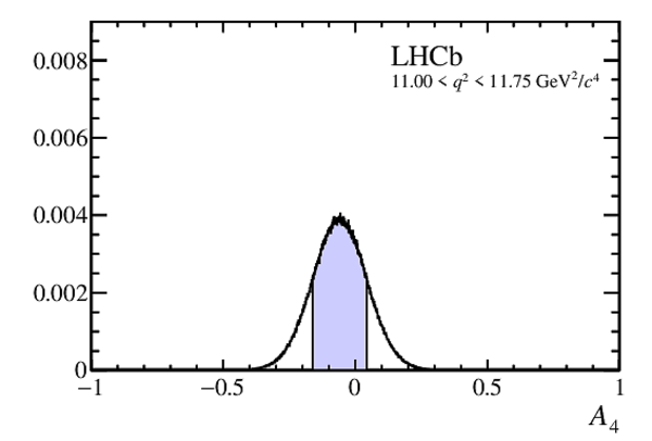
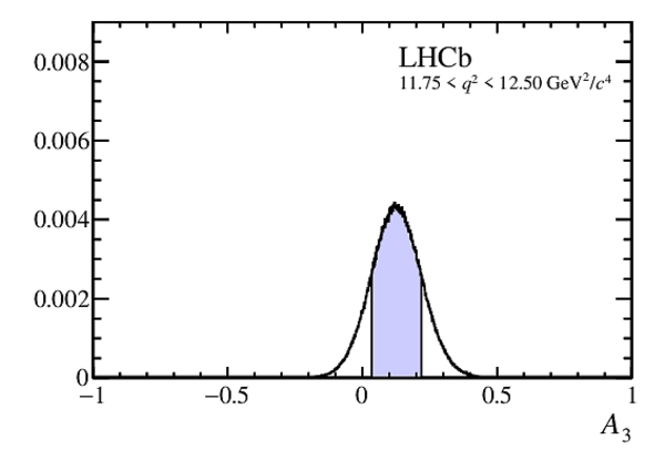
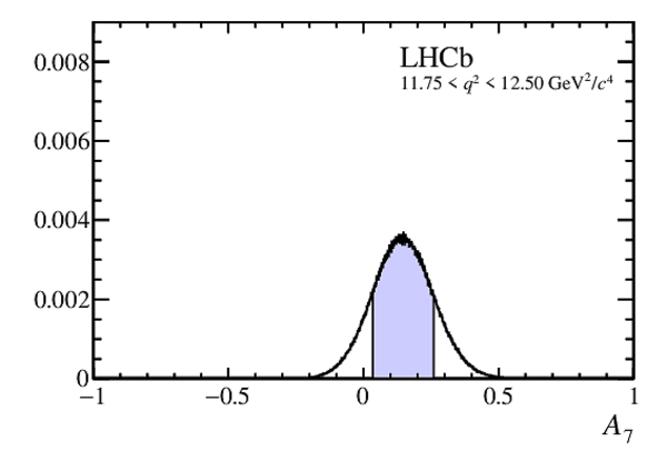
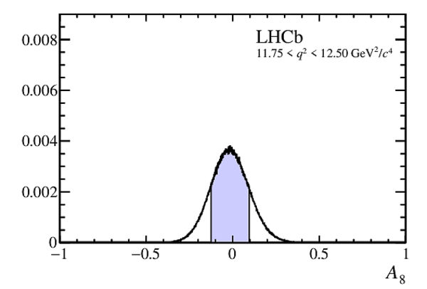
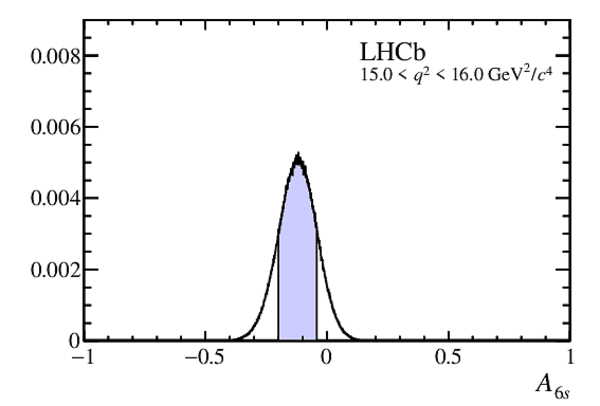
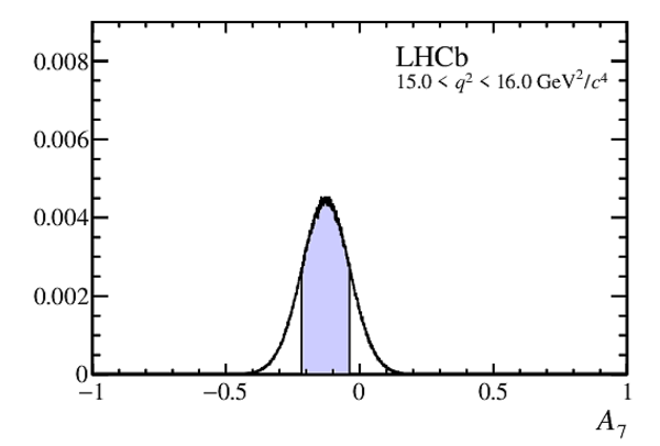
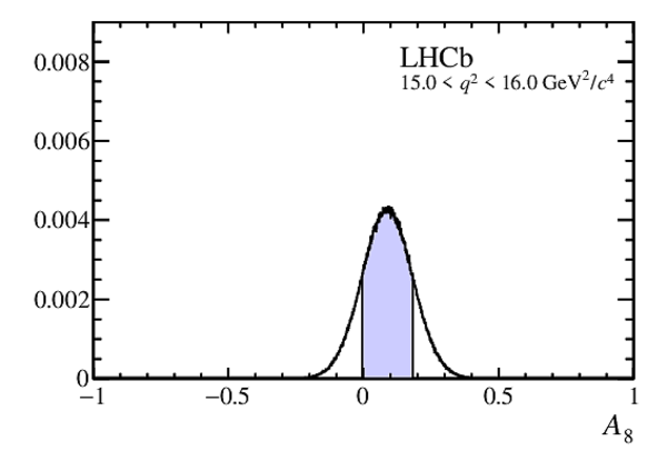
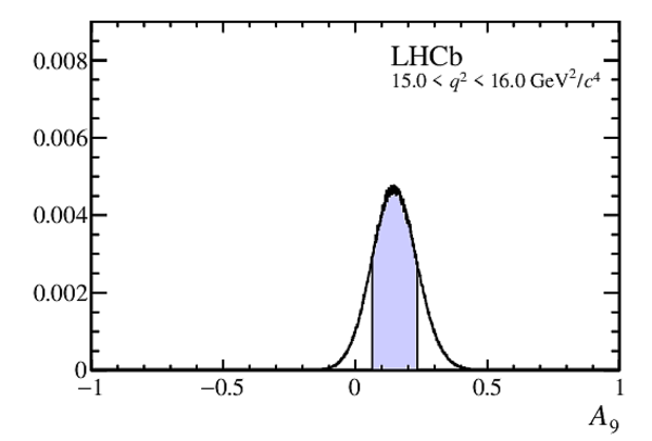
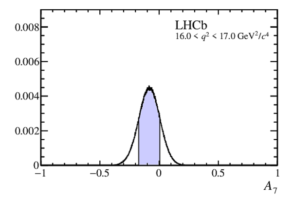
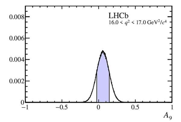
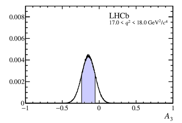
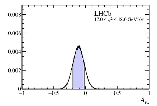
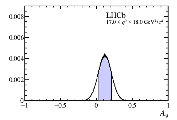
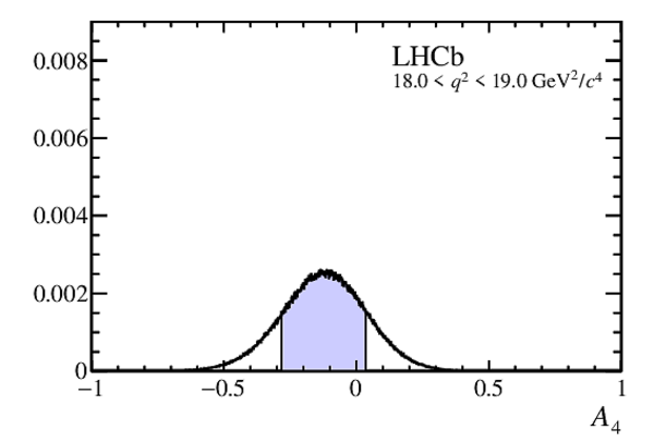
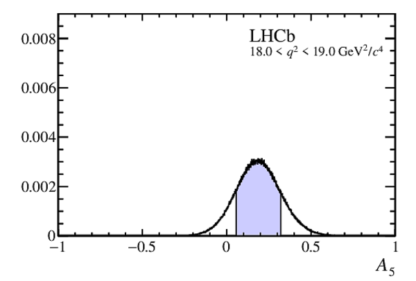
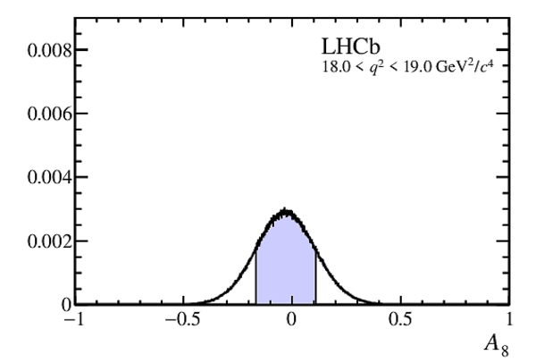
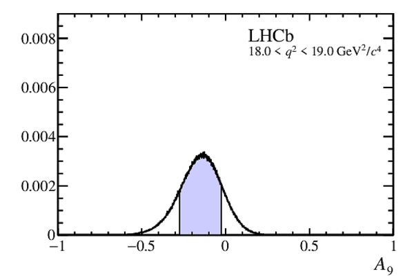
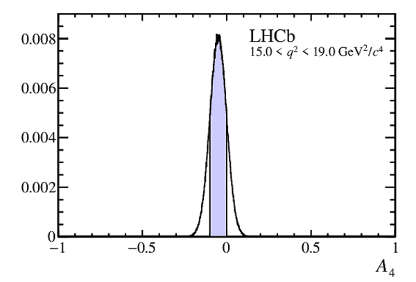
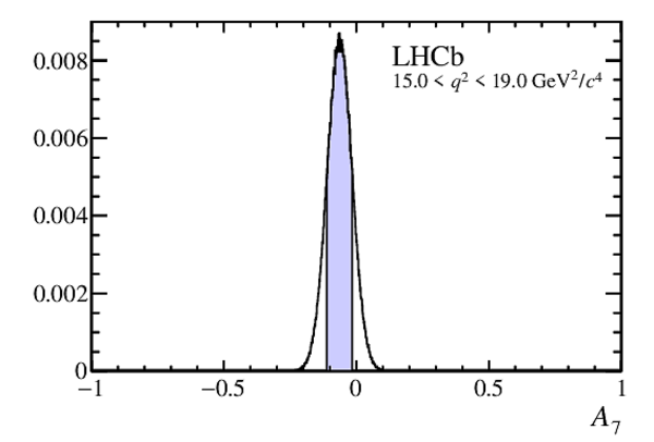
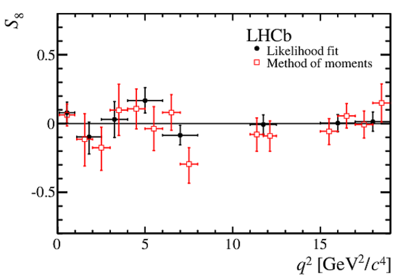
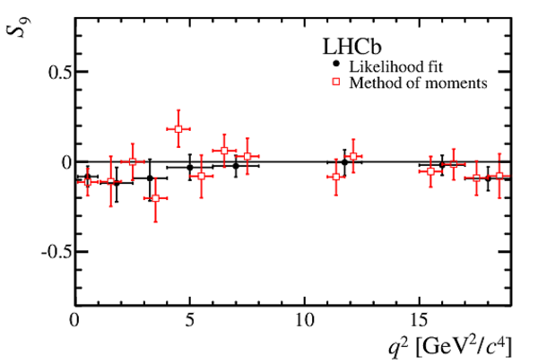
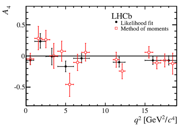
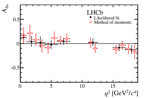
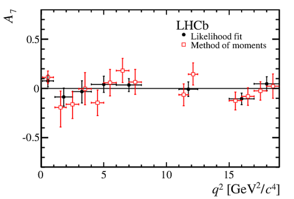
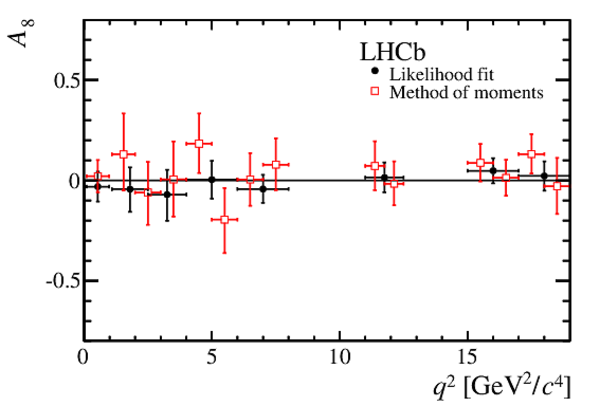
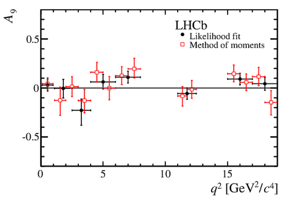
The $ C P$ -asymmetric observables in bins of $q^2$, determined from a maximum likelihood fit to the data. |
A3Pad.pdf [13 KiB] HiDef png [46 KiB] Thumbnail [25 KiB] *.C file |

|
|
A4Pad.pdf [13 KiB] HiDef png [46 KiB] Thumbnail [25 KiB] *.C file |
|
|
|
A5Pad.pdf [13 KiB] HiDef png [46 KiB] Thumbnail [25 KiB] *.C file |

|
|
|
A6Pad.pdf [13 KiB] HiDef png [47 KiB] Thumbnail [26 KiB] *.C file |
|
|
|
A7Pad.pdf [13 KiB] HiDef png [46 KiB] Thumbnail [26 KiB] *.C file |
|
|
|
A8Pad.pdf [13 KiB] HiDef png [47 KiB] Thumbnail [26 KiB] *.C file |

|
|
|
A9Pad.pdf [13 KiB] HiDef png [46 KiB] Thumbnail [25 KiB] *.C file |

|
|
|
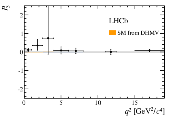
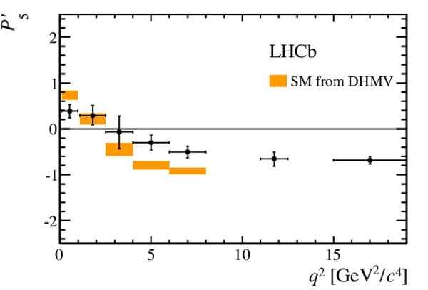
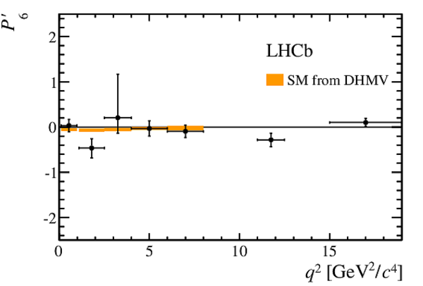
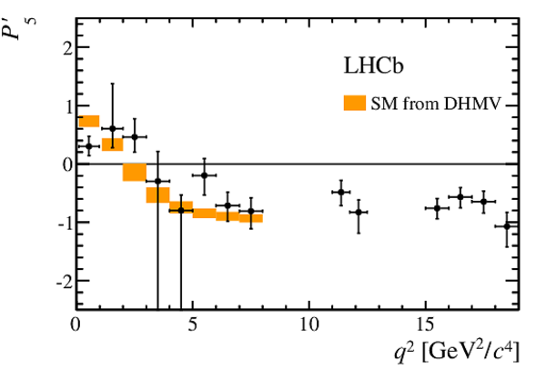
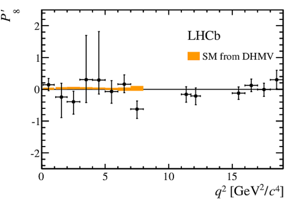
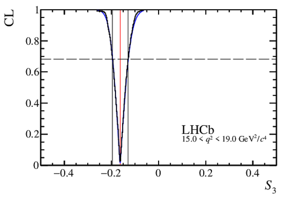
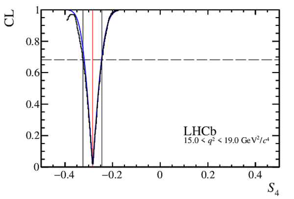
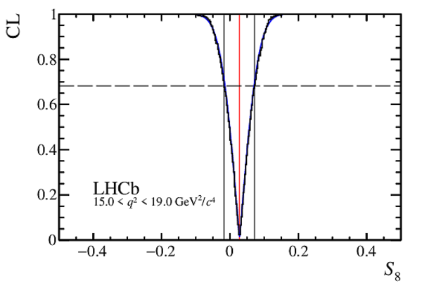
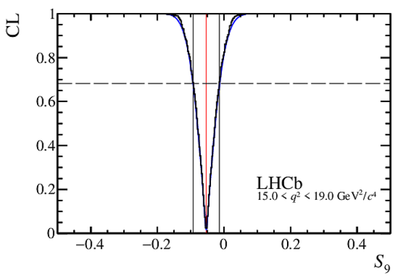
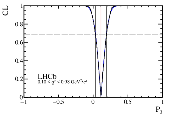
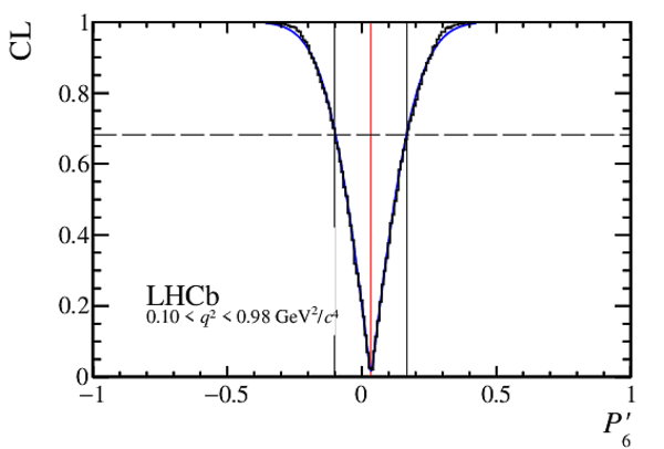
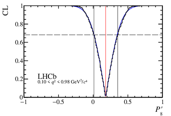
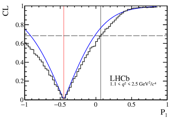
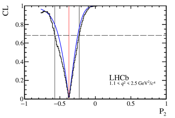
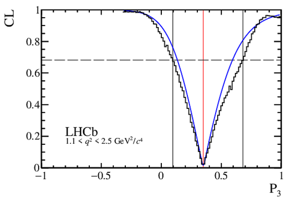
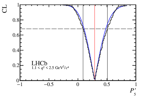
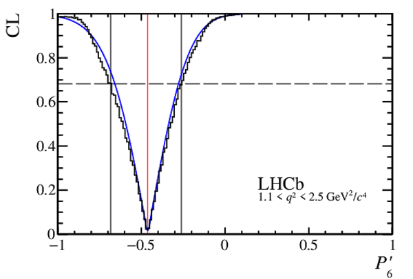
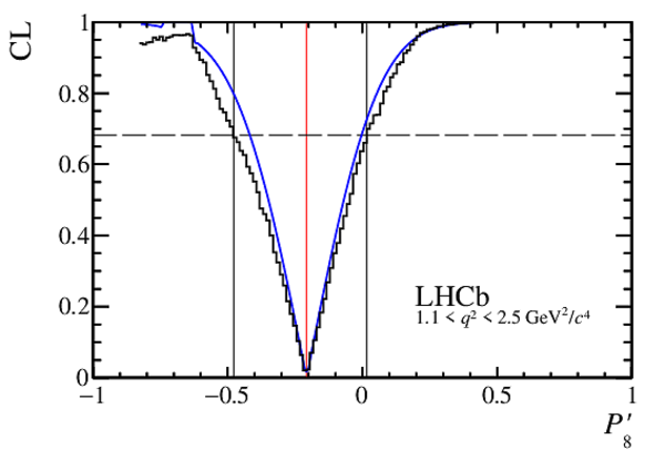
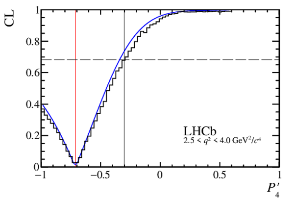
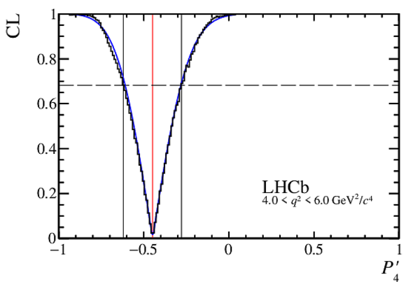
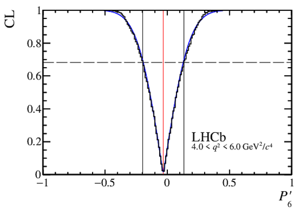
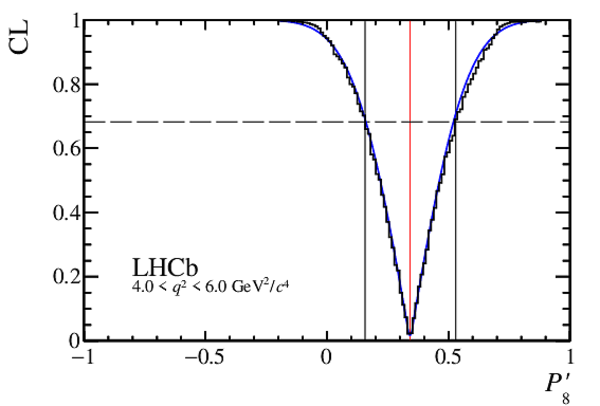
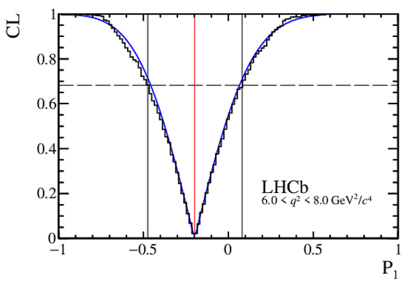
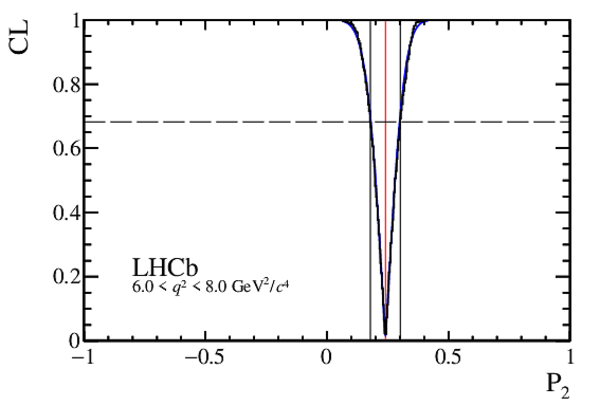
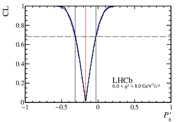
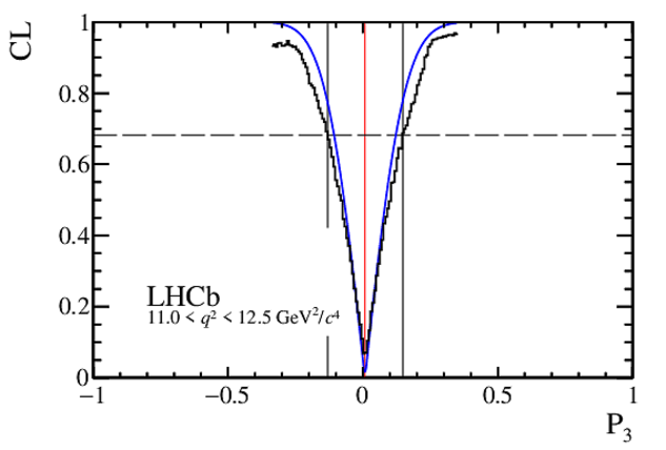
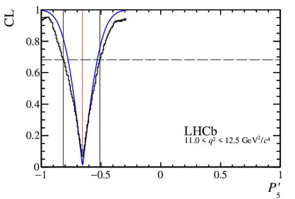
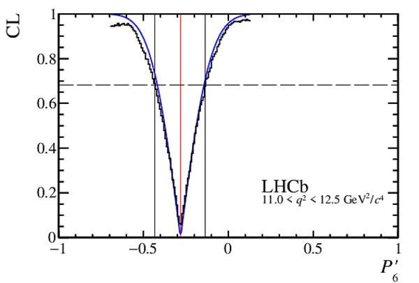
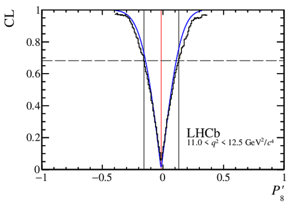
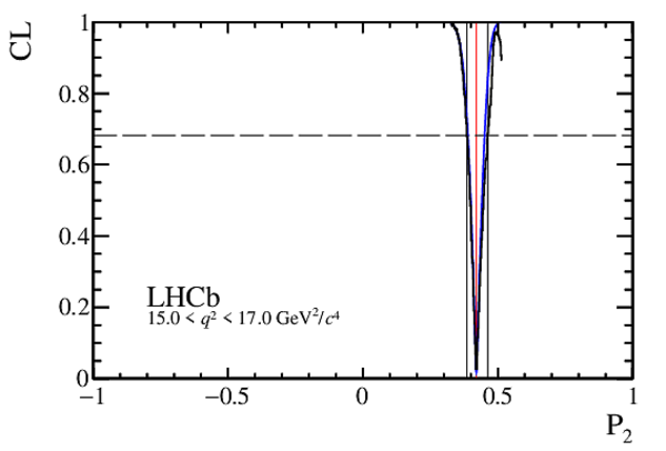
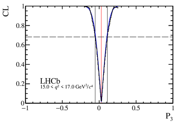
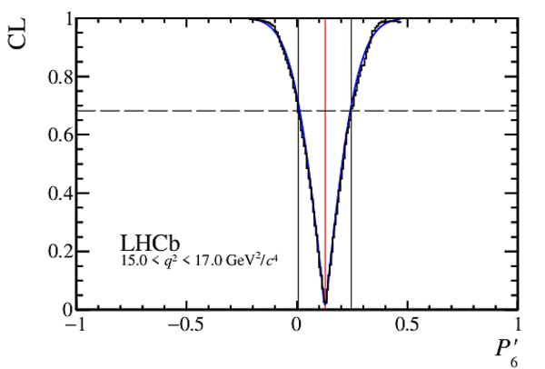
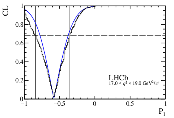
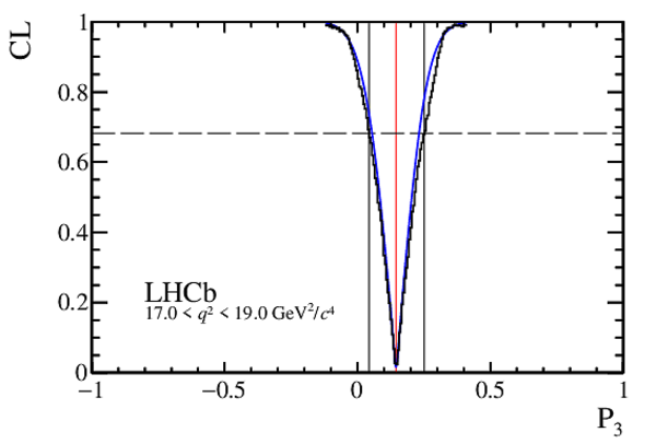
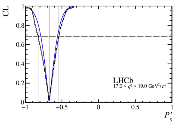
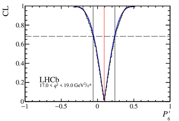
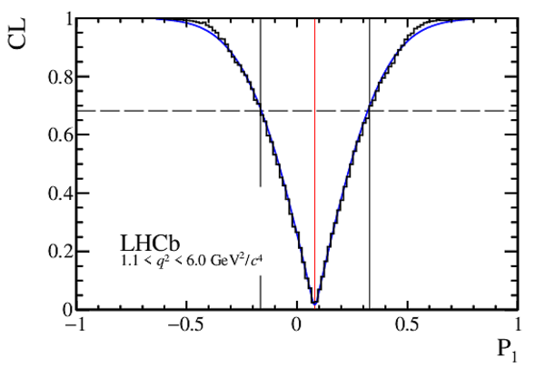
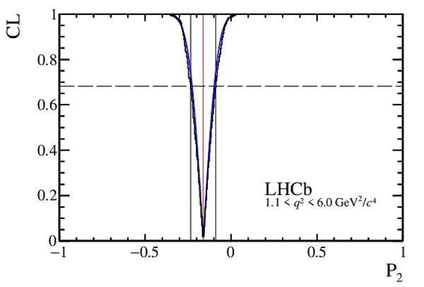
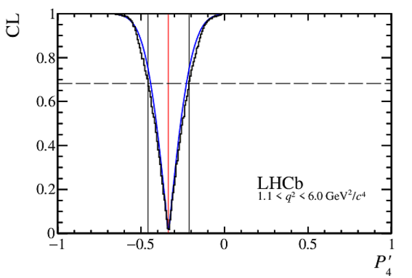
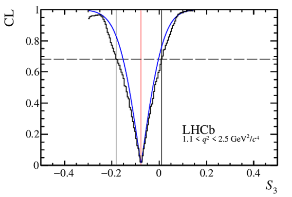
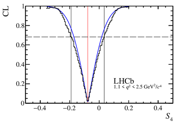
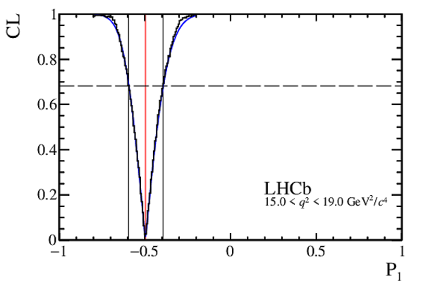
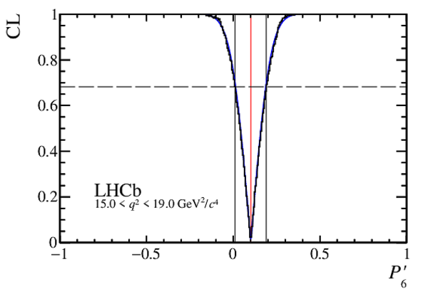
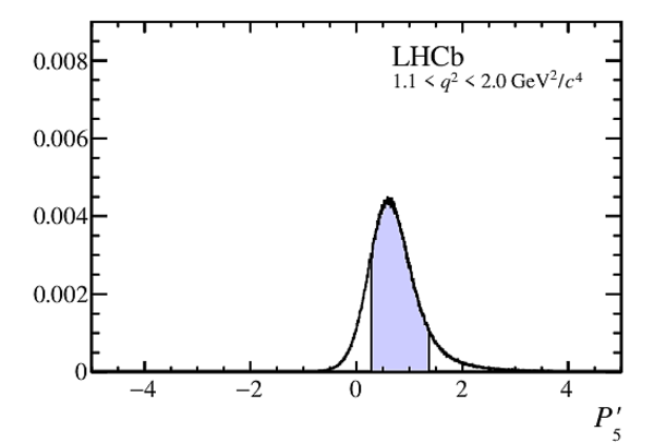
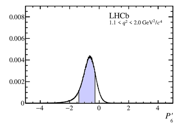
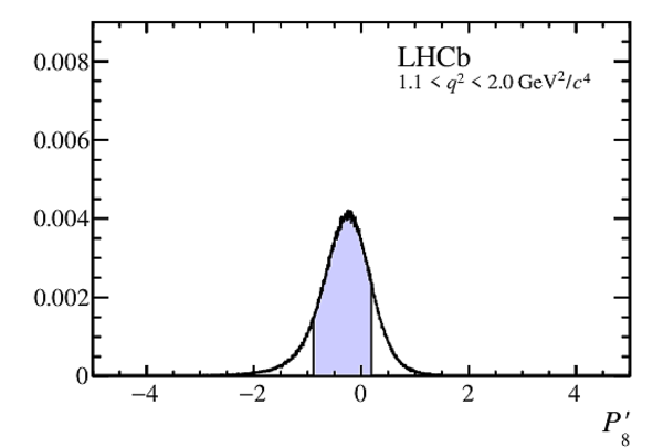
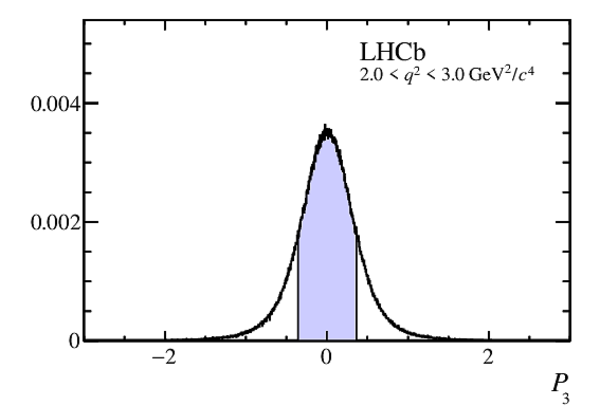
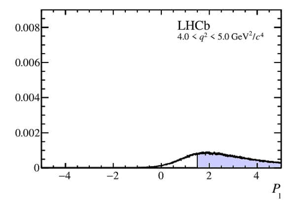
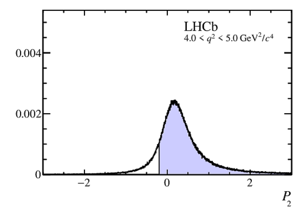
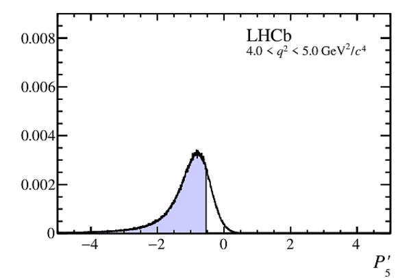
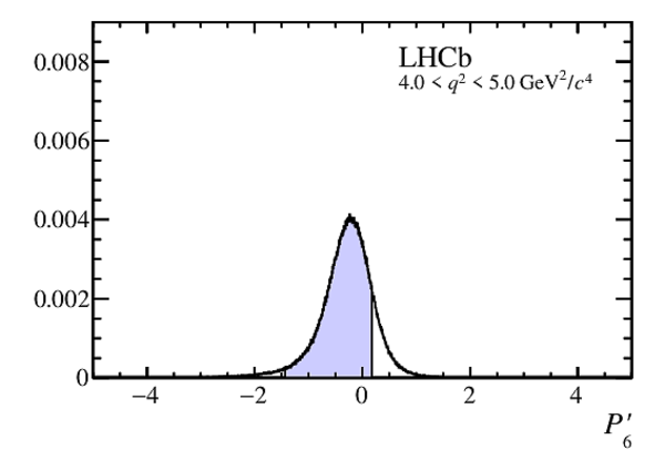
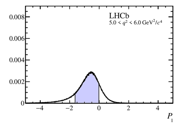
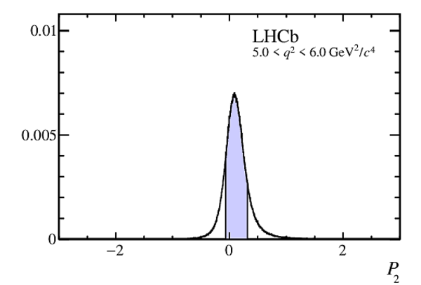
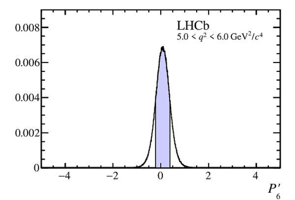
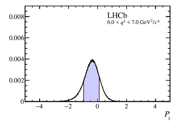
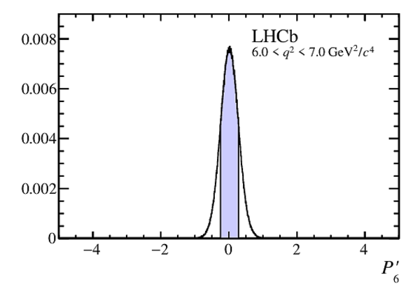
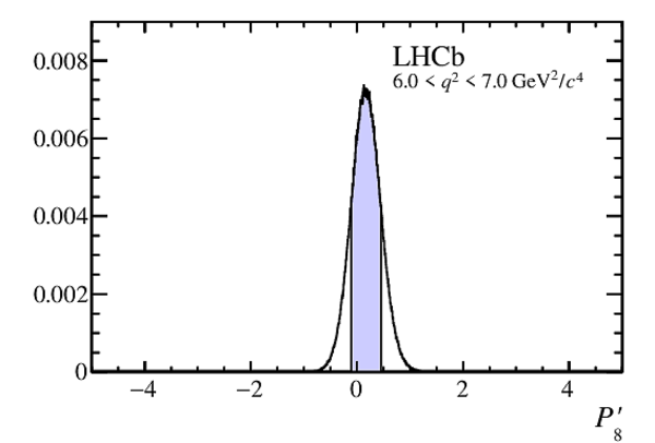
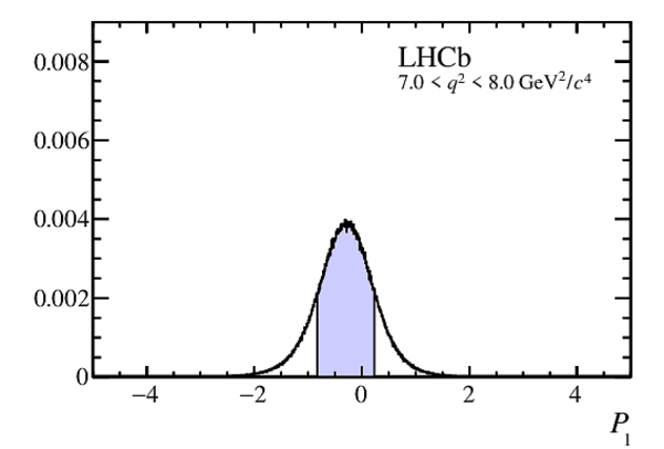
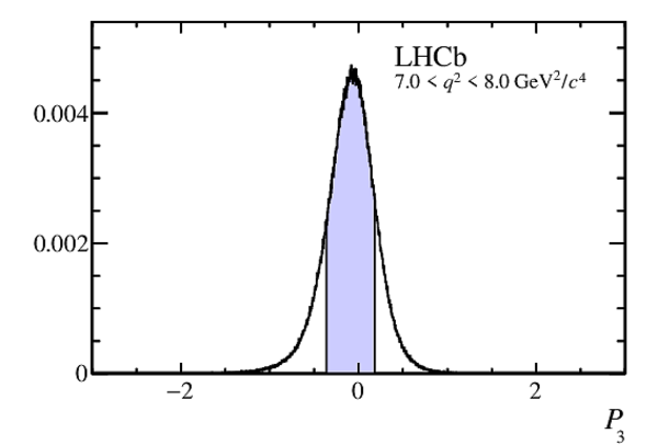
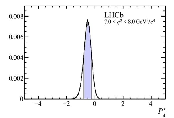
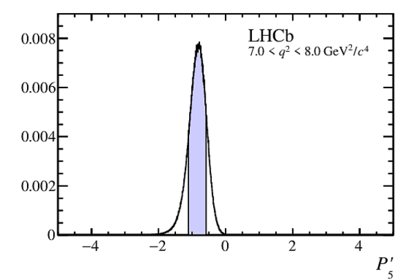
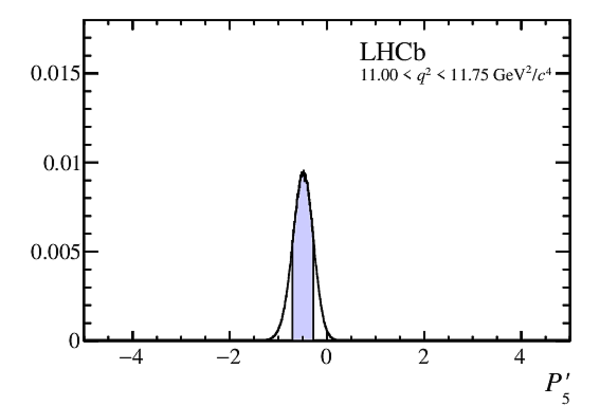
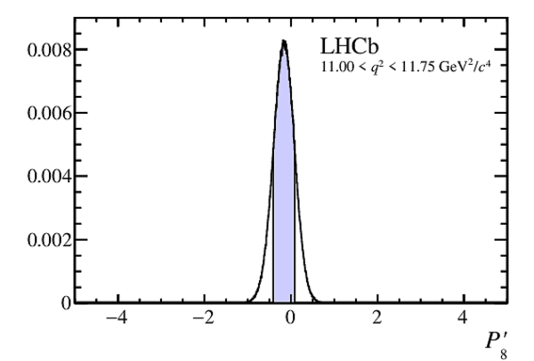
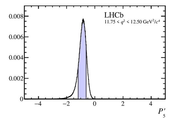
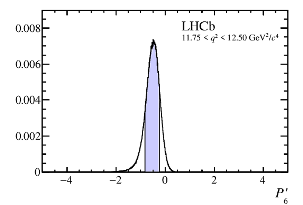
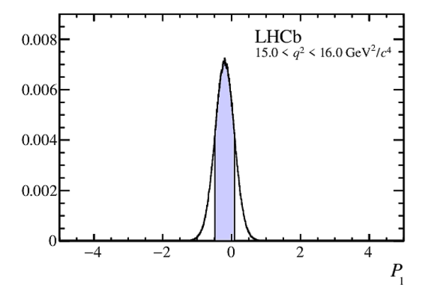
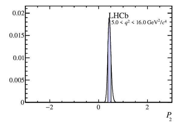
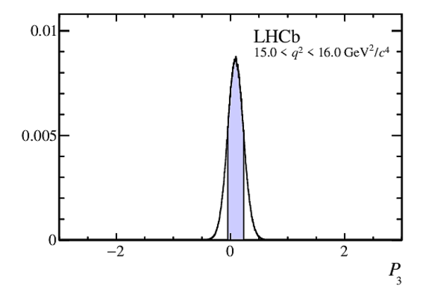
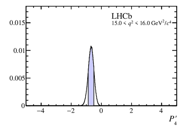
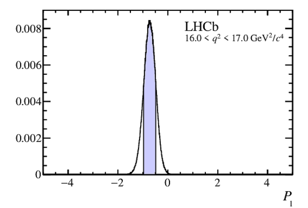
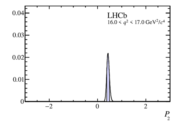
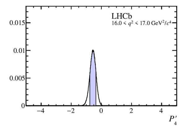
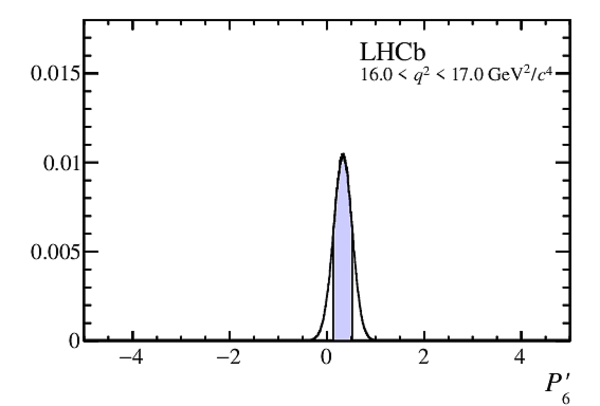
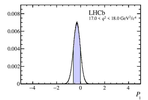
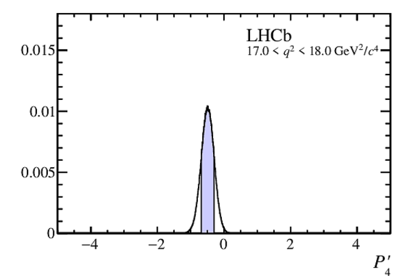
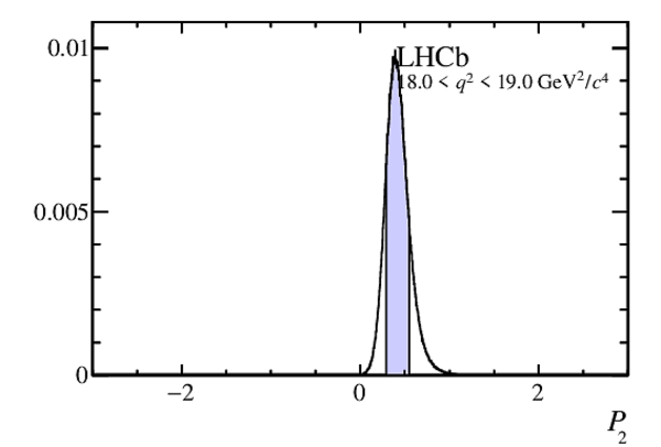
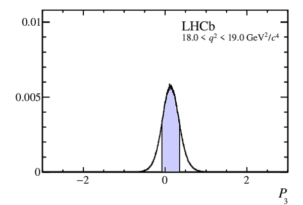
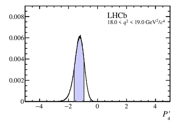
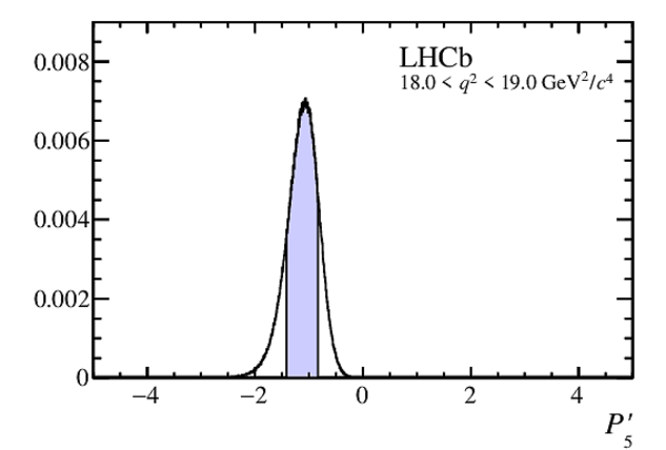
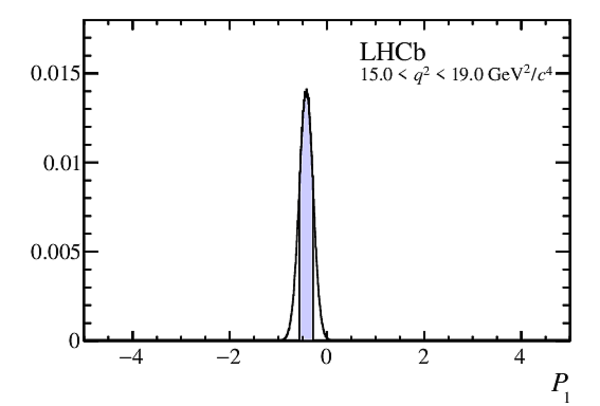
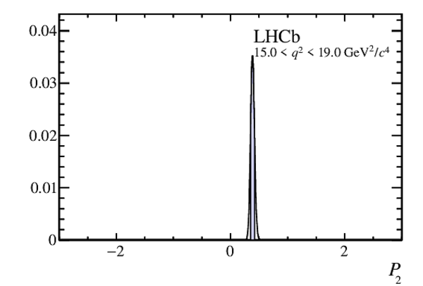
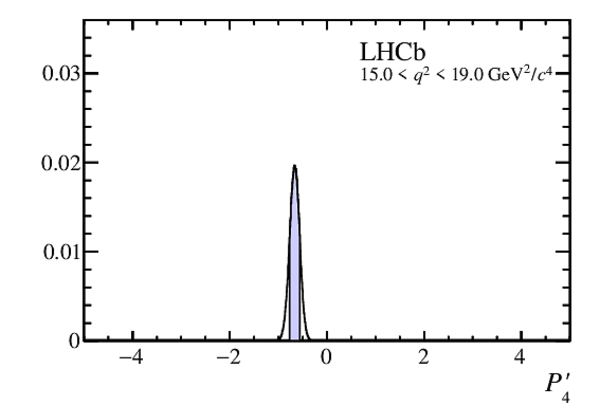
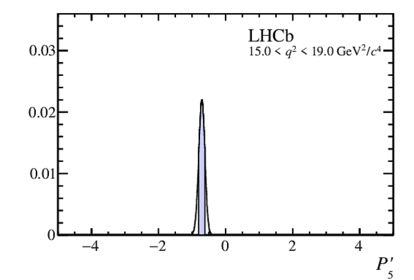
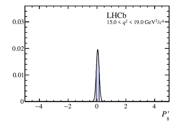
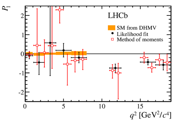
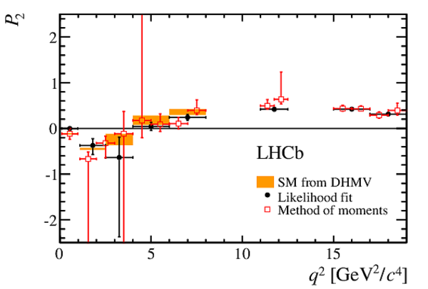
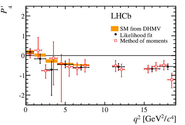
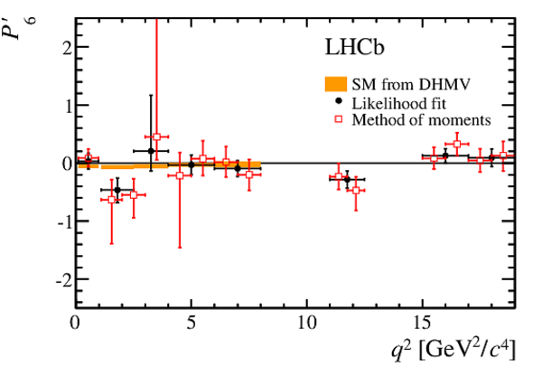
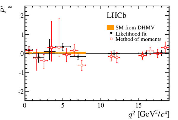
The optimised angular observables in bins of $q^2$, determined from a maximum likelihood fit to the data. The shaded boxes show the SM prediction taken from Ref. [14]. |
PBasis[..].pdf [14 KiB] HiDef png [77 KiB] Thumbnail [77 KiB] *.C file |

|
|
PBasis[..].pdf [14 KiB] HiDef png [74 KiB] Thumbnail [75 KiB] *.C file |

|
|
|
PBasis[..].pdf [14 KiB] HiDef png [74 KiB] Thumbnail [75 KiB] *.C file |
|
|
|
PBasis[..].pdf [14 KiB] HiDef png [77 KiB] Thumbnail [76 KiB] *.C file |

|
|
|
PBasis[..].pdf [14 KiB] HiDef png [75 KiB] Thumbnail [77 KiB] *.C file |
|
|
|
PBasis[..].pdf [14 KiB] HiDef png [75 KiB] Thumbnail [76 KiB] *.C file |
|
|
|
PBasis[..].pdf [14 KiB] HiDef png [75 KiB] Thumbnail [76 KiB] *.C file |

|
|
|
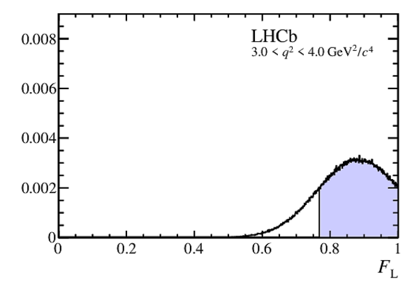
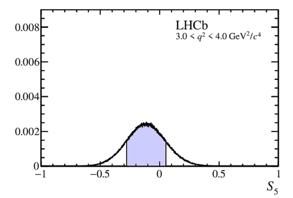
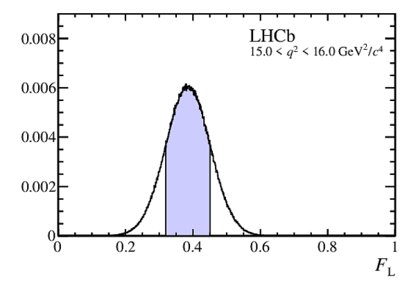
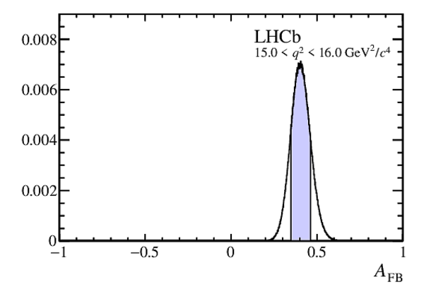
The $ C P$ -averaged observables in bins of $q^2$, determined from a moment analysis of the data. The shaded boxes show the SM predictions based on the prescription of Ref. [19]. |
moment[..].pdf [14 KiB] HiDef png [88 KiB] Thumbnail [82 KiB] *.C file |

|
|
moment[..].pdf [14 KiB] HiDef png [91 KiB] Thumbnail [86 KiB] *.C file |
|
|
|
moment[..].pdf [14 KiB] HiDef png [85 KiB] Thumbnail [83 KiB] *.C file |

|
|
|
moment[..].pdf [14 KiB] HiDef png [87 KiB] Thumbnail [84 KiB] *.C file |

|
|
|
moment[..].pdf [14 KiB] HiDef png [89 KiB] Thumbnail [85 KiB] *.C file |
|
|
|
moment[..].pdf [14 KiB] HiDef png [54 KiB] Thumbnail [31 KiB] *.C file |
|
|
|
moment[..].pdf [14 KiB] HiDef png [55 KiB] Thumbnail [32 KiB] *.C file |

|
|
|
moment[..].pdf [14 KiB] HiDef png [54 KiB] Thumbnail [31 KiB] *.C file |

|
|
|
The $ C P$ -asymmetric observables in bins of $q^2$, determined from a moment analysis of the data. |
moment[..].pdf [14 KiB] HiDef png [54 KiB] Thumbnail [31 KiB] *.C file |

|
|
moment[..].pdf [14 KiB] HiDef png [55 KiB] Thumbnail [31 KiB] *.C file |
|
|
|
moment[..].pdf [14 KiB] HiDef png [55 KiB] Thumbnail [31 KiB] *.C file |
|
|
|
moment[..].pdf [14 KiB] HiDef png [55 KiB] Thumbnail [31 KiB] *.C file |
|
|
|
moment[..].pdf [14 KiB] HiDef png [54 KiB] Thumbnail [31 KiB] *.C file |
|
|
|
moment[..].pdf [14 KiB] HiDef png [55 KiB] Thumbnail [31 KiB] *.C file |
|
|
|
moment[..].pdf [14 KiB] HiDef png [54 KiB] Thumbnail [31 KiB] *.C file |

|
|
|
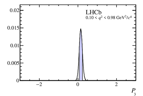
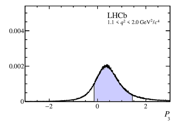
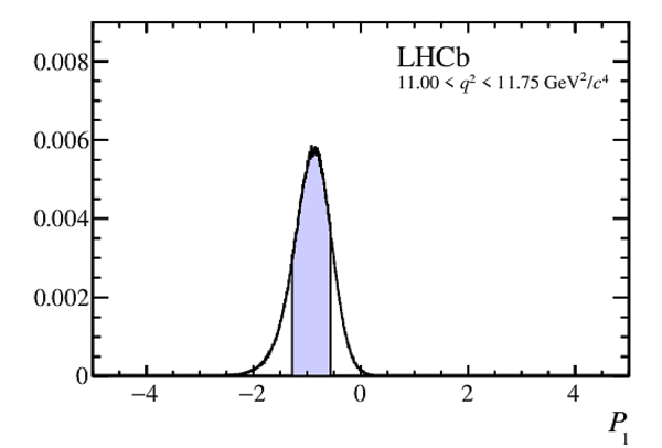
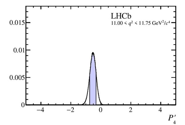
The optimised angular observables in bins of $q^2$, determined from a moment analysis of the data. The shaded boxes show the SM predictions taken from Ref. [14]. |
PBasis[..].pdf [15 KiB] HiDef png [88 KiB] Thumbnail [90 KiB] *.C file |

|
|
PBasis[..].pdf [14 KiB] HiDef png [87 KiB] Thumbnail [86 KiB] *.C file |

|
|
|
PBasis[..].pdf [15 KiB] HiDef png [84 KiB] Thumbnail [87 KiB] *.C file |

|
|
|
PBasis[..].pdf [15 KiB] HiDef png [88 KiB] Thumbnail [90 KiB] *.C file |

|
|
|
PBasis[..].pdf [15 KiB] HiDef png [87 KiB] Thumbnail [91 KiB] *.C file |
|
|
|
PBasis[..].pdf [15 KiB] HiDef png [84 KiB] Thumbnail [87 KiB] *.C file |

|
|
|
PBasis[..].pdf [15 KiB] HiDef png [87 KiB] Thumbnail [91 KiB] *.C file |
|
|
|
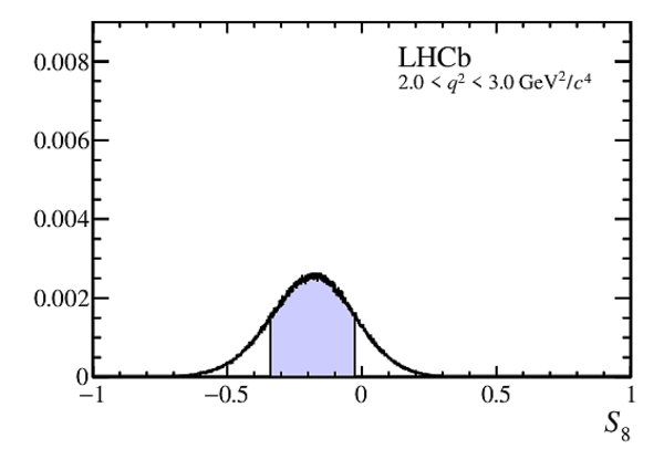
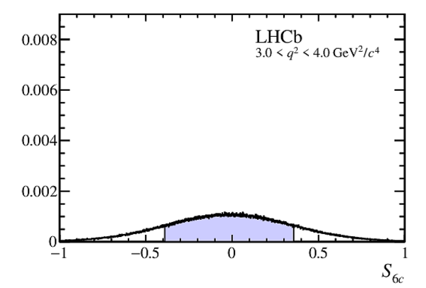
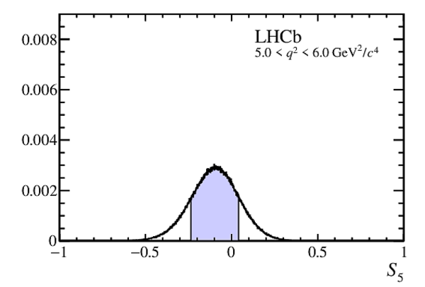
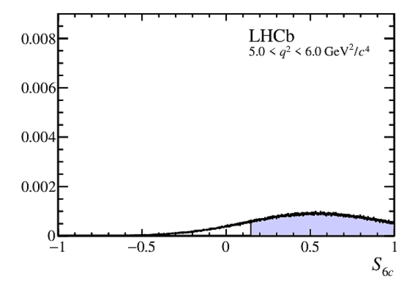
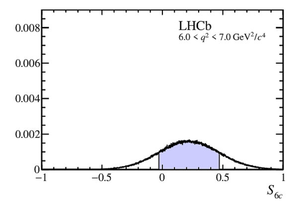
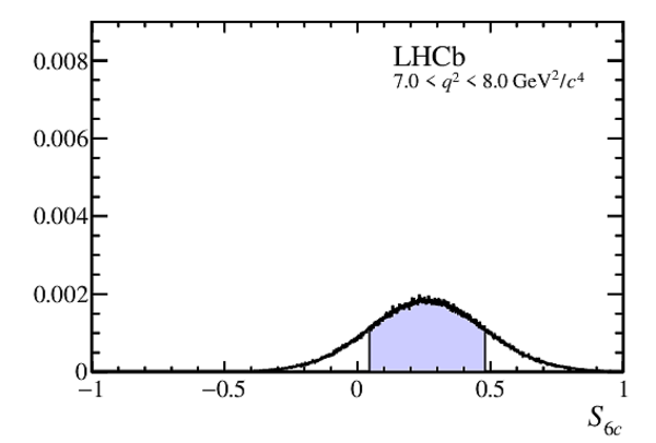
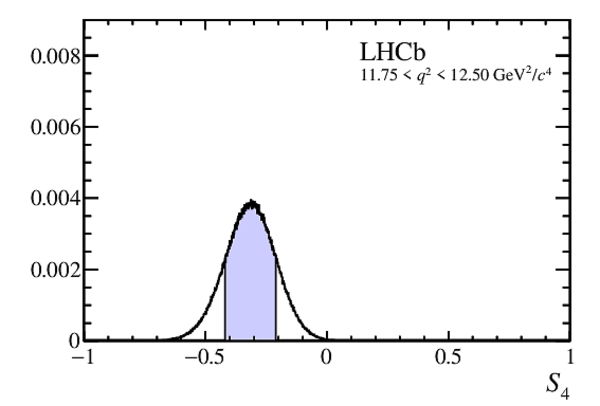
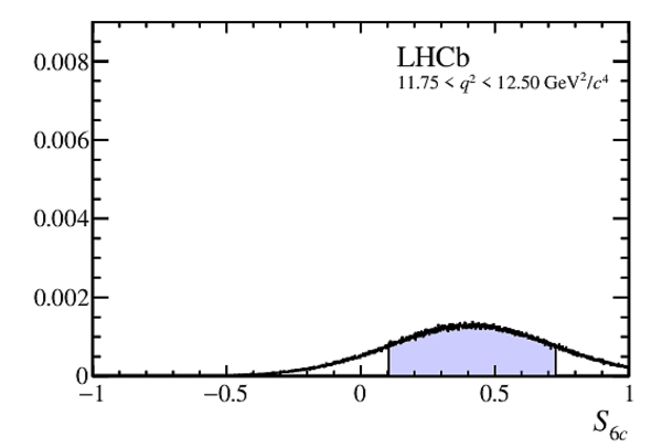
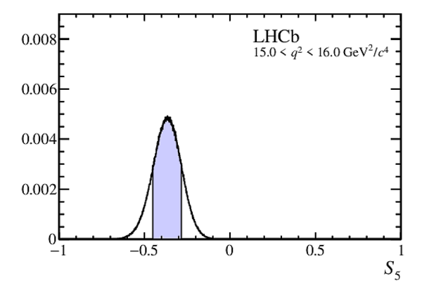
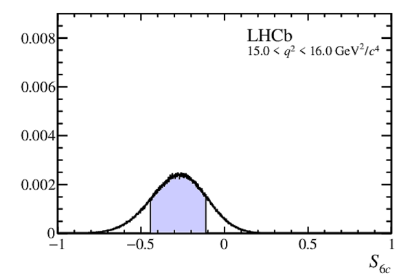
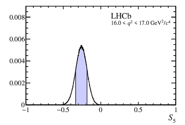
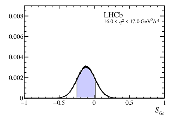
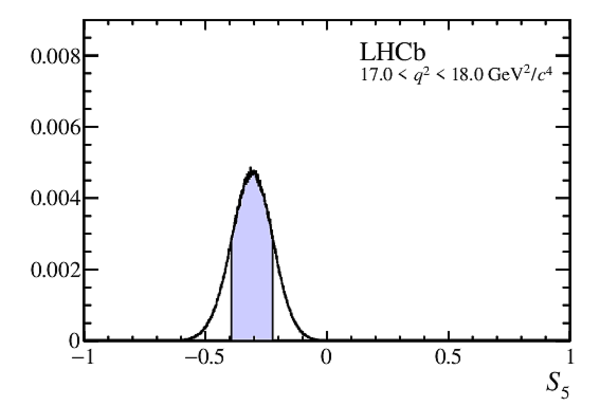
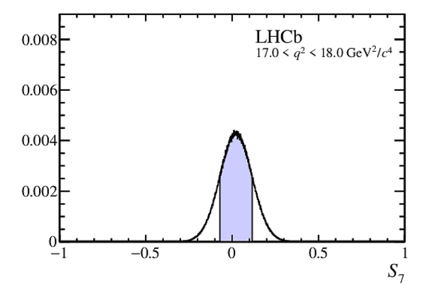
The observable $S_{6c}$ in bins of $q^2$, as determined from a moment analysis of the data. |
S6cPad.pdf [14 KiB] HiDef png [57 KiB] Thumbnail [36 KiB] *.C file |

|
|
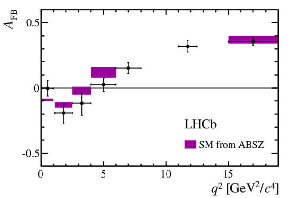
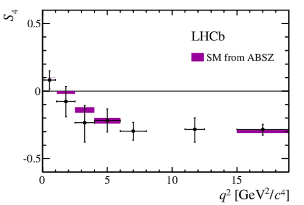
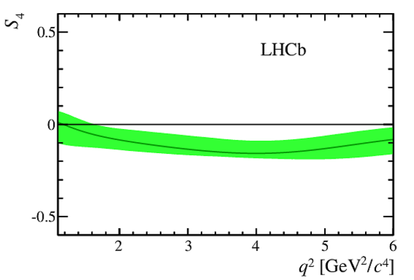
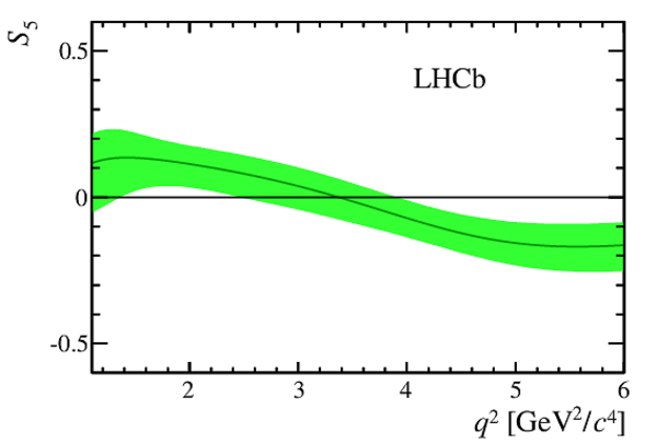
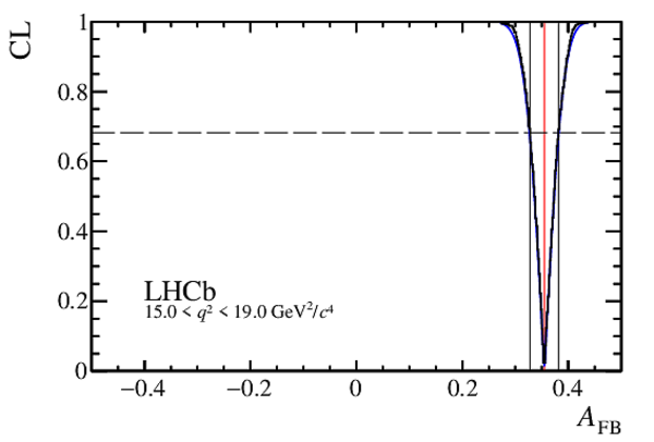
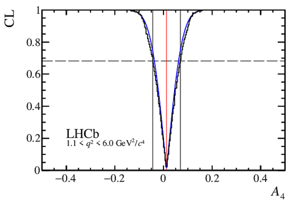
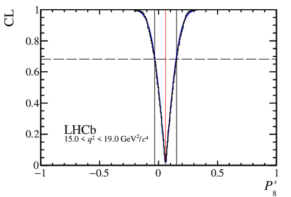
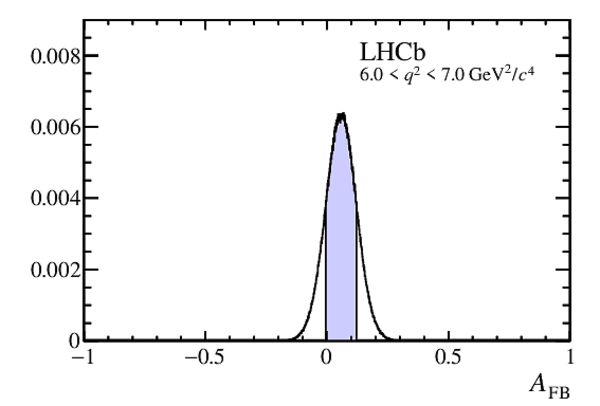
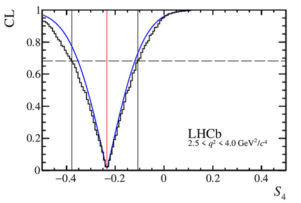
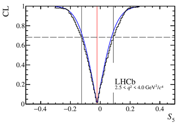
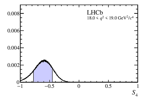
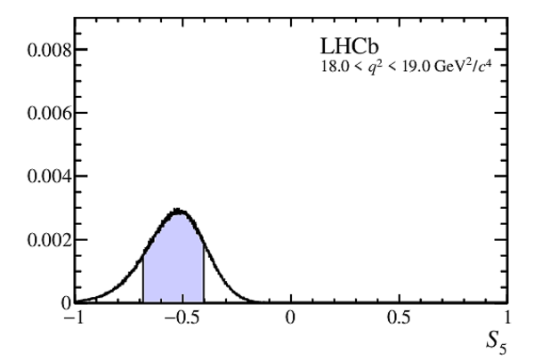
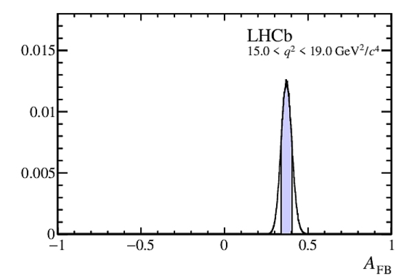
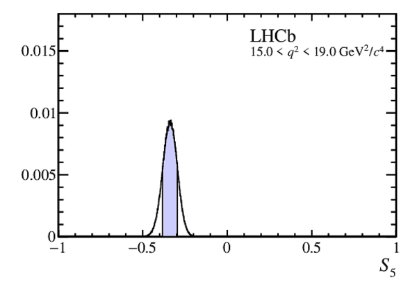
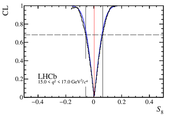
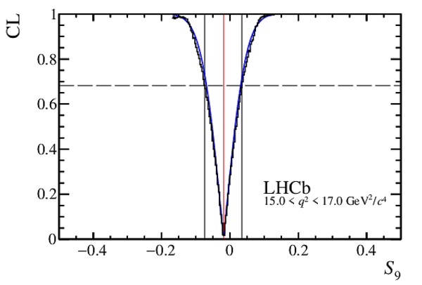
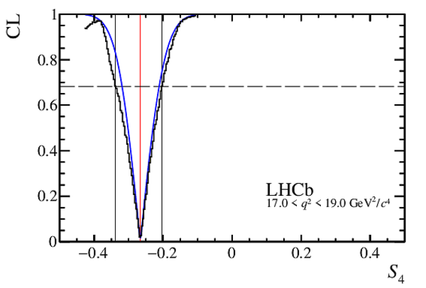
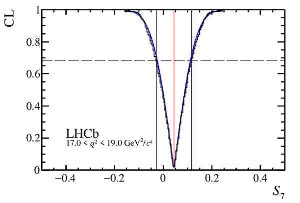
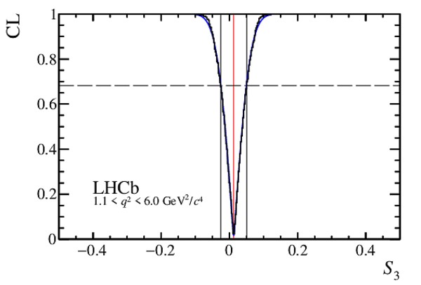
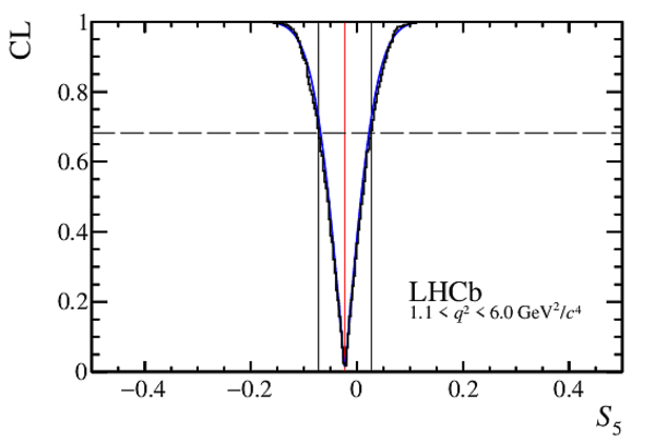
The observables $S_4$, $S_5$ and $A_{\rm FB}$ determined by fitting for the $ q^2$ dependent decay amplitudes. The line indicates the best-fit to the dataset. The band indicates the 68% interval on the bootstraps at each point in $ q^2$ . Note that, the correlation between points in the bands means it is not possible to extract the uncertainty on the zero-crossing points from these figures. |
amplit[..].pdf [25 KiB] HiDef png [107 KiB] Thumbnail [77 KiB] *.C file |
|
|
amplit[..].pdf [25 KiB] HiDef png [112 KiB] Thumbnail [80 KiB] *.C file |
|
|
|
amplit[..].pdf [25 KiB] HiDef png [111 KiB] Thumbnail [79 KiB] *.C file |

|
|
|
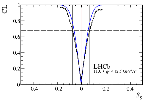
The $\Delta\chi^2$ distribution for the real part of the generalised vector-coupling strength, ${\cal C}_9$. This is determined from a fit to the results of the maximum likelihood fit of the $ C P$ -averaged observables. The SM central value is ${\rm Re}({\cal C}_9^{\rm SM}) = 4.27$ [11]. The best fit point is found to be at $\Delta{\rm Re}({\cal C}_9)= -1.04 \pm 0.25$. |
wilsonchi2.pdf [13 KiB] HiDef png [118 KiB] Thumbnail [91 KiB] *.C file |

|
|
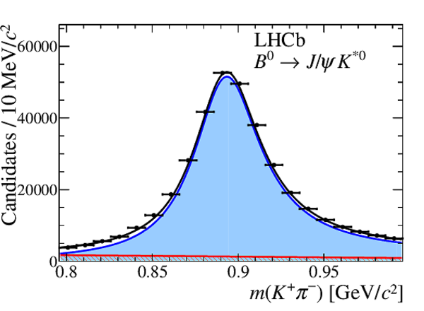
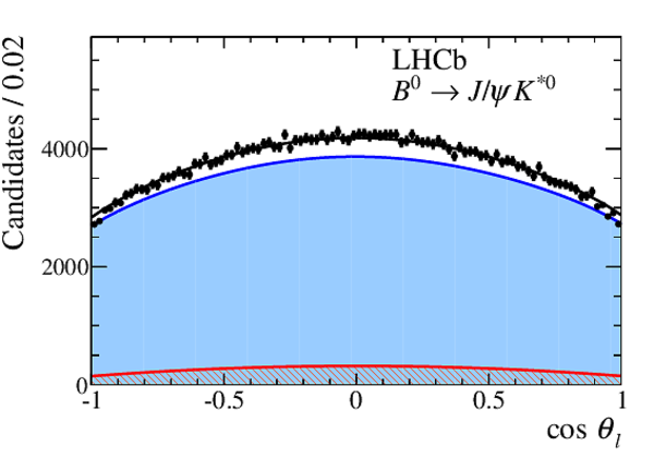
Angular and mass distribution of $ B ^0 \rightarrow { J \mskip -3mu/\mskip -2mu\psi \mskip 2mu} K ^{*0} $ candidates in data. A small signal component is also included in the fit to account for $\overline{ B }{} {}^0_ s \rightarrow { J \mskip -3mu/\mskip -2mu\psi \mskip 2mu} K ^{*0} $ decays. Overlaid are the projections of the total fitted distribution (black line) and its different components. The signal is shown by the solid blue component and the background by the red hatched component. |
mlogjpsi.pdf [73 KiB] HiDef png [576 KiB] Thumbnail [400 KiB] *.C file |
|
|
mkpijpsi.pdf [19 KiB] HiDef png [232 KiB] Thumbnail [183 KiB] *.C file |
|
|
|
costhe[..].pdf [42 KiB] HiDef png [236 KiB] Thumbnail [173 KiB] *.C file |
|
|
|
costhe[..].pdf [38 KiB] HiDef png [209 KiB] Thumbnail [163 KiB] *.C file |

|
|
|
phijpsi.pdf [41 KiB] HiDef png [222 KiB] Thumbnail [169 KiB] *.C file |

|
|
|
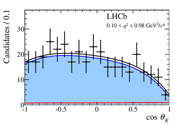
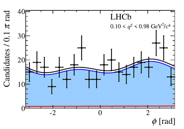
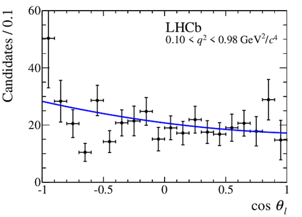
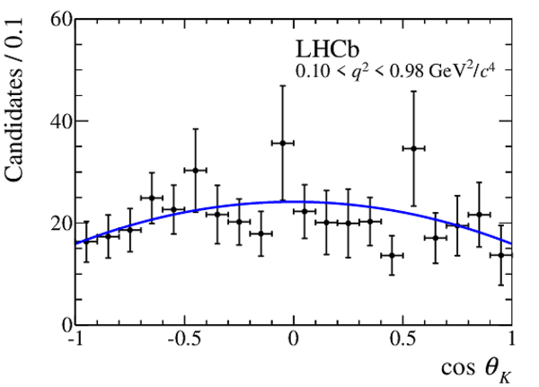
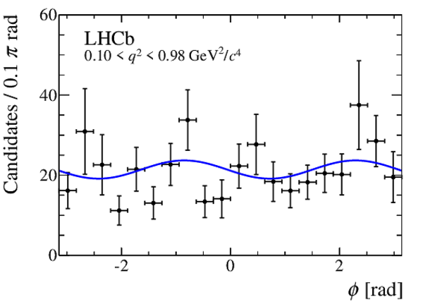
Angular and mass distributions for $0.10<q^2<0.98 {\mathrm{ Ge V^2 /}c^4} $. The distributions of $m( K ^+ \pi ^- )$ and the three decay angles are given for candidates in the signal mass window $\pm50 {\mathrm{ Me V /}c^2} $ around the known $ B ^0 $ mass. Overlaid are the projections of the total fitted distribution (black line) and its different components. The signal is shown by the solid blue component and the background by the red hatched component. |
m0.pdf [71 KiB] HiDef png [186 KiB] Thumbnail [147 KiB] *.C file |
|
|
mkpi0sig.pdf [20 KiB] HiDef png [212 KiB] Thumbnail [168 KiB] *.C file |

|
|
|
costhe[..].pdf [20 KiB] HiDef png [215 KiB] Thumbnail [167 KiB] *.C file |

|
|
|
costhe[..].pdf [19 KiB] HiDef png [205 KiB] Thumbnail [167 KiB] *.C file |
|
|
|
phi0sig.pdf [19 KiB] HiDef png [202 KiB] Thumbnail [167 KiB] *.C file |
|
|
|
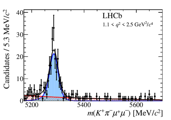
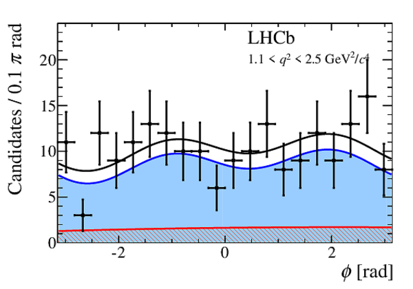
Angular and mass distributions for $1.1<q^2<2.5 {\mathrm{ Ge V^2 /}c^4} $. The distributions of $m( K ^+ \pi ^- )$ and the three decay angles are given for candidates in the signal mass window $\pm50 {\mathrm{ Me V /}c^2} $ around the known $ B ^0 $ mass. Overlaid are the projections of the total fitted distribution (black line) and its different components. The signal is shown by the solid blue component and the background by the red hatched component. |
m1.pdf [73 KiB] HiDef png [227 KiB] Thumbnail [180 KiB] *.C file |
|
|
mkpi1sig.pdf [20 KiB] HiDef png [269 KiB] Thumbnail [208 KiB] *.C file |

|
|
|
costhe[..].pdf [20 KiB] HiDef png [254 KiB] Thumbnail [191 KiB] *.C file |

|
|
|
costhe[..].pdf [20 KiB] HiDef png [230 KiB] Thumbnail [181 KiB] *.C file |
|
|
|
phi1sig.pdf [19 KiB] HiDef png [260 KiB] Thumbnail [201 KiB] *.C file |
|
|
|
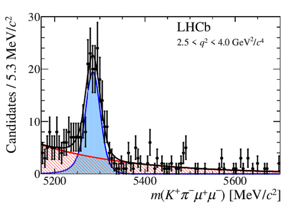
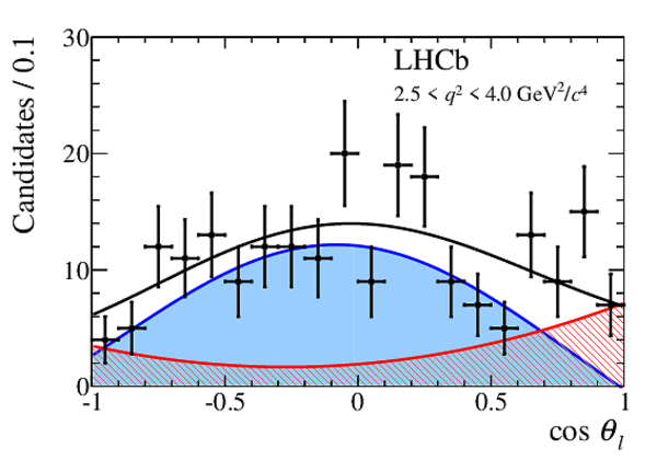
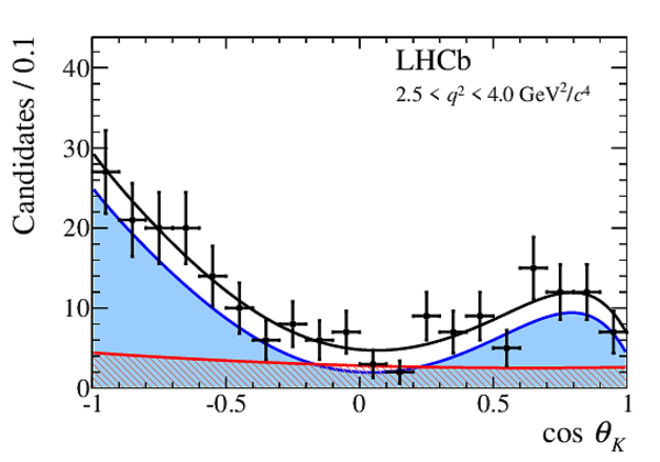
Angular and mass distributions for $2.5<q^2<4.0 {\mathrm{ Ge V^2 /}c^4} $. The distributions of $m( K ^+ \pi ^- )$ and the three decay angles are given for candidates in the signal mass window $\pm50 {\mathrm{ Me V /}c^2} $ around the known $ B ^0 $ mass. Overlaid are the projections of the total fitted distribution (black line) and its different components. The signal is shown by the solid blue component and the background by the red hatched component. |
m2.pdf [74 KiB] HiDef png [281 KiB] Thumbnail [215 KiB] *.C file |
|
|
mkpi2sig.pdf [20 KiB] HiDef png [293 KiB] Thumbnail [228 KiB] *.C file |

|
|
|
costhe[..].pdf [20 KiB] HiDef png [308 KiB] Thumbnail [226 KiB] *.C file |
|
|
|
costhe[..].pdf [20 KiB] HiDef png [268 KiB] Thumbnail [202 KiB] *.C file |
|
|
|
phi2sig.pdf [19 KiB] HiDef png [306 KiB] Thumbnail [226 KiB] *.C file |

|
|
|
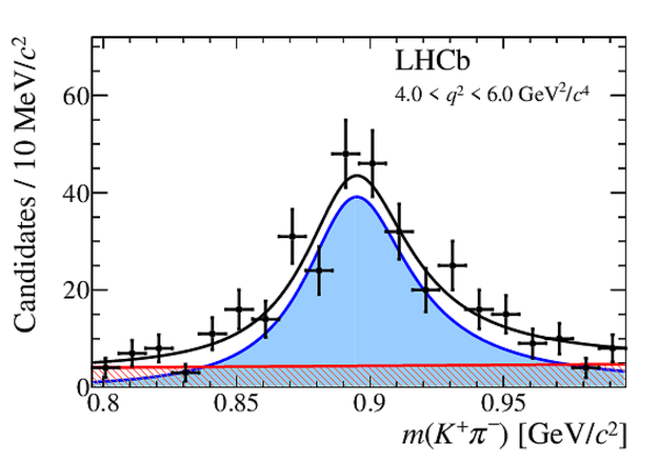
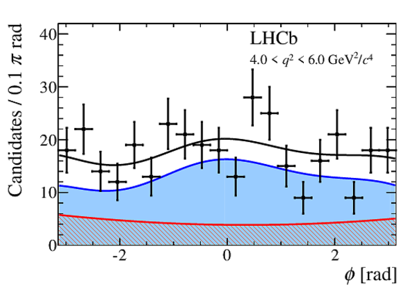
Angular and mass distributions for $4.0<q^2<6.0 {\mathrm{ Ge V^2 /}c^4} $. The distributions of $m( K ^+ \pi ^- )$ and the three decay angles are given for candidates in the signal mass window $\pm50 {\mathrm{ Me V /}c^2} $ around the known $ B ^0 $ mass. Overlaid are the projections of the total fitted distribution (black line) and its different components. The signal is shown by the solid blue component and the background by the red hatched component. |
m3.pdf [74 KiB] HiDef png [264 KiB] Thumbnail [201 KiB] *.C file |

|
|
mkpi3sig.pdf [20 KiB] HiDef png [261 KiB] Thumbnail [210 KiB] *.C file |
|
|
|
costhe[..].pdf [20 KiB] HiDef png [334 KiB] Thumbnail [235 KiB] *.C file |

|
|
|
costhe[..].pdf [20 KiB] HiDef png [278 KiB] Thumbnail [206 KiB] *.C file |

|
|
|
phi3sig.pdf [20 KiB] HiDef png [314 KiB] Thumbnail [232 KiB] *.C file |
|
|
|
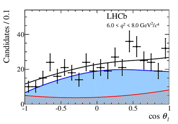
Angular and mass distributions for $6.0<q^2<8.0 {\mathrm{ Ge V^2 /}c^4} $. The distributions of $m( K ^+ \pi ^- )$ and the three decay angles are given for candidates in the signal mass window $\pm50 {\mathrm{ Me V /}c^2} $ around the known $ B ^0 $ mass. Overlaid are the projections of the total fitted distribution (black line) and its different components. The signal is shown by the blue shaded area and the background by the red hatched area. |
m4.pdf [75 KiB] HiDef png [261 KiB] Thumbnail [199 KiB] *.C file |

|
|
mkpi4sig.pdf [20 KiB] HiDef png [256 KiB] Thumbnail [211 KiB] *.C file |

|
|
|
costhe[..].pdf [19 KiB] HiDef png [287 KiB] Thumbnail [210 KiB] *.C file |
|
|
|
costhe[..].pdf [20 KiB] HiDef png [283 KiB] Thumbnail [206 KiB] *.C file |

|
|
|
phi4sig.pdf [19 KiB] HiDef png [324 KiB] Thumbnail [237 KiB] *.C file |

|
|
|
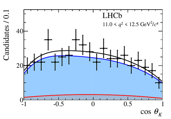
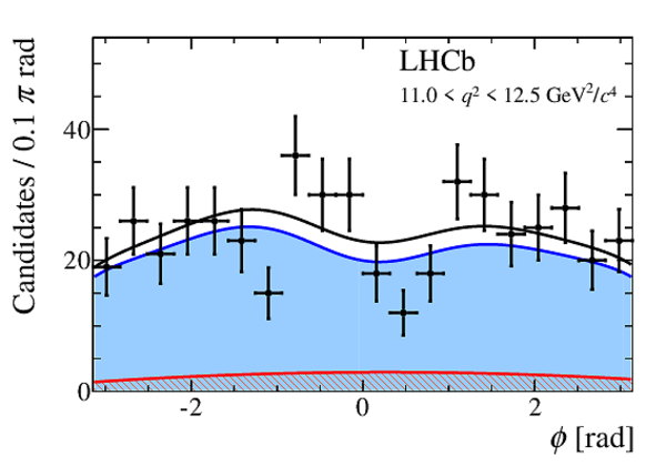
Angular and mass distributions for $11.0<q^2<12.5 {\mathrm{ Ge V^2 /}c^4} $. The distributions of $m( K ^+ \pi ^- )$ and the three decay angles are given for candidates in the signal mass window $\pm50 {\mathrm{ Me V /}c^2} $ around the known $ B ^0 $ mass. Overlaid are the projections of the total fitted distribution (black line) and its different components. The signal is shown by the blue shaded area and the background by the red hatched area. |
m5.pdf [74 KiB] HiDef png [220 KiB] Thumbnail [170 KiB] *.C file |
|
|
mkpi5sig.pdf [20 KiB] HiDef png [217 KiB] Thumbnail [172 KiB] *.C file |

|
|
|
costhe[..].pdf [20 KiB] HiDef png [225 KiB] Thumbnail [171 KiB] *.C file |

|
|
|
costhe[..].pdf [19 KiB] HiDef png [240 KiB] Thumbnail [182 KiB] *.C file |
|
|
|
phi5sig.pdf [19 KiB] HiDef png [235 KiB] Thumbnail [179 KiB] *.C file |
|
|
|
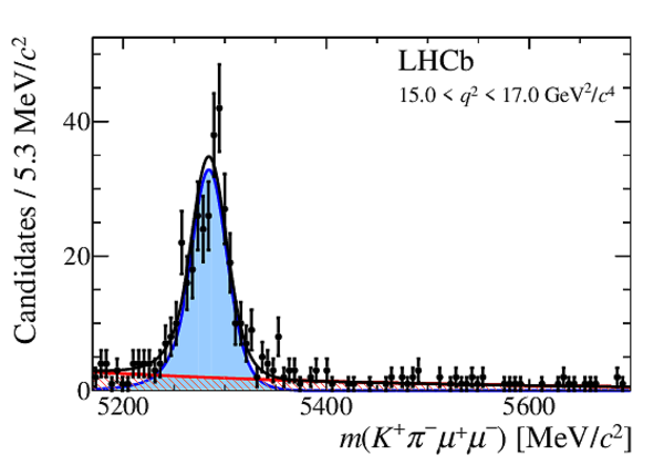
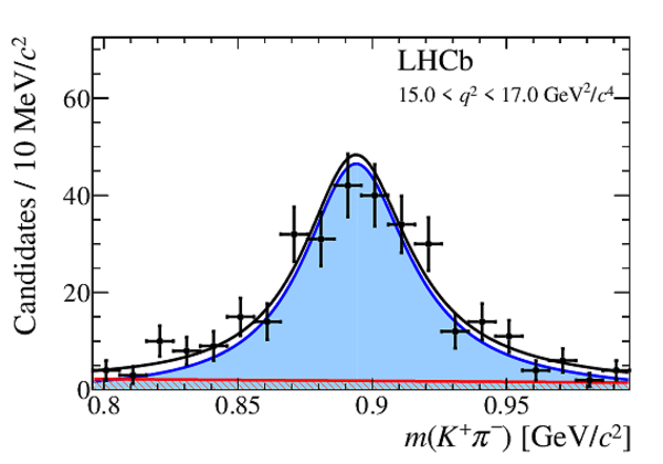
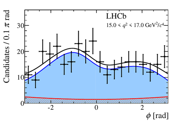
Angular and mass distributions for $15.0<q^2<17.0 {\mathrm{ Ge V^2 /}c^4} $. The distributions of $m( K ^+ \pi ^- )$ and the three decay angles are given for candidates in the signal mass window $\pm50 {\mathrm{ Me V /}c^2} $ around the known $ B ^0 $ mass. Overlaid are the projections of the total fitted distribution (black line) and its different components. The signal is shown by the blue shaded area and the background by the red hatched area. |
m6.pdf [73 KiB] HiDef png [224 KiB] Thumbnail [174 KiB] *.C file |
|
|
mkpi6sig.pdf [20 KiB] HiDef png [231 KiB] Thumbnail [185 KiB] *.C file |
|
|
|
costhe[..].pdf [19 KiB] HiDef png [221 KiB] Thumbnail [168 KiB] *.C file |

|
|
|
costhe[..].pdf [20 KiB] HiDef png [253 KiB] Thumbnail [194 KiB] *.C file |

|
|
|
phi6sig.pdf [20 KiB] HiDef png [255 KiB] Thumbnail [190 KiB] *.C file |
|
|
|
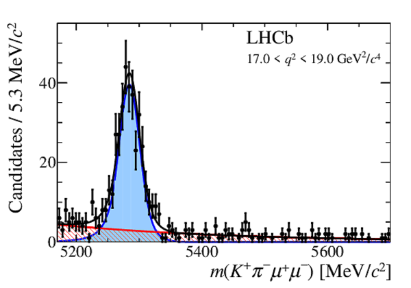
Angular and mass distributions for $17.0<q^2<19.0 {\mathrm{ Ge V^2 /}c^4} $. The distributions of $m( K ^+ \pi ^- )$ and the three decay angles are given for candidates in the signal mass window $\pm50 {\mathrm{ Me V /}c^2} $ around the known $ B ^0 $ mass. Overlaid are the projections of the total fitted distribution (black line) and its different components. The signal is shown by the blue shaded area and the background by the red hatched area. |
m7.pdf [74 KiB] HiDef png [238 KiB] Thumbnail [184 KiB] *.C file |
|
|
mkpi7sig.pdf [20 KiB] HiDef png [236 KiB] Thumbnail [189 KiB] *.C file |

|
|
|
costhe[..].pdf [20 KiB] HiDef png [245 KiB] Thumbnail [185 KiB] *.C file |

|
|
|
costhe[..].pdf [20 KiB] HiDef png [256 KiB] Thumbnail [199 KiB] *.C file |

|
|
|
phi7sig.pdf [19 KiB] HiDef png [257 KiB] Thumbnail [199 KiB] *.C file |

|
|
|
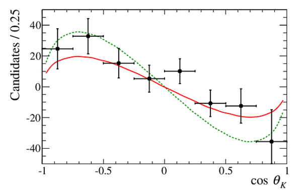
Angular and mass distributions for $15.0 <q^2< 19.0 {\mathrm{ Ge V^2 /}c^4} $. The distributions of $m( K ^+ \pi ^- )$ and the three decay angles are given for candidates in the signal mass window $\pm50 {\mathrm{ Me V /}c^2} $ around the known $ B ^0 $ mass. Overlaid are the projections of the total fitted distribution (black line) and its different components. The signal is shown by the blue shaded area and the background by the red hatched area. |
m9.pdf [75 KiB] HiDef png [217 KiB] Thumbnail [169 KiB] *.C file |

|
|
mkpi9sig.pdf [20 KiB] HiDef png [226 KiB] Thumbnail [179 KiB] *.C file |

|
|
|
costhe[..].pdf [20 KiB] HiDef png [218 KiB] Thumbnail [167 KiB] *.C file |

|
|
|
costhe[..].pdf [19 KiB] HiDef png [236 KiB] Thumbnail [180 KiB] *.C file |

|
|
|
phi9sig.pdf [20 KiB] HiDef png [232 KiB] Thumbnail [184 KiB] *.C file |

|
|
|
Animated gif made out of all figures. |
PAPER-2015-051.gif Thumbnail |

|
Tables and captions
|
Angular observables $I_j$ and their corresponding angular terms for dimuon masses that are much larger than twice the muon mass. The terms in the lower part of the table arise from the $ K ^+ \pi ^- $ S-wave contribution to the $ K ^+ \pi ^- \mu ^+\mu ^- $ final state. The $\bar{I}_i$ coefficients are obtained by making the substitution ${\cal A} \rightarrow \bar{{\cal A}}$, i.e. by complex conjugation of the weak phases in the amplitudes. |
Table_1.pdf [63 KiB] HiDef png [219 KiB] Thumbnail [110 KiB] tex code |

|
|
Summary of the different sources of systematic uncertainty on the angular observables. Upper limits or typical ranges are quoted for the different groups of observables. The column labelled $q^2_0$ corresponds to the zero-crossing points of $S_4$, $S_5$ and $A_{\rm FB}$. |
Table_2.pdf [44 KiB] HiDef png [89 KiB] Thumbnail [39 KiB] tex code |

|
|
$ C P$ -averaged angular observables evaluated by the unbinned maximum likelihood fit, in the range $1.1 < q^2 < 6.0 \mathrm{ Ge V} ^{2}/c^{4}$ and $15.0 < q^2 < 19.0 \mathrm{ Ge V} ^{2}/c^{4}$. The first uncertainties are statistical and the second systematic. |
Table_3.pdf [52 KiB] HiDef png [337 KiB] Thumbnail [164 KiB] tex code |

|
|
$ C P$ -averaged angular observables evaluated by the unbinned maximum likelihood fit. The first uncertainties are statistical and the second systematic. |
Table_4.pdf [52 KiB] HiDef png [295 KiB] Thumbnail [135 KiB] tex code |

|
|
$ C P$ -asymmetric angular observables evaluated by the unbinned maximum likelihood fit. The first uncertainties are statistical and the second systematic. |
Table_5.pdf [51 KiB] HiDef png [262 KiB] Thumbnail [120 KiB] tex code |

|
|
Optimised angular observables evaluated by the unbinned maximum likelihood fit. The first uncertainties are statistical and the second systematic. |
Table_6.pdf [51 KiB] HiDef png [262 KiB] Thumbnail [126 KiB] tex code |

|
|
$ C P$ -averaged angular observables evaluated using the method of moments. The first uncertainties are statistical and the second systematic. |
Table_7.pdf [54 KiB] HiDef png [406 KiB] Thumbnail [175 KiB] tex code |

|
|
$ C P$ -asymmetries evaluated using the method of moments. The first uncertainties are statistical and the second systematic. |
Table_8.pdf [52 KiB] HiDef png [328 KiB] Thumbnail [136 KiB] tex code |

|
|
Optimised observables evaluated using the method of moments. The first uncertainties are statistical and the second systematic. |
Table_9.pdf [52 KiB] HiDef png [328 KiB] Thumbnail [144 KiB] tex code |

|
|
Correlation matrix for the $ C P$ -averaged observables from the maximum likelihood fit in the bin $0.10<q^2<0.98 {\mathrm{ Ge V^2 /}c^4} $ . |
Table_10.pdf [34 KiB] HiDef png [58 KiB] Thumbnail [28 KiB] tex code |

|
|
Correlation matrix for the $ C P$ -averaged observables from the maximum likelihood fit in the bin $1.1<q^2<2.5 {\mathrm{ Ge V^2 /}c^4} $. |
Table_11.pdf [34 KiB] HiDef png [54 KiB] Thumbnail [25 KiB] tex code |

|
|
Correlation matrix for the $ C P$ -averaged observables from the maximum likelihood fit in the bin $2.5<q^2<4.0 {\mathrm{ Ge V^2 /}c^4} $. |
Table_12.pdf [34 KiB] HiDef png [52 KiB] Thumbnail [25 KiB] tex code |

|
|
Correlation matrix for the $ C P$ -averaged observables from the maximum likelihood fit in the bin $4.0 <q^2< 6.0 {\mathrm{ Ge V^2 /}c^4} $. |
Table_13.pdf [34 KiB] HiDef png [53 KiB] Thumbnail [25 KiB] tex code |

|
|
Correlation matrix for the $ C P$ -averaged observables from the maximum likelihood fit in the bin $6.0<q^2<8.0 {\mathrm{ Ge V^2 /}c^4} $. |
Table_14.pdf [34 KiB] HiDef png [53 KiB] Thumbnail [25 KiB] tex code |

|
|
Correlation matrix for the $ C P$ -averaged observables from the maximum likelihood fit in the bin $11.0 <q^2< 12.5 {\mathrm{ Ge V^2 /}c^4} $. |
Table_15.pdf [34 KiB] HiDef png [58 KiB] Thumbnail [26 KiB] tex code |

|
|
Correlation matrix for the $ C P$ -averaged observables from the maximum likelihood fit in the bin $15.0 <q^2< 17.0 {\mathrm{ Ge V^2 /}c^4} $. |
Table_16.pdf [34 KiB] HiDef png [55 KiB] Thumbnail [25 KiB] tex code |

|
|
Correlation matrix for the $ C P$ -averaged observables from the maximum likelihood fit in the bin $17.0 <q^2< 19.0 {\mathrm{ Ge V^2 /}c^4} $. |
Table_17.pdf [34 KiB] HiDef png [54 KiB] Thumbnail [25 KiB] tex code |

|
|
Correlation matrix for the $ C P$ -averaged observables from the maximum likelihood fit in the bin $1.1 <q^2< 6.0 {\mathrm{ Ge V^2 /}c^4} $. |
Table_18.pdf [33 KiB] HiDef png [53 KiB] Thumbnail [25 KiB] tex code |

|
|
Correlation matrix for the $ C P$ -averaged observables from the maximum likelihood fit in the bin $15.0 <q^2< 19.0 {\mathrm{ Ge V^2 /}c^4} $. |
Table_19.pdf [34 KiB] HiDef png [53 KiB] Thumbnail [25 KiB] tex code |

|
|
Correlation matrix for the $ C P$ -asymmetric observables from the maximum likelihood fit in the bin $0.10<q^2<0.98 {\mathrm{ Ge V^2 /}c^4} $. |
Table_20.pdf [40 KiB] HiDef png [51 KiB] Thumbnail [23 KiB] tex code |

|
|
Correlation matrix for the $ C P$ -asymmetric observables from the maximum likelihood fit in the bin $1.1<q^2<2.5 {\mathrm{ Ge V^2 /}c^4} $. |
Table_21.pdf [40 KiB] HiDef png [52 KiB] Thumbnail [25 KiB] tex code |

|
|
Correlation matrix for the $ C P$ -asymmetric observables from the maximum likelihood fit in the bin $2.5<q^2<4.0 {\mathrm{ Ge V^2 /}c^4} $. |
Table_22.pdf [40 KiB] HiDef png [52 KiB] Thumbnail [25 KiB] tex code |

|
|
Correlation matrix for the $ C P$ -asymmetric observables from the maximum likelihood fit in the bin $4.0 <q^2< 6.0 {\mathrm{ Ge V^2 /}c^4} $. |
Table_23.pdf [40 KiB] HiDef png [56 KiB] Thumbnail [27 KiB] tex code |

|
|
Correlation matrix for the $ C P$ -asymmetric observables from the maximum likelihood fit in the bin $6.0 <q^2< 8.0 {\mathrm{ Ge V^2 /}c^4} $. |
Table_24.pdf [40 KiB] HiDef png [51 KiB] Thumbnail [23 KiB] tex code |

|
|
Correlation matrix for the $ C P$ -asymmetric observables from the maximum likelihood fit in the bin $11.0 <q^2< 12.5 {\mathrm{ Ge V^2 /}c^4} $. |
Table_25.pdf [40 KiB] HiDef png [50 KiB] Thumbnail [23 KiB] tex code |

|
|
Correlation matrix for the $ C P$ -asymmetric observables from the maximum likelihood fit in the bin $15.0 <q^2< 17.0 {\mathrm{ Ge V^2 /}c^4} $. |
Table_26.pdf [40 KiB] HiDef png [56 KiB] Thumbnail [27 KiB] tex code |

|
|
Correlation matrix for the $ C P$ -asymmetric observables from the maximum likelihood fit in the bin $17.0 <q^2< 19.0 {\mathrm{ Ge V^2 /}c^4} $. |
Table_27.pdf [40 KiB] HiDef png [53 KiB] Thumbnail [25 KiB] tex code |

|
|
Correlation matrix for the $ C P$ -asymmetric observables from the maximum likelihood fit in the bin $1.1 <q^2< 6.0 {\mathrm{ Ge V^2 /}c^4} $. |
Table_28.pdf [40 KiB] HiDef png [55 KiB] Thumbnail [25 KiB] tex code |

|
|
Correlation matrix for the $ C P$ -asymmetric observables from the maximum likelihood fit in the bin $15.0 <q^2< 19.0 {\mathrm{ Ge V^2 /}c^4} $. |
Table_29.pdf [40 KiB] HiDef png [56 KiB] Thumbnail [27 KiB] tex code |

|
|
Correlation matrix for the optimised angular observables from the maximum likelihood fit in the bin $0.10<q^2<0.98 {\mathrm{ Ge V^2 /}c^4} $. |
Table_30.pdf [40 KiB] HiDef png [53 KiB] Thumbnail [26 KiB] tex code |

|
|
Correlation matrix for the optimised angular observables from the maximum likelihood fit in the bin $1.1<q^2<2.5 {\mathrm{ Ge V^2 /}c^4} $. |
Table_31.pdf [40 KiB] HiDef png [53 KiB] Thumbnail [25 KiB] tex code |

|
|
Correlation matrix for the optimised angular observables from the maximum likelihood fit in the bin $2.5<q^2<4.0 {\mathrm{ Ge V^2 /}c^4} $. |
Table_32.pdf [40 KiB] HiDef png [55 KiB] Thumbnail [27 KiB] tex code |

|
|
Correlation matrix for the optimised angular observables from the maximum likelihood fit in the bin $4.0 <q^2< 6.0 {\mathrm{ Ge V^2 /}c^4} $. |
Table_33.pdf [40 KiB] HiDef png [56 KiB] Thumbnail [27 KiB] tex code |

|
|
Correlation matrix for the optimised angular observables from the maximum likelihood fit in the bin $6.0 <q^2< 8.0 {\mathrm{ Ge V^2 /}c^4} $. |
Table_34.pdf [40 KiB] HiDef png [55 KiB] Thumbnail [27 KiB] tex code |

|
|
Correlation matrix for the optimised angular observables from the maximum likelihood fit in the bin $11.0 <q^2< 12.5 {\mathrm{ Ge V^2 /}c^4} $. |
Table_35.pdf [40 KiB] HiDef png [55 KiB] Thumbnail [27 KiB] tex code |

|
|
Correlation matrix for the optimised angular observables from the maximum likelihood fit in the bin $15.0 <q^2< 17.0 {\mathrm{ Ge V^2 /}c^4} $. |
Table_36.pdf [40 KiB] HiDef png [56 KiB] Thumbnail [27 KiB] tex code |

|
|
Correlation matrix for the optimised angular observables from the maximum likelihood fit in the bin $17.0 <q^2< 19.0 {\mathrm{ Ge V^2 /}c^4} $. |
Table_37.pdf [40 KiB] HiDef png [54 KiB] Thumbnail [26 KiB] tex code |

|
|
Correlation matrix for the optimised angular observables from the maximum likelihood fit in the bin $1.1 <q^2< 6.0 {\mathrm{ Ge V^2 /}c^4} $. |
Table_38.pdf [40 KiB] HiDef png [54 KiB] Thumbnail [26 KiB] tex code |

|
|
Correlation matrix for the optimised angular observables from the maximum likelihood fit in the bin $15.0 <q^2< 19.0 {\mathrm{ Ge V^2 /}c^4} $. |
Table_39.pdf [40 KiB] HiDef png [53 KiB] Thumbnail [26 KiB] tex code |

|
|
Correlation matrix for the $ C P$ -averaged observables obtained for the method of moments in the bin $0.10<q^2<0.98 {\mathrm{ Ge V^2 /}c^4} $. |
Table_40.pdf [34 KiB] HiDef png [57 KiB] Thumbnail [26 KiB] tex code |

|
|
Correlation matrix for the $ C P$ -averaged observables obtained for the method of moments in the bin $1.1<q^2<2.0 {\mathrm{ Ge V^2 /}c^4} $. |
Table_41.pdf [34 KiB] HiDef png [55 KiB] Thumbnail [25 KiB] tex code |

|
|
Correlation matrix for the $ C P$ -averaged observables obtained for the method of moments in the bin $2.0<q^2<3.0 {\mathrm{ Ge V^2 /}c^4} $. |
Table_42.pdf [34 KiB] HiDef png [52 KiB] Thumbnail [25 KiB] tex code |

|
|
Correlation matrix for the $ C P$ -averaged observables obtained for the method of moments in the bin $3.0<q^2<4.0 {\mathrm{ Ge V^2 /}c^4} $. |
Table_43.pdf [33 KiB] HiDef png [55 KiB] Thumbnail [26 KiB] tex code |

|
|
Correlation matrix for the $ C P$ -averaged observables obtained for the method of moments in the bin $4.0<q^2<5.0 {\mathrm{ Ge V^2 /}c^4} $. |
Table_44.pdf [34 KiB] HiDef png [51 KiB] Thumbnail [24 KiB] tex code |

|
|
Correlation matrix for the $ C P$ -averaged observables obtained for the method of moments in the bin $5.0<q^2<6.0 {\mathrm{ Ge V^2 /}c^4} $. |
Table_45.pdf [34 KiB] HiDef png [53 KiB] Thumbnail [25 KiB] tex code |

|
|
Correlation matrix for the $ C P$ -averaged observables obtained for the method of moments in the bin $6.0<q^2<7.0 {\mathrm{ Ge V^2 /}c^4} $. |
Table_46.pdf [34 KiB] HiDef png [54 KiB] Thumbnail [25 KiB] tex code |

|
|
Correlation matrix for the $ C P$ -averaged observables obtained for the method of moments in the bin $7.0<q^2<8.0 {\mathrm{ Ge V^2 /}c^4} $. |
Table_47.pdf [34 KiB] HiDef png [54 KiB] Thumbnail [25 KiB] tex code |

|
|
Correlation matrix for the $ C P$ -averaged observables obtained for the method of moments in the bin $11.00 <q^2<11.75 {\mathrm{ Ge V^2 /}c^4} $. |
Table_48.pdf [33 KiB] HiDef png [54 KiB] Thumbnail [25 KiB] tex code |

|
|
Correlation matrix for the $ C P$ -averaged observables obtained for the method of moments in the bin $11.75 <q^2<12.50 {\mathrm{ Ge V^2 /}c^4} $. |
Table_49.pdf [34 KiB] HiDef png [54 KiB] Thumbnail [25 KiB] tex code |

|
|
Correlation matrix for the $ C P$ -averaged observables obtained for the method of moments in the bin $15.0 <q^2<16.0 {\mathrm{ Ge V^2 /}c^4} $. |
Table_50.pdf [34 KiB] HiDef png [55 KiB] Thumbnail [25 KiB] tex code |

|
|
Correlation matrix for the $ C P$ -averaged observables obtained for the method of moments in the bin $16.0 <q^2<17.0 {\mathrm{ Ge V^2 /}c^4} $. |
Table_51.pdf [34 KiB] HiDef png [54 KiB] Thumbnail [25 KiB] tex code |

|
|
Correlation matrix for the $ C P$ -averaged observables obtained for the method of moments in the bin $17.0 <q^2<18.0 {\mathrm{ Ge V^2 /}c^4} $. |
Table_52.pdf [34 KiB] HiDef png [55 KiB] Thumbnail [25 KiB] tex code |

|
|
Correlation matrix for the $ C P$ -averaged observables obtained for the method of moments in the bin $18.0 <q^2<19.0 {\mathrm{ Ge V^2 /}c^4} $. |
Table_53.pdf [34 KiB] HiDef png [54 KiB] Thumbnail [25 KiB] tex code |

|
|
Correlation matrix for the $ C P$ -averaged observables obtained for the method of moments in the bin $15.0 <q^2<19.0 {\mathrm{ Ge V^2 /}c^4} $. |
Table_54.pdf [34 KiB] HiDef png [53 KiB] Thumbnail [25 KiB] tex code |

|
|
Correlation matrix for the $ C P$ -asymmetric observables obtained for the method of moments in the bin $0.10<q^2<0.98 {\mathrm{ Ge V^2 /}c^4} $. |
Table_55.pdf [39 KiB] HiDef png [51 KiB] Thumbnail [24 KiB] tex code |

|
|
Correlation matrix for the $ C P$ -asymmetric observables obtained for the method of moments in the bin $1.1<q^2<2.0 {\mathrm{ Ge V^2 /}c^4} $. |
Table_56.pdf [40 KiB] HiDef png [49 KiB] Thumbnail [23 KiB] tex code |

|
|
Correlation matrix for the $ C P$ -asymmetric observables obtained for the method of moments in the bin $2.0<q^2<3.0 {\mathrm{ Ge V^2 /}c^4} $. |
Table_57.pdf [39 KiB] HiDef png [50 KiB] Thumbnail [24 KiB] tex code |

|
|
Correlation matrix for the $ C P$ -asymmetric observables obtained for the method of moments in the bin $3.0<q^2<4.0 {\mathrm{ Ge V^2 /}c^4} $. |
Table_58.pdf [39 KiB] HiDef png [53 KiB] Thumbnail [25 KiB] tex code |

|
|
Correlation matrix for the $ C P$ -asymmetric observables obtained for the method of moments in the bin $4.0<q^2<5.0 {\mathrm{ Ge V^2 /}c^4} $. |
Table_59.pdf [40 KiB] HiDef png [49 KiB] Thumbnail [23 KiB] tex code |

|
|
Correlation matrix for the $ C P$ -asymmetric observables obtained for the method of moments in the bin $5.0<q^2<6.0 {\mathrm{ Ge V^2 /}c^4} $. |
Table_60.pdf [39 KiB] HiDef png [49 KiB] Thumbnail [23 KiB] tex code |

|
|
Correlation matrix for the $ C P$ -asymmetric observables obtained for the method of moments in the bin $6.0<q^2<7.0 {\mathrm{ Ge V^2 /}c^4} $. |
Table_61.pdf [39 KiB] HiDef png [50 KiB] Thumbnail [24 KiB] tex code |

|
|
Correlation matrix for the $ C P$ -asymmetric observables obtained for the method of moments in the bin $7.0<q^2<8.0 {\mathrm{ Ge V^2 /}c^4} $. |
Table_62.pdf [40 KiB] HiDef png [48 KiB] Thumbnail [23 KiB] tex code |

|
|
Correlation matrix for the $ C P$ -asymmetric observables obtained for the method of moments in the bin $11.00 <q^2<11.75 {\mathrm{ Ge V^2 /}c^4} $. |
Table_63.pdf [40 KiB] HiDef png [50 KiB] Thumbnail [24 KiB] tex code |

|
|
Correlation matrix for the $ C P$ -asymmetric observables obtained for the method of moments in the bin $11.75 <q^2<12.50 {\mathrm{ Ge V^2 /}c^4} $. |
Table_64.pdf [40 KiB] HiDef png [48 KiB] Thumbnail [23 KiB] tex code |

|
|
Correlation matrix for the $ C P$ -asymmetric observables obtained for the method of moments in the bin $15.0 <q^2<16.0 {\mathrm{ Ge V^2 /}c^4} $. |
Table_65.pdf [40 KiB] HiDef png [50 KiB] Thumbnail [24 KiB] tex code |

|
|
Correlation matrix for the $ C P$ -asymmetric observables obtained for the method of moments in the bin $16.0 <q^2<17.0 {\mathrm{ Ge V^2 /}c^4} $. |
Table_66.pdf [40 KiB] HiDef png [50 KiB] Thumbnail [24 KiB] tex code |

|
|
Correlation matrix for the $ C P$ -asymmetric observables obtained for the method of moments in the bin $17.0 <q^2<18.0 {\mathrm{ Ge V^2 /}c^4} $. |
Table_67.pdf [40 KiB] HiDef png [50 KiB] Thumbnail [23 KiB] tex code |

|
|
Correlation matrix for the $ C P$ -asymmetric observables obtained for the method of moments in the bin $18.0 <q^2<19.0 {\mathrm{ Ge V^2 /}c^4} $. |
Table_68.pdf [40 KiB] HiDef png [49 KiB] Thumbnail [24 KiB] tex code |

|
|
Correlation matrix for the $ C P$ -asymmetric observables obtained for the method of moments in the bin $15.0 <q^2<19.0 {\mathrm{ Ge V^2 /}c^4} $. |
Table_69.pdf [40 KiB] HiDef png [49 KiB] Thumbnail [23 KiB] tex code |

|
|
Correlation matrix for the optimised angular observables obtained for the method of moments in the bin $0.10<q^2<0.98 {\mathrm{ Ge V^2 /}c^4} $. |
Table_70.pdf [40 KiB] HiDef png [55 KiB] Thumbnail [27 KiB] tex code |

|
|
Correlation matrix for the optimised angular observables obtained for the method of moments in the bin $1.1<q^2<2.0 {\mathrm{ Ge V^2 /}c^4} $. |
Table_71.pdf [40 KiB] HiDef png [53 KiB] Thumbnail [26 KiB] tex code |

|
|
Correlation matrix for the optimised angular observables obtained for the method of moments in the bin $2.0<q^2<3.0 {\mathrm{ Ge V^2 /}c^4} $. |
Table_72.pdf [40 KiB] HiDef png [54 KiB] Thumbnail [25 KiB] tex code |

|
|
Correlation matrix for the optimised angular observables obtained for the method of moments in the bin $3.0<q^2<4.0 {\mathrm{ Ge V^2 /}c^4} $. |
Table_73.pdf [40 KiB] HiDef png [54 KiB] Thumbnail [25 KiB] tex code |

|
|
Correlation matrix for the optimised angular observables obtained for the method of moments in the bin $4.0<q^2<5.0 {\mathrm{ Ge V^2 /}c^4} $. |
Table_74.pdf [40 KiB] HiDef png [54 KiB] Thumbnail [25 KiB] tex code |

|
|
Correlation matrix for the optimised angular observables obtained for the method of moments in the bin $5.0<q^2<6.0 {\mathrm{ Ge V^2 /}c^4} $. |
Table_75.pdf [40 KiB] HiDef png [52 KiB] Thumbnail [24 KiB] tex code |

|
|
Correlation matrix for the optimised angular observables obtained for the method of moments in the bin $6.0<q^2<7.0 {\mathrm{ Ge V^2 /}c^4} $. |
Table_76.pdf [40 KiB] HiDef png [54 KiB] Thumbnail [25 KiB] tex code |

|
|
Correlation matrix for the optimised angular observables obtained for the method of moments in the bin $7.0<q^2<8.0 {\mathrm{ Ge V^2 /}c^4} $. |
Table_77.pdf [40 KiB] HiDef png [53 KiB] Thumbnail [25 KiB] tex code |

|
|
Correlation matrix for the optimised angular observables obtained for the method of moments in the bin $11.00 <q^2<11.75 {\mathrm{ Ge V^2 /}c^4} $. |
Table_78.pdf [40 KiB] HiDef png [53 KiB] Thumbnail [25 KiB] tex code |

|
|
Correlation matrix for the optimised angular observables obtained for the method of moments in the bin $11.75 <q^2<12.50 {\mathrm{ Ge V^2 /}c^4} $. |
Table_79.pdf [40 KiB] HiDef png [53 KiB] Thumbnail [25 KiB] tex code |

|
|
Correlation matrix for the optimised angular observables obtained for the method of moments in the bin $15.0 <q^2<16.0 {\mathrm{ Ge V^2 /}c^4} $. |
Table_80.pdf [40 KiB] HiDef png [56 KiB] Thumbnail [27 KiB] tex code |

|
|
Correlation matrix for the optimised angular observables obtained for the method of moments in the bin $16.0 <q^2<17.0 {\mathrm{ Ge V^2 /}c^4} $. |
Table_81.pdf [40 KiB] HiDef png [57 KiB] Thumbnail [28 KiB] tex code |

|
|
Correlation matrix for the optimised angular observables obtained for the method of moments in the bin $17.0 <q^2<18.0 {\mathrm{ Ge V^2 /}c^4} $. |
Table_82.pdf [40 KiB] HiDef png [55 KiB] Thumbnail [26 KiB] tex code |

|
|
Correlation matrix for the optimised angular observables obtained for the method of moments in the bin $18.0 <q^2<19.0 {\mathrm{ Ge V^2 /}c^4} $. |
Table_83.pdf [40 KiB] HiDef png [56 KiB] Thumbnail [27 KiB] tex code |

|
|
Correlation matrix for the optimised angular observables obtained for the method of moments in the bin $15.0 <q^2<19.0 {\mathrm{ Ge V^2 /}c^4} $. |
Table_84.pdf [40 KiB] HiDef png [56 KiB] Thumbnail [27 KiB] tex code |

|
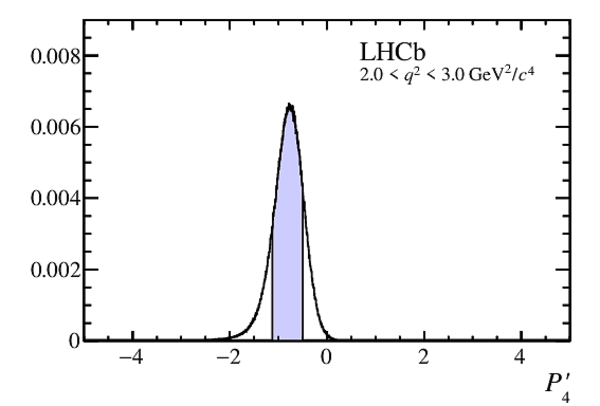
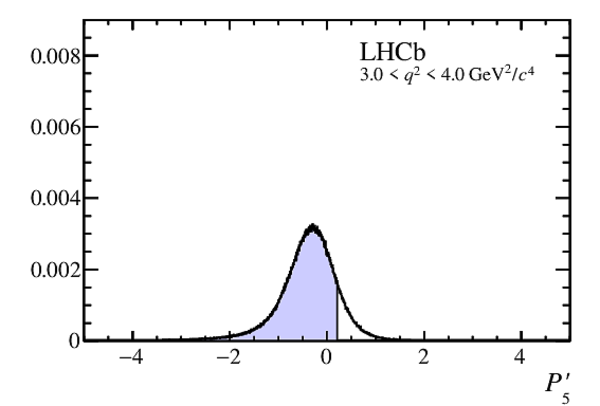
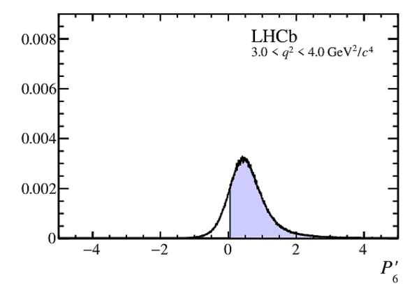
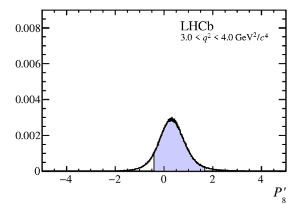
Supplementary Material [file]


![HiDef png [704 KiB]](Directory_LHCb-PAPER-2015-051/hidef_Fig1.png)
![HiDef png [135 KiB]](Directory_LHCb-PAPER-2015-051/hidef_effctl.png)
![HiDef png [145 KiB]](Directory_LHCb-PAPER-2015-051/hidef_effctk.png)
![HiDef png [131 KiB]](Directory_LHCb-PAPER-2015-051/hidef_effphi.png)
![HiDef png [77 KiB]](Directory_LHCb-PAPER-2015-051/hidef_effqsq.png)
![HiDef png [169 KiB]](Directory_LHCb-PAPER-2015-051/hidef_mjpsi.png)
![HiDef png [230 KiB]](Directory_LHCb-PAPER-2015-051/hidef_msignal.png)
![HiDef png [262 KiB]](Directory_LHCb-PAPER-2015-051/hidef_m8.png)
![HiDef png [284 KiB]](Directory_LHCb-PAPER-2015-051/hidef_mkpi8sig.png)
![HiDef png [349 KiB]](Directory_LHCb-PAPER-2015-051/hidef_costhetal8sig.png)
![HiDef png [282 KiB]](Directory_LHCb-PAPER-2015-051/hidef_costhetak8sig.png)
![HiDef png [333 KiB]](Directory_LHCb-PAPER-2015-051/hidef_phi8sig.png)
![HiDef png [306 KiB]](Directory_LHCb-PAPER-2015-051/hidef_projections_amplitudes_ctl_sig.png)
![HiDef png [312 KiB]](Directory_LHCb-PAPER-2015-051/hidef_projections_amplitudes_ctk_sig.png)
![HiDef png [282 KiB]](Directory_LHCb-PAPER-2015-051/hidef_projections_amplitudes_phi_sig.png)
![HiDef png [314 KiB]](Directory_LHCb-PAPER-2015-051/hidef_projections_amplitudes_q2_sig.png)
![HiDef png [84 KiB]](Directory_LHCb-PAPER-2015-051/hidef_FLPad.png)
![HiDef png [78 KiB]](Directory_LHCb-PAPER-2015-051/hidef_AFBPad.png)
![HiDef png [75 KiB]](Directory_LHCb-PAPER-2015-051/hidef_S3Pad.png)
![HiDef png [77 KiB]](Directory_LHCb-PAPER-2015-051/hidef_S4Pad.png)
![HiDef png [75 KiB]](Directory_LHCb-PAPER-2015-051/hidef_S5Pad.png)
![HiDef png [46 KiB]](Directory_LHCb-PAPER-2015-051/hidef_S7Pad.png)
![HiDef png [46 KiB]](Directory_LHCb-PAPER-2015-051/hidef_S8Pad.png)
![HiDef png [46 KiB]](Directory_LHCb-PAPER-2015-051/hidef_S9Pad.png)
![HiDef png [46 KiB]](Directory_LHCb-PAPER-2015-051/hidef_A3Pad.png)
![HiDef png [46 KiB]](Directory_LHCb-PAPER-2015-051/hidef_A4Pad.png)
![HiDef png [46 KiB]](Directory_LHCb-PAPER-2015-051/hidef_A5Pad.png)
![HiDef png [47 KiB]](Directory_LHCb-PAPER-2015-051/hidef_A6Pad.png)
![HiDef png [46 KiB]](Directory_LHCb-PAPER-2015-051/hidef_A7Pad.png)
![HiDef png [47 KiB]](Directory_LHCb-PAPER-2015-051/hidef_A8Pad.png)
![HiDef png [46 KiB]](Directory_LHCb-PAPER-2015-051/hidef_A9Pad.png)
![HiDef png [77 KiB]](Directory_LHCb-PAPER-2015-051/hidef_PBasis_P1Pad.png)
![HiDef png [74 KiB]](Directory_LHCb-PAPER-2015-051/hidef_PBasis_P2Pad.png)
![HiDef png [74 KiB]](Directory_LHCb-PAPER-2015-051/hidef_PBasis_P3Pad.png)
![HiDef png [77 KiB]](Directory_LHCb-PAPER-2015-051/hidef_PBasis_P4pPad.png)
![HiDef png [75 KiB]](Directory_LHCb-PAPER-2015-051/hidef_PBasis_P5pPad.png)
![HiDef png [75 KiB]](Directory_LHCb-PAPER-2015-051/hidef_PBasis_P6pPad.png)
![HiDef png [75 KiB]](Directory_LHCb-PAPER-2015-051/hidef_PBasis_P8pPad.png)
![HiDef png [88 KiB]](Directory_LHCb-PAPER-2015-051/hidef_moments_FLPad.png)
![HiDef png [91 KiB]](Directory_LHCb-PAPER-2015-051/hidef_moments_AFBPad.png)
![HiDef png [85 KiB]](Directory_LHCb-PAPER-2015-051/hidef_moments_S3Pad.png)
![HiDef png [87 KiB]](Directory_LHCb-PAPER-2015-051/hidef_moments_S4Pad.png)
![HiDef png [89 KiB]](Directory_LHCb-PAPER-2015-051/hidef_moments_S5Pad.png)
![HiDef png [54 KiB]](Directory_LHCb-PAPER-2015-051/hidef_moments_S7Pad.png)
![HiDef png [55 KiB]](Directory_LHCb-PAPER-2015-051/hidef_moments_S8Pad.png)
![HiDef png [54 KiB]](Directory_LHCb-PAPER-2015-051/hidef_moments_S9Pad.png)
![HiDef png [54 KiB]](Directory_LHCb-PAPER-2015-051/hidef_moments_A3Pad.png)
![HiDef png [55 KiB]](Directory_LHCb-PAPER-2015-051/hidef_moments_A4Pad.png)
![HiDef png [55 KiB]](Directory_LHCb-PAPER-2015-051/hidef_moments_A5Pad.png)
![HiDef png [55 KiB]](Directory_LHCb-PAPER-2015-051/hidef_moments_A6Pad.png)
![HiDef png [54 KiB]](Directory_LHCb-PAPER-2015-051/hidef_moments_A7Pad.png)
![HiDef png [55 KiB]](Directory_LHCb-PAPER-2015-051/hidef_moments_A8Pad.png)
![HiDef png [54 KiB]](Directory_LHCb-PAPER-2015-051/hidef_moments_A9Pad.png)
![HiDef png [88 KiB]](Directory_LHCb-PAPER-2015-051/hidef_PBasis_Moments_P1Pad.png)
![HiDef png [87 KiB]](Directory_LHCb-PAPER-2015-051/hidef_PBasis_Moments_P2Pad.png)
![HiDef png [84 KiB]](Directory_LHCb-PAPER-2015-051/hidef_PBasis_Moments_P3Pad.png)
![HiDef png [88 KiB]](Directory_LHCb-PAPER-2015-051/hidef_PBasis_Moments_P4pPad.png)
![HiDef png [87 KiB]](Directory_LHCb-PAPER-2015-051/hidef_PBasis_Moments_P5pPad.png)
![HiDef png [84 KiB]](Directory_LHCb-PAPER-2015-051/hidef_PBasis_Moments_P6pPad.png)
![HiDef png [87 KiB]](Directory_LHCb-PAPER-2015-051/hidef_PBasis_Moments_P8pPad.png)
![HiDef png [57 KiB]](Directory_LHCb-PAPER-2015-051/hidef_S6cPad.png)
![HiDef png [107 KiB]](Directory_LHCb-PAPER-2015-051/hidef_amplitudes_S4.png)
![HiDef png [112 KiB]](Directory_LHCb-PAPER-2015-051/hidef_amplitudes_S5.png)
![HiDef png [111 KiB]](Directory_LHCb-PAPER-2015-051/hidef_amplitudes_AFB.png)
![HiDef png [118 KiB]](Directory_LHCb-PAPER-2015-051/hidef_wilsonchi2.png)
![HiDef png [576 KiB]](Directory_LHCb-PAPER-2015-051/hidef_mlogjpsi.png)
![HiDef png [232 KiB]](Directory_LHCb-PAPER-2015-051/hidef_mkpijpsi.png)
![HiDef png [236 KiB]](Directory_LHCb-PAPER-2015-051/hidef_costhetaljpsi.png)
![HiDef png [209 KiB]](Directory_LHCb-PAPER-2015-051/hidef_costhetakjpsi.png)
![HiDef png [222 KiB]](Directory_LHCb-PAPER-2015-051/hidef_phijpsi.png)
![HiDef png [186 KiB]](Directory_LHCb-PAPER-2015-051/hidef_m0.png)
![HiDef png [212 KiB]](Directory_LHCb-PAPER-2015-051/hidef_mkpi0sig.png)
![HiDef png [215 KiB]](Directory_LHCb-PAPER-2015-051/hidef_costhetal0sig.png)
![HiDef png [205 KiB]](Directory_LHCb-PAPER-2015-051/hidef_costhetak0sig.png)
![HiDef png [202 KiB]](Directory_LHCb-PAPER-2015-051/hidef_phi0sig.png)
![HiDef png [227 KiB]](Directory_LHCb-PAPER-2015-051/hidef_m1.png)
![HiDef png [269 KiB]](Directory_LHCb-PAPER-2015-051/hidef_mkpi1sig.png)
![HiDef png [254 KiB]](Directory_LHCb-PAPER-2015-051/hidef_costhetal1sig.png)
![HiDef png [230 KiB]](Directory_LHCb-PAPER-2015-051/hidef_costhetak1sig.png)
![HiDef png [260 KiB]](Directory_LHCb-PAPER-2015-051/hidef_phi1sig.png)
![HiDef png [281 KiB]](Directory_LHCb-PAPER-2015-051/hidef_m2.png)
![HiDef png [293 KiB]](Directory_LHCb-PAPER-2015-051/hidef_mkpi2sig.png)
![HiDef png [308 KiB]](Directory_LHCb-PAPER-2015-051/hidef_costhetal2sig.png)
![HiDef png [268 KiB]](Directory_LHCb-PAPER-2015-051/hidef_costhetak2sig.png)
![HiDef png [306 KiB]](Directory_LHCb-PAPER-2015-051/hidef_phi2sig.png)
![HiDef png [264 KiB]](Directory_LHCb-PAPER-2015-051/hidef_m3.png)
![HiDef png [261 KiB]](Directory_LHCb-PAPER-2015-051/hidef_mkpi3sig.png)
![HiDef png [334 KiB]](Directory_LHCb-PAPER-2015-051/hidef_costhetal3sig.png)
![HiDef png [278 KiB]](Directory_LHCb-PAPER-2015-051/hidef_costhetak3sig.png)
![HiDef png [314 KiB]](Directory_LHCb-PAPER-2015-051/hidef_phi3sig.png)
![HiDef png [261 KiB]](Directory_LHCb-PAPER-2015-051/hidef_m4.png)
![HiDef png [256 KiB]](Directory_LHCb-PAPER-2015-051/hidef_mkpi4sig.png)
![HiDef png [287 KiB]](Directory_LHCb-PAPER-2015-051/hidef_costhetal4sig.png)
![HiDef png [283 KiB]](Directory_LHCb-PAPER-2015-051/hidef_costhetak4sig.png)
![HiDef png [324 KiB]](Directory_LHCb-PAPER-2015-051/hidef_phi4sig.png)
![HiDef png [220 KiB]](Directory_LHCb-PAPER-2015-051/hidef_m5.png)
![HiDef png [217 KiB]](Directory_LHCb-PAPER-2015-051/hidef_mkpi5sig.png)
![HiDef png [225 KiB]](Directory_LHCb-PAPER-2015-051/hidef_costhetal5sig.png)
![HiDef png [240 KiB]](Directory_LHCb-PAPER-2015-051/hidef_costhetak5sig.png)
![HiDef png [235 KiB]](Directory_LHCb-PAPER-2015-051/hidef_phi5sig.png)
![HiDef png [224 KiB]](Directory_LHCb-PAPER-2015-051/hidef_m6.png)
![HiDef png [231 KiB]](Directory_LHCb-PAPER-2015-051/hidef_mkpi6sig.png)
![HiDef png [221 KiB]](Directory_LHCb-PAPER-2015-051/hidef_costhetal6sig.png)
![HiDef png [253 KiB]](Directory_LHCb-PAPER-2015-051/hidef_costhetak6sig.png)
![HiDef png [255 KiB]](Directory_LHCb-PAPER-2015-051/hidef_phi6sig.png)
![HiDef png [238 KiB]](Directory_LHCb-PAPER-2015-051/hidef_m7.png)
![HiDef png [236 KiB]](Directory_LHCb-PAPER-2015-051/hidef_mkpi7sig.png)
![HiDef png [245 KiB]](Directory_LHCb-PAPER-2015-051/hidef_costhetal7sig.png)
![HiDef png [256 KiB]](Directory_LHCb-PAPER-2015-051/hidef_costhetak7sig.png)
![HiDef png [257 KiB]](Directory_LHCb-PAPER-2015-051/hidef_phi7sig.png)
![HiDef png [217 KiB]](Directory_LHCb-PAPER-2015-051/hidef_m9.png)
![HiDef png [226 KiB]](Directory_LHCb-PAPER-2015-051/hidef_mkpi9sig.png)
![HiDef png [218 KiB]](Directory_LHCb-PAPER-2015-051/hidef_costhetal9sig.png)
![HiDef png [236 KiB]](Directory_LHCb-PAPER-2015-051/hidef_costhetak9sig.png)
![HiDef png [232 KiB]](Directory_LHCb-PAPER-2015-051/hidef_phi9sig.png)
![HiDef png [219 KiB]](Directory_LHCb-PAPER-2015-051/hidef_Table_1.png)
![HiDef png [89 KiB]](Directory_LHCb-PAPER-2015-051/hidef_Table_2.png)
![HiDef png [337 KiB]](Directory_LHCb-PAPER-2015-051/hidef_Table_3.png)
![HiDef png [295 KiB]](Directory_LHCb-PAPER-2015-051/hidef_Table_4.png)
![HiDef png [262 KiB]](Directory_LHCb-PAPER-2015-051/hidef_Table_5.png)
![HiDef png [262 KiB]](Directory_LHCb-PAPER-2015-051/hidef_Table_6.png)
![HiDef png [406 KiB]](Directory_LHCb-PAPER-2015-051/hidef_Table_7.png)
![HiDef png [328 KiB]](Directory_LHCb-PAPER-2015-051/hidef_Table_8.png)
![HiDef png [328 KiB]](Directory_LHCb-PAPER-2015-051/hidef_Table_9.png)
![HiDef png [58 KiB]](Directory_LHCb-PAPER-2015-051/hidef_Table_10.png)
![HiDef png [54 KiB]](Directory_LHCb-PAPER-2015-051/hidef_Table_11.png)
![HiDef png [52 KiB]](Directory_LHCb-PAPER-2015-051/hidef_Table_12.png)
![HiDef png [53 KiB]](Directory_LHCb-PAPER-2015-051/hidef_Table_13.png)
![HiDef png [53 KiB]](Directory_LHCb-PAPER-2015-051/hidef_Table_14.png)
![HiDef png [58 KiB]](Directory_LHCb-PAPER-2015-051/hidef_Table_15.png)
![HiDef png [55 KiB]](Directory_LHCb-PAPER-2015-051/hidef_Table_16.png)
![HiDef png [54 KiB]](Directory_LHCb-PAPER-2015-051/hidef_Table_17.png)
![HiDef png [53 KiB]](Directory_LHCb-PAPER-2015-051/hidef_Table_18.png)
![HiDef png [53 KiB]](Directory_LHCb-PAPER-2015-051/hidef_Table_19.png)
![HiDef png [51 KiB]](Directory_LHCb-PAPER-2015-051/hidef_Table_20.png)
![HiDef png [52 KiB]](Directory_LHCb-PAPER-2015-051/hidef_Table_21.png)
![HiDef png [52 KiB]](Directory_LHCb-PAPER-2015-051/hidef_Table_22.png)
![HiDef png [56 KiB]](Directory_LHCb-PAPER-2015-051/hidef_Table_23.png)
![HiDef png [51 KiB]](Directory_LHCb-PAPER-2015-051/hidef_Table_24.png)
![HiDef png [50 KiB]](Directory_LHCb-PAPER-2015-051/hidef_Table_25.png)
![HiDef png [56 KiB]](Directory_LHCb-PAPER-2015-051/hidef_Table_26.png)
![HiDef png [53 KiB]](Directory_LHCb-PAPER-2015-051/hidef_Table_27.png)
![HiDef png [55 KiB]](Directory_LHCb-PAPER-2015-051/hidef_Table_28.png)
![HiDef png [56 KiB]](Directory_LHCb-PAPER-2015-051/hidef_Table_29.png)
![HiDef png [53 KiB]](Directory_LHCb-PAPER-2015-051/hidef_Table_30.png)
![HiDef png [53 KiB]](Directory_LHCb-PAPER-2015-051/hidef_Table_31.png)
![HiDef png [55 KiB]](Directory_LHCb-PAPER-2015-051/hidef_Table_32.png)
![HiDef png [56 KiB]](Directory_LHCb-PAPER-2015-051/hidef_Table_33.png)
![HiDef png [55 KiB]](Directory_LHCb-PAPER-2015-051/hidef_Table_34.png)
![HiDef png [55 KiB]](Directory_LHCb-PAPER-2015-051/hidef_Table_35.png)
![HiDef png [56 KiB]](Directory_LHCb-PAPER-2015-051/hidef_Table_36.png)
![HiDef png [54 KiB]](Directory_LHCb-PAPER-2015-051/hidef_Table_37.png)
![HiDef png [54 KiB]](Directory_LHCb-PAPER-2015-051/hidef_Table_38.png)
![HiDef png [53 KiB]](Directory_LHCb-PAPER-2015-051/hidef_Table_39.png)
![HiDef png [57 KiB]](Directory_LHCb-PAPER-2015-051/hidef_Table_40.png)
![HiDef png [55 KiB]](Directory_LHCb-PAPER-2015-051/hidef_Table_41.png)
![HiDef png [52 KiB]](Directory_LHCb-PAPER-2015-051/hidef_Table_42.png)
![HiDef png [55 KiB]](Directory_LHCb-PAPER-2015-051/hidef_Table_43.png)
![HiDef png [51 KiB]](Directory_LHCb-PAPER-2015-051/hidef_Table_44.png)
![HiDef png [53 KiB]](Directory_LHCb-PAPER-2015-051/hidef_Table_45.png)
![HiDef png [54 KiB]](Directory_LHCb-PAPER-2015-051/hidef_Table_46.png)
![HiDef png [54 KiB]](Directory_LHCb-PAPER-2015-051/hidef_Table_47.png)
![HiDef png [54 KiB]](Directory_LHCb-PAPER-2015-051/hidef_Table_48.png)
![HiDef png [54 KiB]](Directory_LHCb-PAPER-2015-051/hidef_Table_49.png)
![HiDef png [55 KiB]](Directory_LHCb-PAPER-2015-051/hidef_Table_50.png)
![HiDef png [54 KiB]](Directory_LHCb-PAPER-2015-051/hidef_Table_51.png)
![HiDef png [55 KiB]](Directory_LHCb-PAPER-2015-051/hidef_Table_52.png)
![HiDef png [54 KiB]](Directory_LHCb-PAPER-2015-051/hidef_Table_53.png)
![HiDef png [53 KiB]](Directory_LHCb-PAPER-2015-051/hidef_Table_54.png)
![HiDef png [51 KiB]](Directory_LHCb-PAPER-2015-051/hidef_Table_55.png)
![HiDef png [49 KiB]](Directory_LHCb-PAPER-2015-051/hidef_Table_56.png)
![HiDef png [50 KiB]](Directory_LHCb-PAPER-2015-051/hidef_Table_57.png)
![HiDef png [53 KiB]](Directory_LHCb-PAPER-2015-051/hidef_Table_58.png)
![HiDef png [49 KiB]](Directory_LHCb-PAPER-2015-051/hidef_Table_59.png)
![HiDef png [49 KiB]](Directory_LHCb-PAPER-2015-051/hidef_Table_60.png)
![HiDef png [50 KiB]](Directory_LHCb-PAPER-2015-051/hidef_Table_61.png)
![HiDef png [48 KiB]](Directory_LHCb-PAPER-2015-051/hidef_Table_62.png)
![HiDef png [50 KiB]](Directory_LHCb-PAPER-2015-051/hidef_Table_63.png)
![HiDef png [48 KiB]](Directory_LHCb-PAPER-2015-051/hidef_Table_64.png)
![HiDef png [50 KiB]](Directory_LHCb-PAPER-2015-051/hidef_Table_65.png)
![HiDef png [50 KiB]](Directory_LHCb-PAPER-2015-051/hidef_Table_66.png)
![HiDef png [50 KiB]](Directory_LHCb-PAPER-2015-051/hidef_Table_67.png)
![HiDef png [49 KiB]](Directory_LHCb-PAPER-2015-051/hidef_Table_68.png)
![HiDef png [49 KiB]](Directory_LHCb-PAPER-2015-051/hidef_Table_69.png)
![HiDef png [55 KiB]](Directory_LHCb-PAPER-2015-051/hidef_Table_70.png)
![HiDef png [53 KiB]](Directory_LHCb-PAPER-2015-051/hidef_Table_71.png)
![HiDef png [54 KiB]](Directory_LHCb-PAPER-2015-051/hidef_Table_72.png)
![HiDef png [54 KiB]](Directory_LHCb-PAPER-2015-051/hidef_Table_73.png)
![HiDef png [54 KiB]](Directory_LHCb-PAPER-2015-051/hidef_Table_74.png)
![HiDef png [52 KiB]](Directory_LHCb-PAPER-2015-051/hidef_Table_75.png)
![HiDef png [54 KiB]](Directory_LHCb-PAPER-2015-051/hidef_Table_76.png)
![HiDef png [53 KiB]](Directory_LHCb-PAPER-2015-051/hidef_Table_77.png)
![HiDef png [53 KiB]](Directory_LHCb-PAPER-2015-051/hidef_Table_78.png)
![HiDef png [53 KiB]](Directory_LHCb-PAPER-2015-051/hidef_Table_79.png)
![HiDef png [56 KiB]](Directory_LHCb-PAPER-2015-051/hidef_Table_80.png)
![HiDef png [57 KiB]](Directory_LHCb-PAPER-2015-051/hidef_Table_81.png)
![HiDef png [55 KiB]](Directory_LHCb-PAPER-2015-051/hidef_Table_82.png)
![HiDef png [56 KiB]](Directory_LHCb-PAPER-2015-051/hidef_Table_83.png)
![HiDef png [56 KiB]](Directory_LHCb-PAPER-2015-051/hidef_Table_84.png)
![HiDef png [101 KiB]](Directory_LHCb-PAPER-2015-051/supplementary/hidef_Fig10aS.png)
![HiDef png [101 KiB]](Directory_LHCb-PAPER-2015-051/supplementary/hidef_Fig10bS.png)
![HiDef png [103 KiB]](Directory_LHCb-PAPER-2015-051/supplementary/hidef_Fig10cS.png)
![HiDef png [106 KiB]](Directory_LHCb-PAPER-2015-051/supplementary/hidef_Fig10dS.png)
![HiDef png [105 KiB]](Directory_LHCb-PAPER-2015-051/supplementary/hidef_Fig10eS.png)
![HiDef png [103 KiB]](Directory_LHCb-PAPER-2015-051/supplementary/hidef_Fig10fS.png)
![HiDef png [104 KiB]](Directory_LHCb-PAPER-2015-051/supplementary/hidef_Fig10gS.png)
![HiDef png [103 KiB]](Directory_LHCb-PAPER-2015-051/supplementary/hidef_Fig10hS.png)
![HiDef png [107 KiB]](Directory_LHCb-PAPER-2015-051/supplementary/hidef_Fig11aS.png)
![HiDef png [110 KiB]](Directory_LHCb-PAPER-2015-051/supplementary/hidef_Fig11bS.png)
![HiDef png [106 KiB]](Directory_LHCb-PAPER-2015-051/supplementary/hidef_Fig11cS.png)
![HiDef png [111 KiB]](Directory_LHCb-PAPER-2015-051/supplementary/hidef_Fig11dS.png)
![HiDef png [107 KiB]](Directory_LHCb-PAPER-2015-051/supplementary/hidef_Fig11eS.png)
![HiDef png [111 KiB]](Directory_LHCb-PAPER-2015-051/supplementary/hidef_Fig11fS.png)
![HiDef png [108 KiB]](Directory_LHCb-PAPER-2015-051/supplementary/hidef_Fig11gS.png)
![HiDef png [120 KiB]](Directory_LHCb-PAPER-2015-051/supplementary/hidef_Fig12aS.png)
![HiDef png [121 KiB]](Directory_LHCb-PAPER-2015-051/supplementary/hidef_Fig12bS.png)
![HiDef png [120 KiB]](Directory_LHCb-PAPER-2015-051/supplementary/hidef_Fig12cS.png)
![HiDef png [121 KiB]](Directory_LHCb-PAPER-2015-051/supplementary/hidef_Fig12dS.png)
![HiDef png [117 KiB]](Directory_LHCb-PAPER-2015-051/supplementary/hidef_Fig12eS.png)
![HiDef png [122 KiB]](Directory_LHCb-PAPER-2015-051/supplementary/hidef_Fig12fS.png)
![HiDef png [119 KiB]](Directory_LHCb-PAPER-2015-051/supplementary/hidef_Fig12gS.png)
![HiDef png [121 KiB]](Directory_LHCb-PAPER-2015-051/supplementary/hidef_Fig13aS.png)
![HiDef png [125 KiB]](Directory_LHCb-PAPER-2015-051/supplementary/hidef_Fig13bS.png)
![HiDef png [123 KiB]](Directory_LHCb-PAPER-2015-051/supplementary/hidef_Fig13cS.png)
![HiDef png [123 KiB]](Directory_LHCb-PAPER-2015-051/supplementary/hidef_Fig13dS.png)
![HiDef png [123 KiB]](Directory_LHCb-PAPER-2015-051/supplementary/hidef_Fig13eS.png)
![HiDef png [125 KiB]](Directory_LHCb-PAPER-2015-051/supplementary/hidef_Fig13fS.png)
![HiDef png [124 KiB]](Directory_LHCb-PAPER-2015-051/supplementary/hidef_Fig13gS.png)
![HiDef png [117 KiB]](Directory_LHCb-PAPER-2015-051/supplementary/hidef_Fig14aS.png)
![HiDef png [115 KiB]](Directory_LHCb-PAPER-2015-051/supplementary/hidef_Fig14bS.png)
![HiDef png [113 KiB]](Directory_LHCb-PAPER-2015-051/supplementary/hidef_Fig14cS.png)
![HiDef png [121 KiB]](Directory_LHCb-PAPER-2015-051/supplementary/hidef_Fig14dS.png)
![HiDef png [115 KiB]](Directory_LHCb-PAPER-2015-051/supplementary/hidef_Fig14eS.png)
![HiDef png [115 KiB]](Directory_LHCb-PAPER-2015-051/supplementary/hidef_Fig14fS.png)
![HiDef png [117 KiB]](Directory_LHCb-PAPER-2015-051/supplementary/hidef_Fig14gS.png)
![HiDef png [111 KiB]](Directory_LHCb-PAPER-2015-051/supplementary/hidef_Fig15aS.png)
![HiDef png [110 KiB]](Directory_LHCb-PAPER-2015-051/supplementary/hidef_Fig15bS.png)
![HiDef png [108 KiB]](Directory_LHCb-PAPER-2015-051/supplementary/hidef_Fig15cS.png)
![HiDef png [118 KiB]](Directory_LHCb-PAPER-2015-051/supplementary/hidef_Fig15dS.png)
![HiDef png [106 KiB]](Directory_LHCb-PAPER-2015-051/supplementary/hidef_Fig15eS.png)
![HiDef png [109 KiB]](Directory_LHCb-PAPER-2015-051/supplementary/hidef_Fig15fS.png)
![HiDef png [110 KiB]](Directory_LHCb-PAPER-2015-051/supplementary/hidef_Fig15gS.png)
![HiDef png [112 KiB]](Directory_LHCb-PAPER-2015-051/supplementary/hidef_Fig16aS.png)
![HiDef png [111 KiB]](Directory_LHCb-PAPER-2015-051/supplementary/hidef_Fig16bS.png)
![HiDef png [109 KiB]](Directory_LHCb-PAPER-2015-051/supplementary/hidef_Fig16cS.png)
![HiDef png [119 KiB]](Directory_LHCb-PAPER-2015-051/supplementary/hidef_Fig16dS.png)
![HiDef png [109 KiB]](Directory_LHCb-PAPER-2015-051/supplementary/hidef_Fig16eS.png)
![HiDef png [108 KiB]](Directory_LHCb-PAPER-2015-051/supplementary/hidef_Fig16fS.png)
![HiDef png [106 KiB]](Directory_LHCb-PAPER-2015-051/supplementary/hidef_Fig16gS.png)
![HiDef png [105 KiB]](Directory_LHCb-PAPER-2015-051/supplementary/hidef_Fig17aS.png)
![HiDef png [106 KiB]](Directory_LHCb-PAPER-2015-051/supplementary/hidef_Fig17bS.png)
![HiDef png [107 KiB]](Directory_LHCb-PAPER-2015-051/supplementary/hidef_Fig17cS.png)
![HiDef png [117 KiB]](Directory_LHCb-PAPER-2015-051/supplementary/hidef_Fig17dS.png)
![HiDef png [105 KiB]](Directory_LHCb-PAPER-2015-051/supplementary/hidef_Fig17eS.png)
![HiDef png [106 KiB]](Directory_LHCb-PAPER-2015-051/supplementary/hidef_Fig17fS.png)
![HiDef png [105 KiB]](Directory_LHCb-PAPER-2015-051/supplementary/hidef_Fig17gS.png)
![HiDef png [111 KiB]](Directory_LHCb-PAPER-2015-051/supplementary/hidef_Fig18aS.png)
![HiDef png [110 KiB]](Directory_LHCb-PAPER-2015-051/supplementary/hidef_Fig18bS.png)
![HiDef png [110 KiB]](Directory_LHCb-PAPER-2015-051/supplementary/hidef_Fig18cS.png)
![HiDef png [120 KiB]](Directory_LHCb-PAPER-2015-051/supplementary/hidef_Fig18dS.png)
![HiDef png [108 KiB]](Directory_LHCb-PAPER-2015-051/supplementary/hidef_Fig18eS.png)
![HiDef png [110 KiB]](Directory_LHCb-PAPER-2015-051/supplementary/hidef_Fig18fS.png)
![HiDef png [109 KiB]](Directory_LHCb-PAPER-2015-051/supplementary/hidef_Fig18gS.png)
![HiDef png [101 KiB]](Directory_LHCb-PAPER-2015-051/supplementary/hidef_Fig19aS.png)
![HiDef png [112 KiB]](Directory_LHCb-PAPER-2015-051/supplementary/hidef_Fig19bS.png)
![HiDef png [105 KiB]](Directory_LHCb-PAPER-2015-051/supplementary/hidef_Fig19cS.png)
![HiDef png [117 KiB]](Directory_LHCb-PAPER-2015-051/supplementary/hidef_Fig19dS.png)
![HiDef png [108 KiB]](Directory_LHCb-PAPER-2015-051/supplementary/hidef_Fig19eS.png)
![HiDef png [114 KiB]](Directory_LHCb-PAPER-2015-051/supplementary/hidef_Fig19fS.png)
![HiDef png [101 KiB]](Directory_LHCb-PAPER-2015-051/supplementary/hidef_Fig19gS.png)
![HiDef png [105 KiB]](Directory_LHCb-PAPER-2015-051/supplementary/hidef_Fig1aS.png)
![HiDef png [108 KiB]](Directory_LHCb-PAPER-2015-051/supplementary/hidef_Fig1bS.png)
![HiDef png [107 KiB]](Directory_LHCb-PAPER-2015-051/supplementary/hidef_Fig1cS.png)
![HiDef png [109 KiB]](Directory_LHCb-PAPER-2015-051/supplementary/hidef_Fig1dS.png)
![HiDef png [107 KiB]](Directory_LHCb-PAPER-2015-051/supplementary/hidef_Fig1eS.png)
![HiDef png [107 KiB]](Directory_LHCb-PAPER-2015-051/supplementary/hidef_Fig1fS.png)
![HiDef png [111 KiB]](Directory_LHCb-PAPER-2015-051/supplementary/hidef_Fig1gS.png)
![HiDef png [107 KiB]](Directory_LHCb-PAPER-2015-051/supplementary/hidef_Fig1hS.png)
![HiDef png [104 KiB]](Directory_LHCb-PAPER-2015-051/supplementary/hidef_Fig20aS.png)
![HiDef png [105 KiB]](Directory_LHCb-PAPER-2015-051/supplementary/hidef_Fig20bS.png)
![HiDef png [105 KiB]](Directory_LHCb-PAPER-2015-051/supplementary/hidef_Fig20cS.png)
![HiDef png [117 KiB]](Directory_LHCb-PAPER-2015-051/supplementary/hidef_Fig20dS.png)
![HiDef png [103 KiB]](Directory_LHCb-PAPER-2015-051/supplementary/hidef_Fig20eS.png)
![HiDef png [104 KiB]](Directory_LHCb-PAPER-2015-051/supplementary/hidef_Fig20fS.png)
![HiDef png [104 KiB]](Directory_LHCb-PAPER-2015-051/supplementary/hidef_Fig20gS.png)
![HiDef png [108 KiB]](Directory_LHCb-PAPER-2015-051/supplementary/hidef_Fig21aS.png)
![HiDef png [98 KiB]](Directory_LHCb-PAPER-2015-051/supplementary/hidef_Fig21bS.png)
![HiDef png [100 KiB]](Directory_LHCb-PAPER-2015-051/supplementary/hidef_Fig21cS.png)
![HiDef png [110 KiB]](Directory_LHCb-PAPER-2015-051/supplementary/hidef_Fig21dS.png)
![HiDef png [106 KiB]](Directory_LHCb-PAPER-2015-051/supplementary/hidef_Fig21eS.png)
![HiDef png [106 KiB]](Directory_LHCb-PAPER-2015-051/supplementary/hidef_Fig21fS.png)
![HiDef png [110 KiB]](Directory_LHCb-PAPER-2015-051/supplementary/hidef_Fig21gS.png)
![HiDef png [115 KiB]](Directory_LHCb-PAPER-2015-051/supplementary/hidef_Fig22aS.png)
![HiDef png [114 KiB]](Directory_LHCb-PAPER-2015-051/supplementary/hidef_Fig22bS.png)
![HiDef png [121 KiB]](Directory_LHCb-PAPER-2015-051/supplementary/hidef_Fig22cS.png)
![HiDef png [119 KiB]](Directory_LHCb-PAPER-2015-051/supplementary/hidef_Fig22dS.png)
![HiDef png [117 KiB]](Directory_LHCb-PAPER-2015-051/supplementary/hidef_Fig22eS.png)
![HiDef png [116 KiB]](Directory_LHCb-PAPER-2015-051/supplementary/hidef_Fig22fS.png)
![HiDef png [120 KiB]](Directory_LHCb-PAPER-2015-051/supplementary/hidef_Fig22gS.png)
![HiDef png [100 KiB]](Directory_LHCb-PAPER-2015-051/supplementary/hidef_Fig23aS.png)
![HiDef png [110 KiB]](Directory_LHCb-PAPER-2015-051/supplementary/hidef_Fig23bS.png)
![HiDef png [106 KiB]](Directory_LHCb-PAPER-2015-051/supplementary/hidef_Fig23cS.png)
![HiDef png [109 KiB]](Directory_LHCb-PAPER-2015-051/supplementary/hidef_Fig23dS.png)
![HiDef png [124 KiB]](Directory_LHCb-PAPER-2015-051/supplementary/hidef_Fig23eS.png)
![HiDef png [119 KiB]](Directory_LHCb-PAPER-2015-051/supplementary/hidef_Fig23fS.png)
![HiDef png [125 KiB]](Directory_LHCb-PAPER-2015-051/supplementary/hidef_Fig23gS.png)
![HiDef png [121 KiB]](Directory_LHCb-PAPER-2015-051/supplementary/hidef_Fig24aS.png)
![HiDef png [99 KiB]](Directory_LHCb-PAPER-2015-051/supplementary/hidef_Fig24bS.png)
![HiDef png [114 KiB]](Directory_LHCb-PAPER-2015-051/supplementary/hidef_Fig24cS.png)
![HiDef png [111 KiB]](Directory_LHCb-PAPER-2015-051/supplementary/hidef_Fig24dS.png)
![HiDef png [108 KiB]](Directory_LHCb-PAPER-2015-051/supplementary/hidef_Fig24eS.png)
![HiDef png [109 KiB]](Directory_LHCb-PAPER-2015-051/supplementary/hidef_Fig24fS.png)
![HiDef png [113 KiB]](Directory_LHCb-PAPER-2015-051/supplementary/hidef_Fig24gS.png)
![HiDef png [119 KiB]](Directory_LHCb-PAPER-2015-051/supplementary/hidef_Fig25aS.png)
![HiDef png [96 KiB]](Directory_LHCb-PAPER-2015-051/supplementary/hidef_Fig25bS.png)
![HiDef png [109 KiB]](Directory_LHCb-PAPER-2015-051/supplementary/hidef_Fig25cS.png)
![HiDef png [108 KiB]](Directory_LHCb-PAPER-2015-051/supplementary/hidef_Fig25dS.png)
![HiDef png [105 KiB]](Directory_LHCb-PAPER-2015-051/supplementary/hidef_Fig25eS.png)
![HiDef png [105 KiB]](Directory_LHCb-PAPER-2015-051/supplementary/hidef_Fig25fS.png)
![HiDef png [107 KiB]](Directory_LHCb-PAPER-2015-051/supplementary/hidef_Fig25gS.png)
![HiDef png [113 KiB]](Directory_LHCb-PAPER-2015-051/supplementary/hidef_Fig26aS.png)
![HiDef png [102 KiB]](Directory_LHCb-PAPER-2015-051/supplementary/hidef_Fig26bS.png)
![HiDef png [113 KiB]](Directory_LHCb-PAPER-2015-051/supplementary/hidef_Fig26cS.png)
![HiDef png [117 KiB]](Directory_LHCb-PAPER-2015-051/supplementary/hidef_Fig26dS.png)
![HiDef png [115 KiB]](Directory_LHCb-PAPER-2015-051/supplementary/hidef_Fig26eS.png)
![HiDef png [114 KiB]](Directory_LHCb-PAPER-2015-051/supplementary/hidef_Fig26fS.png)
![HiDef png [114 KiB]](Directory_LHCb-PAPER-2015-051/supplementary/hidef_Fig26gS.png)
![HiDef png [111 KiB]](Directory_LHCb-PAPER-2015-051/supplementary/hidef_Fig27aS.png)
![HiDef png [97 KiB]](Directory_LHCb-PAPER-2015-051/supplementary/hidef_Fig27bS.png)
![HiDef png [102 KiB]](Directory_LHCb-PAPER-2015-051/supplementary/hidef_Fig27cS.png)
![HiDef png [115 KiB]](Directory_LHCb-PAPER-2015-051/supplementary/hidef_Fig27dS.png)
![HiDef png [111 KiB]](Directory_LHCb-PAPER-2015-051/supplementary/hidef_Fig27eS.png)
![HiDef png [105 KiB]](Directory_LHCb-PAPER-2015-051/supplementary/hidef_Fig27fS.png)
![HiDef png [111 KiB]](Directory_LHCb-PAPER-2015-051/supplementary/hidef_Fig27gS.png)
![HiDef png [117 KiB]](Directory_LHCb-PAPER-2015-051/supplementary/hidef_Fig28aS.png)
![HiDef png [95 KiB]](Directory_LHCb-PAPER-2015-051/supplementary/hidef_Fig28bS.png)
![HiDef png [110 KiB]](Directory_LHCb-PAPER-2015-051/supplementary/hidef_Fig28cS.png)
![HiDef png [116 KiB]](Directory_LHCb-PAPER-2015-051/supplementary/hidef_Fig28dS.png)
![HiDef png [116 KiB]](Directory_LHCb-PAPER-2015-051/supplementary/hidef_Fig28eS.png)
![HiDef png [112 KiB]](Directory_LHCb-PAPER-2015-051/supplementary/hidef_Fig28fS.png)
![HiDef png [111 KiB]](Directory_LHCb-PAPER-2015-051/supplementary/hidef_Fig28gS.png)
![HiDef png [112 KiB]](Directory_LHCb-PAPER-2015-051/supplementary/hidef_Fig29aS.png)
![HiDef png [102 KiB]](Directory_LHCb-PAPER-2015-051/supplementary/hidef_Fig29bS.png)
![HiDef png [105 KiB]](Directory_LHCb-PAPER-2015-051/supplementary/hidef_Fig29cS.png)
![HiDef png [111 KiB]](Directory_LHCb-PAPER-2015-051/supplementary/hidef_Fig29dS.png)
![HiDef png [106 KiB]](Directory_LHCb-PAPER-2015-051/supplementary/hidef_Fig29eS.png)
![HiDef png [106 KiB]](Directory_LHCb-PAPER-2015-051/supplementary/hidef_Fig29fS.png)
![HiDef png [111 KiB]](Directory_LHCb-PAPER-2015-051/supplementary/hidef_Fig29gS.png)
![HiDef png [119 KiB]](Directory_LHCb-PAPER-2015-051/supplementary/hidef_Fig2aS.png)
![HiDef png [119 KiB]](Directory_LHCb-PAPER-2015-051/supplementary/hidef_Fig2bS.png)
![HiDef png [120 KiB]](Directory_LHCb-PAPER-2015-051/supplementary/hidef_Fig2cS.png)
![HiDef png [122 KiB]](Directory_LHCb-PAPER-2015-051/supplementary/hidef_Fig2dS.png)
![HiDef png [119 KiB]](Directory_LHCb-PAPER-2015-051/supplementary/hidef_Fig2eS.png)
![HiDef png [119 KiB]](Directory_LHCb-PAPER-2015-051/supplementary/hidef_Fig2fS.png)
![HiDef png [122 KiB]](Directory_LHCb-PAPER-2015-051/supplementary/hidef_Fig2gS.png)
![HiDef png [120 KiB]](Directory_LHCb-PAPER-2015-051/supplementary/hidef_Fig2hS.png)
![HiDef png [101 KiB]](Directory_LHCb-PAPER-2015-051/supplementary/hidef_Fig30aS.png)
![HiDef png [92 KiB]](Directory_LHCb-PAPER-2015-051/supplementary/hidef_Fig30bS.png)
![HiDef png [98 KiB]](Directory_LHCb-PAPER-2015-051/supplementary/hidef_Fig30cS.png)
![HiDef png [104 KiB]](Directory_LHCb-PAPER-2015-051/supplementary/hidef_Fig30dS.png)
![HiDef png [101 KiB]](Directory_LHCb-PAPER-2015-051/supplementary/hidef_Fig30eS.png)
![HiDef png [100 KiB]](Directory_LHCb-PAPER-2015-051/supplementary/hidef_Fig30fS.png)
![HiDef png [101 KiB]](Directory_LHCb-PAPER-2015-051/supplementary/hidef_Fig30gS.png)
![HiDef png [100 KiB]](Directory_LHCb-PAPER-2015-051/supplementary/hidef_Fig31aS.png)
![HiDef png [91 KiB]](Directory_LHCb-PAPER-2015-051/supplementary/hidef_Fig31bS.png)
![HiDef png [92 KiB]](Directory_LHCb-PAPER-2015-051/supplementary/hidef_Fig31cS.png)
![HiDef png [90 KiB]](Directory_LHCb-PAPER-2015-051/supplementary/hidef_Fig31dS.png)
![HiDef png [91 KiB]](Directory_LHCb-PAPER-2015-051/supplementary/hidef_Fig31eS.png)
![HiDef png [91 KiB]](Directory_LHCb-PAPER-2015-051/supplementary/hidef_Fig31fS.png)
![HiDef png [92 KiB]](Directory_LHCb-PAPER-2015-051/supplementary/hidef_Fig31gS.png)
![HiDef png [91 KiB]](Directory_LHCb-PAPER-2015-051/supplementary/hidef_Fig31hS.png)
![HiDef png [91 KiB]](Directory_LHCb-PAPER-2015-051/supplementary/hidef_Fig31iS.png)
![HiDef png [99 KiB]](Directory_LHCb-PAPER-2015-051/supplementary/hidef_Fig32aS.png)
![HiDef png [88 KiB]](Directory_LHCb-PAPER-2015-051/supplementary/hidef_Fig32bS.png)
![HiDef png [88 KiB]](Directory_LHCb-PAPER-2015-051/supplementary/hidef_Fig32cS.png)
![HiDef png [89 KiB]](Directory_LHCb-PAPER-2015-051/supplementary/hidef_Fig32dS.png)
![HiDef png [89 KiB]](Directory_LHCb-PAPER-2015-051/supplementary/hidef_Fig32eS.png)
![HiDef png [93 KiB]](Directory_LHCb-PAPER-2015-051/supplementary/hidef_Fig32fS.png)
![HiDef png [88 KiB]](Directory_LHCb-PAPER-2015-051/supplementary/hidef_Fig32gS.png)
![HiDef png [89 KiB]](Directory_LHCb-PAPER-2015-051/supplementary/hidef_Fig32hS.png)
![HiDef png [88 KiB]](Directory_LHCb-PAPER-2015-051/supplementary/hidef_Fig32iS.png)
![HiDef png [100 KiB]](Directory_LHCb-PAPER-2015-051/supplementary/hidef_Fig33aS.png)
![HiDef png [91 KiB]](Directory_LHCb-PAPER-2015-051/supplementary/hidef_Fig33bS.png)
![HiDef png [88 KiB]](Directory_LHCb-PAPER-2015-051/supplementary/hidef_Fig33cS.png)
![HiDef png [88 KiB]](Directory_LHCb-PAPER-2015-051/supplementary/hidef_Fig33dS.png)
![HiDef png [88 KiB]](Directory_LHCb-PAPER-2015-051/supplementary/hidef_Fig33eS.png)
![HiDef png [94 KiB]](Directory_LHCb-PAPER-2015-051/supplementary/hidef_Fig33fS.png)
![HiDef png [89 KiB]](Directory_LHCb-PAPER-2015-051/supplementary/hidef_Fig33gS.png)
![HiDef png [89 KiB]](Directory_LHCb-PAPER-2015-051/supplementary/hidef_Fig33hS.png)
![HiDef png [89 KiB]](Directory_LHCb-PAPER-2015-051/supplementary/hidef_Fig33iS.png)
![HiDef png [95 KiB]](Directory_LHCb-PAPER-2015-051/supplementary/hidef_Fig34aS.png)
![HiDef png [90 KiB]](Directory_LHCb-PAPER-2015-051/supplementary/hidef_Fig34bS.png)
![HiDef png [89 KiB]](Directory_LHCb-PAPER-2015-051/supplementary/hidef_Fig34cS.png)
![HiDef png [91 KiB]](Directory_LHCb-PAPER-2015-051/supplementary/hidef_Fig34dS.png)
![HiDef png [90 KiB]](Directory_LHCb-PAPER-2015-051/supplementary/hidef_Fig34eS.png)
![HiDef png [97 KiB]](Directory_LHCb-PAPER-2015-051/supplementary/hidef_Fig34fS.png)
![HiDef png [89 KiB]](Directory_LHCb-PAPER-2015-051/supplementary/hidef_Fig34gS.png)
![HiDef png [90 KiB]](Directory_LHCb-PAPER-2015-051/supplementary/hidef_Fig34hS.png)
![HiDef png [88 KiB]](Directory_LHCb-PAPER-2015-051/supplementary/hidef_Fig34iS.png)
![HiDef png [95 KiB]](Directory_LHCb-PAPER-2015-051/supplementary/hidef_Fig35aS.png)
![HiDef png [91 KiB]](Directory_LHCb-PAPER-2015-051/supplementary/hidef_Fig35bS.png)
![HiDef png [88 KiB]](Directory_LHCb-PAPER-2015-051/supplementary/hidef_Fig35cS.png)
![HiDef png [89 KiB]](Directory_LHCb-PAPER-2015-051/supplementary/hidef_Fig35dS.png)
![HiDef png [89 KiB]](Directory_LHCb-PAPER-2015-051/supplementary/hidef_Fig35eS.png)
![HiDef png [93 KiB]](Directory_LHCb-PAPER-2015-051/supplementary/hidef_Fig35fS.png)
![HiDef png [89 KiB]](Directory_LHCb-PAPER-2015-051/supplementary/hidef_Fig35gS.png)
![HiDef png [89 KiB]](Directory_LHCb-PAPER-2015-051/supplementary/hidef_Fig35hS.png)
![HiDef png [88 KiB]](Directory_LHCb-PAPER-2015-051/supplementary/hidef_Fig35iS.png)
![HiDef png [102 KiB]](Directory_LHCb-PAPER-2015-051/supplementary/hidef_Fig36aS.png)
![HiDef png [91 KiB]](Directory_LHCb-PAPER-2015-051/supplementary/hidef_Fig36bS.png)
![HiDef png [88 KiB]](Directory_LHCb-PAPER-2015-051/supplementary/hidef_Fig36cS.png)
![HiDef png [90 KiB]](Directory_LHCb-PAPER-2015-051/supplementary/hidef_Fig36dS.png)
![HiDef png [89 KiB]](Directory_LHCb-PAPER-2015-051/supplementary/hidef_Fig36eS.png)
![HiDef png [94 KiB]](Directory_LHCb-PAPER-2015-051/supplementary/hidef_Fig36fS.png)
![HiDef png [89 KiB]](Directory_LHCb-PAPER-2015-051/supplementary/hidef_Fig36gS.png)
![HiDef png [90 KiB]](Directory_LHCb-PAPER-2015-051/supplementary/hidef_Fig36hS.png)
![HiDef png [89 KiB]](Directory_LHCb-PAPER-2015-051/supplementary/hidef_Fig36iS.png)
![HiDef png [99 KiB]](Directory_LHCb-PAPER-2015-051/supplementary/hidef_Fig37aS.png)
![HiDef png [91 KiB]](Directory_LHCb-PAPER-2015-051/supplementary/hidef_Fig37bS.png)
![HiDef png [89 KiB]](Directory_LHCb-PAPER-2015-051/supplementary/hidef_Fig37cS.png)
![HiDef png [89 KiB]](Directory_LHCb-PAPER-2015-051/supplementary/hidef_Fig37dS.png)
![HiDef png [89 KiB]](Directory_LHCb-PAPER-2015-051/supplementary/hidef_Fig37eS.png)
![HiDef png [92 KiB]](Directory_LHCb-PAPER-2015-051/supplementary/hidef_Fig37fS.png)
![HiDef png [88 KiB]](Directory_LHCb-PAPER-2015-051/supplementary/hidef_Fig37gS.png)
![HiDef png [89 KiB]](Directory_LHCb-PAPER-2015-051/supplementary/hidef_Fig37hS.png)
![HiDef png [90 KiB]](Directory_LHCb-PAPER-2015-051/supplementary/hidef_Fig37iS.png)
![HiDef png [100 KiB]](Directory_LHCb-PAPER-2015-051/supplementary/hidef_Fig38aS.png)
![HiDef png [91 KiB]](Directory_LHCb-PAPER-2015-051/supplementary/hidef_Fig38bS.png)
![HiDef png [89 KiB]](Directory_LHCb-PAPER-2015-051/supplementary/hidef_Fig38cS.png)
![HiDef png [88 KiB]](Directory_LHCb-PAPER-2015-051/supplementary/hidef_Fig38dS.png)
![HiDef png [89 KiB]](Directory_LHCb-PAPER-2015-051/supplementary/hidef_Fig38eS.png)
![HiDef png [92 KiB]](Directory_LHCb-PAPER-2015-051/supplementary/hidef_Fig38fS.png)
![HiDef png [89 KiB]](Directory_LHCb-PAPER-2015-051/supplementary/hidef_Fig38gS.png)
![HiDef png [89 KiB]](Directory_LHCb-PAPER-2015-051/supplementary/hidef_Fig38hS.png)
![HiDef png [89 KiB]](Directory_LHCb-PAPER-2015-051/supplementary/hidef_Fig38iS.png)
![HiDef png [99 KiB]](Directory_LHCb-PAPER-2015-051/supplementary/hidef_Fig39aS.png)
![HiDef png [90 KiB]](Directory_LHCb-PAPER-2015-051/supplementary/hidef_Fig39bS.png)
![HiDef png [89 KiB]](Directory_LHCb-PAPER-2015-051/supplementary/hidef_Fig39cS.png)
![HiDef png [89 KiB]](Directory_LHCb-PAPER-2015-051/supplementary/hidef_Fig39dS.png)
![HiDef png [89 KiB]](Directory_LHCb-PAPER-2015-051/supplementary/hidef_Fig39eS.png)
![HiDef png [91 KiB]](Directory_LHCb-PAPER-2015-051/supplementary/hidef_Fig39fS.png)
![HiDef png [88 KiB]](Directory_LHCb-PAPER-2015-051/supplementary/hidef_Fig39gS.png)
![HiDef png [88 KiB]](Directory_LHCb-PAPER-2015-051/supplementary/hidef_Fig39hS.png)
![HiDef png [89 KiB]](Directory_LHCb-PAPER-2015-051/supplementary/hidef_Fig39iS.png)
![HiDef png [116 KiB]](Directory_LHCb-PAPER-2015-051/supplementary/hidef_Fig3aS.png)
![HiDef png [121 KiB]](Directory_LHCb-PAPER-2015-051/supplementary/hidef_Fig3bS.png)
![HiDef png [121 KiB]](Directory_LHCb-PAPER-2015-051/supplementary/hidef_Fig3cS.png)
![HiDef png [122 KiB]](Directory_LHCb-PAPER-2015-051/supplementary/hidef_Fig3dS.png)
![HiDef png [122 KiB]](Directory_LHCb-PAPER-2015-051/supplementary/hidef_Fig3eS.png)
![HiDef png [124 KiB]](Directory_LHCb-PAPER-2015-051/supplementary/hidef_Fig3fS.png)
![HiDef png [127 KiB]](Directory_LHCb-PAPER-2015-051/supplementary/hidef_Fig3gS.png)
![HiDef png [124 KiB]](Directory_LHCb-PAPER-2015-051/supplementary/hidef_Fig3hS.png)
![HiDef png [100 KiB]](Directory_LHCb-PAPER-2015-051/supplementary/hidef_Fig40aS.png)
![HiDef png [91 KiB]](Directory_LHCb-PAPER-2015-051/supplementary/hidef_Fig40bS.png)
![HiDef png [89 KiB]](Directory_LHCb-PAPER-2015-051/supplementary/hidef_Fig40cS.png)
![HiDef png [88 KiB]](Directory_LHCb-PAPER-2015-051/supplementary/hidef_Fig40dS.png)
![HiDef png [89 KiB]](Directory_LHCb-PAPER-2015-051/supplementary/hidef_Fig40eS.png)
![HiDef png [93 KiB]](Directory_LHCb-PAPER-2015-051/supplementary/hidef_Fig40fS.png)
![HiDef png [89 KiB]](Directory_LHCb-PAPER-2015-051/supplementary/hidef_Fig40gS.png)
![HiDef png [89 KiB]](Directory_LHCb-PAPER-2015-051/supplementary/hidef_Fig40hS.png)
![HiDef png [90 KiB]](Directory_LHCb-PAPER-2015-051/supplementary/hidef_Fig40iS.png)
![HiDef png [100 KiB]](Directory_LHCb-PAPER-2015-051/supplementary/hidef_Fig41aS.png)
![HiDef png [92 KiB]](Directory_LHCb-PAPER-2015-051/supplementary/hidef_Fig41bS.png)
![HiDef png [90 KiB]](Directory_LHCb-PAPER-2015-051/supplementary/hidef_Fig41cS.png)
![HiDef png [90 KiB]](Directory_LHCb-PAPER-2015-051/supplementary/hidef_Fig41dS.png)
![HiDef png [90 KiB]](Directory_LHCb-PAPER-2015-051/supplementary/hidef_Fig41eS.png)
![HiDef png [91 KiB]](Directory_LHCb-PAPER-2015-051/supplementary/hidef_Fig41fS.png)
![HiDef png [90 KiB]](Directory_LHCb-PAPER-2015-051/supplementary/hidef_Fig41gS.png)
![HiDef png [90 KiB]](Directory_LHCb-PAPER-2015-051/supplementary/hidef_Fig41hS.png)
![HiDef png [91 KiB]](Directory_LHCb-PAPER-2015-051/supplementary/hidef_Fig41iS.png)
![HiDef png [100 KiB]](Directory_LHCb-PAPER-2015-051/supplementary/hidef_Fig42aS.png)
![HiDef png [92 KiB]](Directory_LHCb-PAPER-2015-051/supplementary/hidef_Fig42bS.png)
![HiDef png [90 KiB]](Directory_LHCb-PAPER-2015-051/supplementary/hidef_Fig42cS.png)
![HiDef png [90 KiB]](Directory_LHCb-PAPER-2015-051/supplementary/hidef_Fig42dS.png)
![HiDef png [91 KiB]](Directory_LHCb-PAPER-2015-051/supplementary/hidef_Fig42eS.png)
![HiDef png [90 KiB]](Directory_LHCb-PAPER-2015-051/supplementary/hidef_Fig42fS.png)
![HiDef png [89 KiB]](Directory_LHCb-PAPER-2015-051/supplementary/hidef_Fig42gS.png)
![HiDef png [90 KiB]](Directory_LHCb-PAPER-2015-051/supplementary/hidef_Fig42hS.png)
![HiDef png [90 KiB]](Directory_LHCb-PAPER-2015-051/supplementary/hidef_Fig42iS.png)
![HiDef png [100 KiB]](Directory_LHCb-PAPER-2015-051/supplementary/hidef_Fig43aS.png)
![HiDef png [92 KiB]](Directory_LHCb-PAPER-2015-051/supplementary/hidef_Fig43bS.png)
![HiDef png [90 KiB]](Directory_LHCb-PAPER-2015-051/supplementary/hidef_Fig43cS.png)
![HiDef png [89 KiB]](Directory_LHCb-PAPER-2015-051/supplementary/hidef_Fig43dS.png)
![HiDef png [90 KiB]](Directory_LHCb-PAPER-2015-051/supplementary/hidef_Fig43eS.png)
![HiDef png [91 KiB]](Directory_LHCb-PAPER-2015-051/supplementary/hidef_Fig43fS.png)
![HiDef png [90 KiB]](Directory_LHCb-PAPER-2015-051/supplementary/hidef_Fig43gS.png)
![HiDef png [90 KiB]](Directory_LHCb-PAPER-2015-051/supplementary/hidef_Fig43hS.png)
![HiDef png [89 KiB]](Directory_LHCb-PAPER-2015-051/supplementary/hidef_Fig43iS.png)
![HiDef png [102 KiB]](Directory_LHCb-PAPER-2015-051/supplementary/hidef_Fig44aS.png)
![HiDef png [91 KiB]](Directory_LHCb-PAPER-2015-051/supplementary/hidef_Fig44bS.png)
![HiDef png [90 KiB]](Directory_LHCb-PAPER-2015-051/supplementary/hidef_Fig44cS.png)
![HiDef png [89 KiB]](Directory_LHCb-PAPER-2015-051/supplementary/hidef_Fig44dS.png)
![HiDef png [89 KiB]](Directory_LHCb-PAPER-2015-051/supplementary/hidef_Fig44eS.png)
![HiDef png [93 KiB]](Directory_LHCb-PAPER-2015-051/supplementary/hidef_Fig44fS.png)
![HiDef png [89 KiB]](Directory_LHCb-PAPER-2015-051/supplementary/hidef_Fig44gS.png)
![HiDef png [90 KiB]](Directory_LHCb-PAPER-2015-051/supplementary/hidef_Fig44hS.png)
![HiDef png [90 KiB]](Directory_LHCb-PAPER-2015-051/supplementary/hidef_Fig44iS.png)
![HiDef png [85 KiB]](Directory_LHCb-PAPER-2015-051/supplementary/hidef_Fig45aS.png)
![HiDef png [79 KiB]](Directory_LHCb-PAPER-2015-051/supplementary/hidef_Fig45bS.png)
![HiDef png [90 KiB]](Directory_LHCb-PAPER-2015-051/supplementary/hidef_Fig45cS.png)
![HiDef png [90 KiB]](Directory_LHCb-PAPER-2015-051/supplementary/hidef_Fig45dS.png)
![HiDef png [78 KiB]](Directory_LHCb-PAPER-2015-051/supplementary/hidef_Fig45eS.png)
![HiDef png [90 KiB]](Directory_LHCb-PAPER-2015-051/supplementary/hidef_Fig45fS.png)
![HiDef png [90 KiB]](Directory_LHCb-PAPER-2015-051/supplementary/hidef_Fig45gS.png)
![HiDef png [91 KiB]](Directory_LHCb-PAPER-2015-051/supplementary/hidef_Fig45hS.png)
![HiDef png [90 KiB]](Directory_LHCb-PAPER-2015-051/supplementary/hidef_Fig45iS.png)
![HiDef png [92 KiB]](Directory_LHCb-PAPER-2015-051/supplementary/hidef_Fig46aS.png)
![HiDef png [91 KiB]](Directory_LHCb-PAPER-2015-051/supplementary/hidef_Fig46bS.png)
![HiDef png [91 KiB]](Directory_LHCb-PAPER-2015-051/supplementary/hidef_Fig46cS.png)
![HiDef png [90 KiB]](Directory_LHCb-PAPER-2015-051/supplementary/hidef_Fig46dS.png)
![HiDef png [91 KiB]](Directory_LHCb-PAPER-2015-051/supplementary/hidef_Fig46eS.png)
![HiDef png [91 KiB]](Directory_LHCb-PAPER-2015-051/supplementary/hidef_Fig46fS.png)
![HiDef png [92 KiB]](Directory_LHCb-PAPER-2015-051/supplementary/hidef_Fig46gS.png)
![HiDef png [88 KiB]](Directory_LHCb-PAPER-2015-051/supplementary/hidef_Fig47aS.png)
![HiDef png [89 KiB]](Directory_LHCb-PAPER-2015-051/supplementary/hidef_Fig47bS.png)
![HiDef png [88 KiB]](Directory_LHCb-PAPER-2015-051/supplementary/hidef_Fig47cS.png)
![HiDef png [89 KiB]](Directory_LHCb-PAPER-2015-051/supplementary/hidef_Fig47dS.png)
![HiDef png [89 KiB]](Directory_LHCb-PAPER-2015-051/supplementary/hidef_Fig47eS.png)
![HiDef png [89 KiB]](Directory_LHCb-PAPER-2015-051/supplementary/hidef_Fig47fS.png)
![HiDef png [89 KiB]](Directory_LHCb-PAPER-2015-051/supplementary/hidef_Fig47gS.png)
![HiDef png [89 KiB]](Directory_LHCb-PAPER-2015-051/supplementary/hidef_Fig48aS.png)
![HiDef png [89 KiB]](Directory_LHCb-PAPER-2015-051/supplementary/hidef_Fig48bS.png)
![HiDef png [89 KiB]](Directory_LHCb-PAPER-2015-051/supplementary/hidef_Fig48cS.png)
![HiDef png [89 KiB]](Directory_LHCb-PAPER-2015-051/supplementary/hidef_Fig48dS.png)
![HiDef png [88 KiB]](Directory_LHCb-PAPER-2015-051/supplementary/hidef_Fig48eS.png)
![HiDef png [90 KiB]](Directory_LHCb-PAPER-2015-051/supplementary/hidef_Fig48fS.png)
![HiDef png [89 KiB]](Directory_LHCb-PAPER-2015-051/supplementary/hidef_Fig48gS.png)
![HiDef png [88 KiB]](Directory_LHCb-PAPER-2015-051/supplementary/hidef_Fig49aS.png)
![HiDef png [90 KiB]](Directory_LHCb-PAPER-2015-051/supplementary/hidef_Fig49bS.png)
![HiDef png [89 KiB]](Directory_LHCb-PAPER-2015-051/supplementary/hidef_Fig49cS.png)
![HiDef png [89 KiB]](Directory_LHCb-PAPER-2015-051/supplementary/hidef_Fig49dS.png)
![HiDef png [90 KiB]](Directory_LHCb-PAPER-2015-051/supplementary/hidef_Fig49eS.png)
![HiDef png [89 KiB]](Directory_LHCb-PAPER-2015-051/supplementary/hidef_Fig49fS.png)
![HiDef png [89 KiB]](Directory_LHCb-PAPER-2015-051/supplementary/hidef_Fig49gS.png)
![HiDef png [105 KiB]](Directory_LHCb-PAPER-2015-051/supplementary/hidef_Fig4aS.png)
![HiDef png [105 KiB]](Directory_LHCb-PAPER-2015-051/supplementary/hidef_Fig4bS.png)
![HiDef png [111 KiB]](Directory_LHCb-PAPER-2015-051/supplementary/hidef_Fig4cS.png)
![HiDef png [113 KiB]](Directory_LHCb-PAPER-2015-051/supplementary/hidef_Fig4dS.png)
![HiDef png [111 KiB]](Directory_LHCb-PAPER-2015-051/supplementary/hidef_Fig4eS.png)
![HiDef png [110 KiB]](Directory_LHCb-PAPER-2015-051/supplementary/hidef_Fig4fS.png)
![HiDef png [115 KiB]](Directory_LHCb-PAPER-2015-051/supplementary/hidef_Fig4gS.png)
![HiDef png [113 KiB]](Directory_LHCb-PAPER-2015-051/supplementary/hidef_Fig4hS.png)
![HiDef png [89 KiB]](Directory_LHCb-PAPER-2015-051/supplementary/hidef_Fig50aS.png)
![HiDef png [89 KiB]](Directory_LHCb-PAPER-2015-051/supplementary/hidef_Fig50bS.png)
![HiDef png [88 KiB]](Directory_LHCb-PAPER-2015-051/supplementary/hidef_Fig50cS.png)
![HiDef png [89 KiB]](Directory_LHCb-PAPER-2015-051/supplementary/hidef_Fig50dS.png)
![HiDef png [88 KiB]](Directory_LHCb-PAPER-2015-051/supplementary/hidef_Fig50eS.png)
![HiDef png [89 KiB]](Directory_LHCb-PAPER-2015-051/supplementary/hidef_Fig50fS.png)
![HiDef png [89 KiB]](Directory_LHCb-PAPER-2015-051/supplementary/hidef_Fig50gS.png)
![HiDef png [89 KiB]](Directory_LHCb-PAPER-2015-051/supplementary/hidef_Fig51aS.png)
![HiDef png [90 KiB]](Directory_LHCb-PAPER-2015-051/supplementary/hidef_Fig51bS.png)
![HiDef png [89 KiB]](Directory_LHCb-PAPER-2015-051/supplementary/hidef_Fig51cS.png)
![HiDef png [90 KiB]](Directory_LHCb-PAPER-2015-051/supplementary/hidef_Fig51dS.png)
![HiDef png [89 KiB]](Directory_LHCb-PAPER-2015-051/supplementary/hidef_Fig51eS.png)
![HiDef png [89 KiB]](Directory_LHCb-PAPER-2015-051/supplementary/hidef_Fig51fS.png)
![HiDef png [89 KiB]](Directory_LHCb-PAPER-2015-051/supplementary/hidef_Fig51gS.png)
![HiDef png [90 KiB]](Directory_LHCb-PAPER-2015-051/supplementary/hidef_Fig52aS.png)
![HiDef png [89 KiB]](Directory_LHCb-PAPER-2015-051/supplementary/hidef_Fig52bS.png)
![HiDef png [88 KiB]](Directory_LHCb-PAPER-2015-051/supplementary/hidef_Fig52cS.png)
![HiDef png [90 KiB]](Directory_LHCb-PAPER-2015-051/supplementary/hidef_Fig52dS.png)
![HiDef png [88 KiB]](Directory_LHCb-PAPER-2015-051/supplementary/hidef_Fig52eS.png)
![HiDef png [89 KiB]](Directory_LHCb-PAPER-2015-051/supplementary/hidef_Fig52fS.png)
![HiDef png [90 KiB]](Directory_LHCb-PAPER-2015-051/supplementary/hidef_Fig52gS.png)
![HiDef png [89 KiB]](Directory_LHCb-PAPER-2015-051/supplementary/hidef_Fig53aS.png)
![HiDef png [88 KiB]](Directory_LHCb-PAPER-2015-051/supplementary/hidef_Fig53bS.png)
![HiDef png [88 KiB]](Directory_LHCb-PAPER-2015-051/supplementary/hidef_Fig53cS.png)
![HiDef png [90 KiB]](Directory_LHCb-PAPER-2015-051/supplementary/hidef_Fig53dS.png)
![HiDef png [88 KiB]](Directory_LHCb-PAPER-2015-051/supplementary/hidef_Fig53eS.png)
![HiDef png [90 KiB]](Directory_LHCb-PAPER-2015-051/supplementary/hidef_Fig53fS.png)
![HiDef png [89 KiB]](Directory_LHCb-PAPER-2015-051/supplementary/hidef_Fig53gS.png)
![HiDef png [90 KiB]](Directory_LHCb-PAPER-2015-051/supplementary/hidef_Fig54aS.png)
![HiDef png [88 KiB]](Directory_LHCb-PAPER-2015-051/supplementary/hidef_Fig54bS.png)
![HiDef png [89 KiB]](Directory_LHCb-PAPER-2015-051/supplementary/hidef_Fig54cS.png)
![HiDef png [90 KiB]](Directory_LHCb-PAPER-2015-051/supplementary/hidef_Fig54dS.png)
![HiDef png [88 KiB]](Directory_LHCb-PAPER-2015-051/supplementary/hidef_Fig54eS.png)
![HiDef png [89 KiB]](Directory_LHCb-PAPER-2015-051/supplementary/hidef_Fig54fS.png)
![HiDef png [89 KiB]](Directory_LHCb-PAPER-2015-051/supplementary/hidef_Fig54gS.png)
![HiDef png [89 KiB]](Directory_LHCb-PAPER-2015-051/supplementary/hidef_Fig55aS.png)
![HiDef png [88 KiB]](Directory_LHCb-PAPER-2015-051/supplementary/hidef_Fig55bS.png)
![HiDef png [89 KiB]](Directory_LHCb-PAPER-2015-051/supplementary/hidef_Fig55cS.png)
![HiDef png [90 KiB]](Directory_LHCb-PAPER-2015-051/supplementary/hidef_Fig55dS.png)
![HiDef png [88 KiB]](Directory_LHCb-PAPER-2015-051/supplementary/hidef_Fig55eS.png)
![HiDef png [89 KiB]](Directory_LHCb-PAPER-2015-051/supplementary/hidef_Fig55fS.png)
![HiDef png [89 KiB]](Directory_LHCb-PAPER-2015-051/supplementary/hidef_Fig55gS.png)
![HiDef png [90 KiB]](Directory_LHCb-PAPER-2015-051/supplementary/hidef_Fig56aS.png)
![HiDef png [89 KiB]](Directory_LHCb-PAPER-2015-051/supplementary/hidef_Fig56bS.png)
![HiDef png [90 KiB]](Directory_LHCb-PAPER-2015-051/supplementary/hidef_Fig56cS.png)
![HiDef png [91 KiB]](Directory_LHCb-PAPER-2015-051/supplementary/hidef_Fig56dS.png)
![HiDef png [90 KiB]](Directory_LHCb-PAPER-2015-051/supplementary/hidef_Fig56eS.png)
![HiDef png [90 KiB]](Directory_LHCb-PAPER-2015-051/supplementary/hidef_Fig56fS.png)
![HiDef png [90 KiB]](Directory_LHCb-PAPER-2015-051/supplementary/hidef_Fig56gS.png)
![HiDef png [89 KiB]](Directory_LHCb-PAPER-2015-051/supplementary/hidef_Fig57aS.png)
![HiDef png [89 KiB]](Directory_LHCb-PAPER-2015-051/supplementary/hidef_Fig57bS.png)
![HiDef png [90 KiB]](Directory_LHCb-PAPER-2015-051/supplementary/hidef_Fig57cS.png)
![HiDef png [91 KiB]](Directory_LHCb-PAPER-2015-051/supplementary/hidef_Fig57dS.png)
![HiDef png [90 KiB]](Directory_LHCb-PAPER-2015-051/supplementary/hidef_Fig57eS.png)
![HiDef png [90 KiB]](Directory_LHCb-PAPER-2015-051/supplementary/hidef_Fig57fS.png)
![HiDef png [90 KiB]](Directory_LHCb-PAPER-2015-051/supplementary/hidef_Fig57gS.png)
![HiDef png [90 KiB]](Directory_LHCb-PAPER-2015-051/supplementary/hidef_Fig58aS.png)
![HiDef png [90 KiB]](Directory_LHCb-PAPER-2015-051/supplementary/hidef_Fig58bS.png)
![HiDef png [90 KiB]](Directory_LHCb-PAPER-2015-051/supplementary/hidef_Fig58cS.png)
![HiDef png [90 KiB]](Directory_LHCb-PAPER-2015-051/supplementary/hidef_Fig58dS.png)
![HiDef png [90 KiB]](Directory_LHCb-PAPER-2015-051/supplementary/hidef_Fig58eS.png)
![HiDef png [90 KiB]](Directory_LHCb-PAPER-2015-051/supplementary/hidef_Fig58fS.png)
![HiDef png [90 KiB]](Directory_LHCb-PAPER-2015-051/supplementary/hidef_Fig58gS.png)
![HiDef png [90 KiB]](Directory_LHCb-PAPER-2015-051/supplementary/hidef_Fig59aS.png)
![HiDef png [90 KiB]](Directory_LHCb-PAPER-2015-051/supplementary/hidef_Fig59bS.png)
![HiDef png [90 KiB]](Directory_LHCb-PAPER-2015-051/supplementary/hidef_Fig59cS.png)
![HiDef png [91 KiB]](Directory_LHCb-PAPER-2015-051/supplementary/hidef_Fig59dS.png)
![HiDef png [89 KiB]](Directory_LHCb-PAPER-2015-051/supplementary/hidef_Fig59eS.png)
![HiDef png [90 KiB]](Directory_LHCb-PAPER-2015-051/supplementary/hidef_Fig59fS.png)
![HiDef png [90 KiB]](Directory_LHCb-PAPER-2015-051/supplementary/hidef_Fig59gS.png)
![HiDef png [104 KiB]](Directory_LHCb-PAPER-2015-051/supplementary/hidef_Fig5aS.png)
![HiDef png [103 KiB]](Directory_LHCb-PAPER-2015-051/supplementary/hidef_Fig5bS.png)
![HiDef png [109 KiB]](Directory_LHCb-PAPER-2015-051/supplementary/hidef_Fig5cS.png)
![HiDef png [111 KiB]](Directory_LHCb-PAPER-2015-051/supplementary/hidef_Fig5dS.png)
![HiDef png [109 KiB]](Directory_LHCb-PAPER-2015-051/supplementary/hidef_Fig5eS.png)
![HiDef png [107 KiB]](Directory_LHCb-PAPER-2015-051/supplementary/hidef_Fig5fS.png)
![HiDef png [110 KiB]](Directory_LHCb-PAPER-2015-051/supplementary/hidef_Fig5gS.png)
![HiDef png [109 KiB]](Directory_LHCb-PAPER-2015-051/supplementary/hidef_Fig5hS.png)
![HiDef png [90 KiB]](Directory_LHCb-PAPER-2015-051/supplementary/hidef_Fig60aS.png)
![HiDef png [90 KiB]](Directory_LHCb-PAPER-2015-051/supplementary/hidef_Fig60bS.png)
![HiDef png [78 KiB]](Directory_LHCb-PAPER-2015-051/supplementary/hidef_Fig60cS.png)
![HiDef png [78 KiB]](Directory_LHCb-PAPER-2015-051/supplementary/hidef_Fig60dS.png)
![HiDef png [89 KiB]](Directory_LHCb-PAPER-2015-051/supplementary/hidef_Fig60eS.png)
![HiDef png [91 KiB]](Directory_LHCb-PAPER-2015-051/supplementary/hidef_Fig60fS.png)
![HiDef png [90 KiB]](Directory_LHCb-PAPER-2015-051/supplementary/hidef_Fig60gS.png)
![HiDef png [77 KiB]](Directory_LHCb-PAPER-2015-051/supplementary/hidef_Fig61aS.png)
![HiDef png [76 KiB]](Directory_LHCb-PAPER-2015-051/supplementary/hidef_Fig61bS.png)
![HiDef png [77 KiB]](Directory_LHCb-PAPER-2015-051/supplementary/hidef_Fig61cS.png)
![HiDef png [78 KiB]](Directory_LHCb-PAPER-2015-051/supplementary/hidef_Fig61dS.png)
![HiDef png [77 KiB]](Directory_LHCb-PAPER-2015-051/supplementary/hidef_Fig61eS.png)
![HiDef png [78 KiB]](Directory_LHCb-PAPER-2015-051/supplementary/hidef_Fig61fS.png)
![HiDef png [78 KiB]](Directory_LHCb-PAPER-2015-051/supplementary/hidef_Fig61gS.png)
![HiDef png [91 KiB]](Directory_LHCb-PAPER-2015-051/supplementary/hidef_Fig62aS.png)
![HiDef png [81 KiB]](Directory_LHCb-PAPER-2015-051/supplementary/hidef_Fig62bS.png)
![HiDef png [83 KiB]](Directory_LHCb-PAPER-2015-051/supplementary/hidef_Fig62cS.png)
![HiDef png [87 KiB]](Directory_LHCb-PAPER-2015-051/supplementary/hidef_Fig62dS.png)
![HiDef png [88 KiB]](Directory_LHCb-PAPER-2015-051/supplementary/hidef_Fig62eS.png)
![HiDef png [88 KiB]](Directory_LHCb-PAPER-2015-051/supplementary/hidef_Fig62fS.png)
![HiDef png [88 KiB]](Directory_LHCb-PAPER-2015-051/supplementary/hidef_Fig62gS.png)
![HiDef png [88 KiB]](Directory_LHCb-PAPER-2015-051/supplementary/hidef_Fig63aS.png)
![HiDef png [72 KiB]](Directory_LHCb-PAPER-2015-051/supplementary/hidef_Fig63bS.png)
![HiDef png [79 KiB]](Directory_LHCb-PAPER-2015-051/supplementary/hidef_Fig63cS.png)
![HiDef png [89 KiB]](Directory_LHCb-PAPER-2015-051/supplementary/hidef_Fig63dS.png)
![HiDef png [89 KiB]](Directory_LHCb-PAPER-2015-051/supplementary/hidef_Fig63eS.png)
![HiDef png [89 KiB]](Directory_LHCb-PAPER-2015-051/supplementary/hidef_Fig63fS.png)
![HiDef png [89 KiB]](Directory_LHCb-PAPER-2015-051/supplementary/hidef_Fig63gS.png)
![HiDef png [94 KiB]](Directory_LHCb-PAPER-2015-051/supplementary/hidef_Fig64aS.png)
![HiDef png [89 KiB]](Directory_LHCb-PAPER-2015-051/supplementary/hidef_Fig64bS.png)
![HiDef png [77 KiB]](Directory_LHCb-PAPER-2015-051/supplementary/hidef_Fig64cS.png)
![HiDef png [89 KiB]](Directory_LHCb-PAPER-2015-051/supplementary/hidef_Fig64dS.png)
![HiDef png [91 KiB]](Directory_LHCb-PAPER-2015-051/supplementary/hidef_Fig64eS.png)
![HiDef png [90 KiB]](Directory_LHCb-PAPER-2015-051/supplementary/hidef_Fig64fS.png)
![HiDef png [89 KiB]](Directory_LHCb-PAPER-2015-051/supplementary/hidef_Fig64gS.png)
![HiDef png [86 KiB]](Directory_LHCb-PAPER-2015-051/supplementary/hidef_Fig65aS.png)
![HiDef png [87 KiB]](Directory_LHCb-PAPER-2015-051/supplementary/hidef_Fig65bS.png)
![HiDef png [79 KiB]](Directory_LHCb-PAPER-2015-051/supplementary/hidef_Fig65cS.png)
![HiDef png [90 KiB]](Directory_LHCb-PAPER-2015-051/supplementary/hidef_Fig65dS.png)
![HiDef png [91 KiB]](Directory_LHCb-PAPER-2015-051/supplementary/hidef_Fig65eS.png)
![HiDef png [90 KiB]](Directory_LHCb-PAPER-2015-051/supplementary/hidef_Fig65fS.png)
![HiDef png [90 KiB]](Directory_LHCb-PAPER-2015-051/supplementary/hidef_Fig65gS.png)
![HiDef png [89 KiB]](Directory_LHCb-PAPER-2015-051/supplementary/hidef_Fig66aS.png)
![HiDef png [73 KiB]](Directory_LHCb-PAPER-2015-051/supplementary/hidef_Fig66bS.png)
![HiDef png [81 KiB]](Directory_LHCb-PAPER-2015-051/supplementary/hidef_Fig66cS.png)
![HiDef png [89 KiB]](Directory_LHCb-PAPER-2015-051/supplementary/hidef_Fig66dS.png)
![HiDef png [89 KiB]](Directory_LHCb-PAPER-2015-051/supplementary/hidef_Fig66eS.png)
![HiDef png [89 KiB]](Directory_LHCb-PAPER-2015-051/supplementary/hidef_Fig66fS.png)
![HiDef png [89 KiB]](Directory_LHCb-PAPER-2015-051/supplementary/hidef_Fig66gS.png)
![HiDef png [87 KiB]](Directory_LHCb-PAPER-2015-051/supplementary/hidef_Fig67aS.png)
![HiDef png [70 KiB]](Directory_LHCb-PAPER-2015-051/supplementary/hidef_Fig67bS.png)
![HiDef png [78 KiB]](Directory_LHCb-PAPER-2015-051/supplementary/hidef_Fig67cS.png)
![HiDef png [88 KiB]](Directory_LHCb-PAPER-2015-051/supplementary/hidef_Fig67dS.png)
![HiDef png [88 KiB]](Directory_LHCb-PAPER-2015-051/supplementary/hidef_Fig67eS.png)
![HiDef png [88 KiB]](Directory_LHCb-PAPER-2015-051/supplementary/hidef_Fig67fS.png)
![HiDef png [88 KiB]](Directory_LHCb-PAPER-2015-051/supplementary/hidef_Fig67gS.png)
![HiDef png [87 KiB]](Directory_LHCb-PAPER-2015-051/supplementary/hidef_Fig68aS.png)
![HiDef png [71 KiB]](Directory_LHCb-PAPER-2015-051/supplementary/hidef_Fig68bS.png)
![HiDef png [78 KiB]](Directory_LHCb-PAPER-2015-051/supplementary/hidef_Fig68cS.png)
![HiDef png [88 KiB]](Directory_LHCb-PAPER-2015-051/supplementary/hidef_Fig68dS.png)
![HiDef png [89 KiB]](Directory_LHCb-PAPER-2015-051/supplementary/hidef_Fig68eS.png)
![HiDef png [88 KiB]](Directory_LHCb-PAPER-2015-051/supplementary/hidef_Fig68fS.png)
![HiDef png [89 KiB]](Directory_LHCb-PAPER-2015-051/supplementary/hidef_Fig68gS.png)
![HiDef png [87 KiB]](Directory_LHCb-PAPER-2015-051/supplementary/hidef_Fig69aS.png)
![HiDef png [76 KiB]](Directory_LHCb-PAPER-2015-051/supplementary/hidef_Fig69bS.png)
![HiDef png [70 KiB]](Directory_LHCb-PAPER-2015-051/supplementary/hidef_Fig69cS.png)
![HiDef png [76 KiB]](Directory_LHCb-PAPER-2015-051/supplementary/hidef_Fig69dS.png)
![HiDef png [76 KiB]](Directory_LHCb-PAPER-2015-051/supplementary/hidef_Fig69eS.png)
![HiDef png [75 KiB]](Directory_LHCb-PAPER-2015-051/supplementary/hidef_Fig69fS.png)
![HiDef png [88 KiB]](Directory_LHCb-PAPER-2015-051/supplementary/hidef_Fig69gS.png)
![HiDef png [112 KiB]](Directory_LHCb-PAPER-2015-051/supplementary/hidef_Fig6aS.png)
![HiDef png [111 KiB]](Directory_LHCb-PAPER-2015-051/supplementary/hidef_Fig6bS.png)
![HiDef png [115 KiB]](Directory_LHCb-PAPER-2015-051/supplementary/hidef_Fig6cS.png)
![HiDef png [121 KiB]](Directory_LHCb-PAPER-2015-051/supplementary/hidef_Fig6dS.png)
![HiDef png [117 KiB]](Directory_LHCb-PAPER-2015-051/supplementary/hidef_Fig6eS.png)
![HiDef png [116 KiB]](Directory_LHCb-PAPER-2015-051/supplementary/hidef_Fig6fS.png)
![HiDef png [117 KiB]](Directory_LHCb-PAPER-2015-051/supplementary/hidef_Fig6gS.png)
![HiDef png [117 KiB]](Directory_LHCb-PAPER-2015-051/supplementary/hidef_Fig6hS.png)
![HiDef png [89 KiB]](Directory_LHCb-PAPER-2015-051/supplementary/hidef_Fig70aS.png)
![HiDef png [79 KiB]](Directory_LHCb-PAPER-2015-051/supplementary/hidef_Fig70bS.png)
![HiDef png [81 KiB]](Directory_LHCb-PAPER-2015-051/supplementary/hidef_Fig70cS.png)
![HiDef png [89 KiB]](Directory_LHCb-PAPER-2015-051/supplementary/hidef_Fig70dS.png)
![HiDef png [89 KiB]](Directory_LHCb-PAPER-2015-051/supplementary/hidef_Fig70eS.png)
![HiDef png [89 KiB]](Directory_LHCb-PAPER-2015-051/supplementary/hidef_Fig70fS.png)
![HiDef png [89 KiB]](Directory_LHCb-PAPER-2015-051/supplementary/hidef_Fig70gS.png)
![HiDef png [88 KiB]](Directory_LHCb-PAPER-2015-051/supplementary/hidef_Fig71aS.png)
![HiDef png [74 KiB]](Directory_LHCb-PAPER-2015-051/supplementary/hidef_Fig71bS.png)
![HiDef png [71 KiB]](Directory_LHCb-PAPER-2015-051/supplementary/hidef_Fig71cS.png)
![HiDef png [77 KiB]](Directory_LHCb-PAPER-2015-051/supplementary/hidef_Fig71dS.png)
![HiDef png [77 KiB]](Directory_LHCb-PAPER-2015-051/supplementary/hidef_Fig71eS.png)
![HiDef png [78 KiB]](Directory_LHCb-PAPER-2015-051/supplementary/hidef_Fig71fS.png)
![HiDef png [77 KiB]](Directory_LHCb-PAPER-2015-051/supplementary/hidef_Fig71gS.png)
![HiDef png [88 KiB]](Directory_LHCb-PAPER-2015-051/supplementary/hidef_Fig72aS.png)
![HiDef png [69 KiB]](Directory_LHCb-PAPER-2015-051/supplementary/hidef_Fig72bS.png)
![HiDef png [71 KiB]](Directory_LHCb-PAPER-2015-051/supplementary/hidef_Fig72cS.png)
![HiDef png [76 KiB]](Directory_LHCb-PAPER-2015-051/supplementary/hidef_Fig72dS.png)
![HiDef png [77 KiB]](Directory_LHCb-PAPER-2015-051/supplementary/hidef_Fig72eS.png)
![HiDef png [77 KiB]](Directory_LHCb-PAPER-2015-051/supplementary/hidef_Fig72fS.png)
![HiDef png [77 KiB]](Directory_LHCb-PAPER-2015-051/supplementary/hidef_Fig72gS.png)
![HiDef png [88 KiB]](Directory_LHCb-PAPER-2015-051/supplementary/hidef_Fig73aS.png)
![HiDef png [75 KiB]](Directory_LHCb-PAPER-2015-051/supplementary/hidef_Fig73bS.png)
![HiDef png [71 KiB]](Directory_LHCb-PAPER-2015-051/supplementary/hidef_Fig73cS.png)
![HiDef png [77 KiB]](Directory_LHCb-PAPER-2015-051/supplementary/hidef_Fig73dS.png)
![HiDef png [77 KiB]](Directory_LHCb-PAPER-2015-051/supplementary/hidef_Fig73eS.png)
![HiDef png [77 KiB]](Directory_LHCb-PAPER-2015-051/supplementary/hidef_Fig73fS.png)
![HiDef png [77 KiB]](Directory_LHCb-PAPER-2015-051/supplementary/hidef_Fig73gS.png)
![HiDef png [88 KiB]](Directory_LHCb-PAPER-2015-051/supplementary/hidef_Fig74aS.png)
![HiDef png [72 KiB]](Directory_LHCb-PAPER-2015-051/supplementary/hidef_Fig74bS.png)
![HiDef png [71 KiB]](Directory_LHCb-PAPER-2015-051/supplementary/hidef_Fig74cS.png)
![HiDef png [90 KiB]](Directory_LHCb-PAPER-2015-051/supplementary/hidef_Fig74dS.png)
![HiDef png [89 KiB]](Directory_LHCb-PAPER-2015-051/supplementary/hidef_Fig74eS.png)
![HiDef png [90 KiB]](Directory_LHCb-PAPER-2015-051/supplementary/hidef_Fig74fS.png)
![HiDef png [89 KiB]](Directory_LHCb-PAPER-2015-051/supplementary/hidef_Fig74gS.png)
![HiDef png [75 KiB]](Directory_LHCb-PAPER-2015-051/supplementary/hidef_Fig75aS.png)
![HiDef png [68 KiB]](Directory_LHCb-PAPER-2015-051/supplementary/hidef_Fig75bS.png)
![HiDef png [75 KiB]](Directory_LHCb-PAPER-2015-051/supplementary/hidef_Fig75cS.png)
![HiDef png [70 KiB]](Directory_LHCb-PAPER-2015-051/supplementary/hidef_Fig75dS.png)
![HiDef png [70 KiB]](Directory_LHCb-PAPER-2015-051/supplementary/hidef_Fig75eS.png)
![HiDef png [71 KiB]](Directory_LHCb-PAPER-2015-051/supplementary/hidef_Fig75fS.png)
![HiDef png [71 KiB]](Directory_LHCb-PAPER-2015-051/supplementary/hidef_Fig75gS.png)
![HiDef png [128 KiB]](Directory_LHCb-PAPER-2015-051/supplementary/hidef_Fig76aS.png)
![HiDef png [129 KiB]](Directory_LHCb-PAPER-2015-051/supplementary/hidef_Fig76bS.png)
![HiDef png [127 KiB]](Directory_LHCb-PAPER-2015-051/supplementary/hidef_Fig76cS.png)
![HiDef png [131 KiB]](Directory_LHCb-PAPER-2015-051/supplementary/hidef_Fig76dS.png)
![HiDef png [130 KiB]](Directory_LHCb-PAPER-2015-051/supplementary/hidef_Fig76eS.png)
![HiDef png [116 KiB]](Directory_LHCb-PAPER-2015-051/supplementary/hidef_Fig76fS.png)
![HiDef png [115 KiB]](Directory_LHCb-PAPER-2015-051/supplementary/hidef_Fig76gS.png)
![HiDef png [116 KiB]](Directory_LHCb-PAPER-2015-051/supplementary/hidef_Fig76hS.png)
![HiDef png [114 KiB]](Directory_LHCb-PAPER-2015-051/supplementary/hidef_Fig77aS.png)
![HiDef png [116 KiB]](Directory_LHCb-PAPER-2015-051/supplementary/hidef_Fig77bS.png)
![HiDef png [116 KiB]](Directory_LHCb-PAPER-2015-051/supplementary/hidef_Fig77cS.png)
![HiDef png [117 KiB]](Directory_LHCb-PAPER-2015-051/supplementary/hidef_Fig77dS.png)
![HiDef png [116 KiB]](Directory_LHCb-PAPER-2015-051/supplementary/hidef_Fig77eS.png)
![HiDef png [118 KiB]](Directory_LHCb-PAPER-2015-051/supplementary/hidef_Fig77fS.png)
![HiDef png [115 KiB]](Directory_LHCb-PAPER-2015-051/supplementary/hidef_Fig77gS.png)
![HiDef png [130 KiB]](Directory_LHCb-PAPER-2015-051/supplementary/hidef_Fig78aS.png)
![HiDef png [122 KiB]](Directory_LHCb-PAPER-2015-051/supplementary/hidef_Fig78bS.png)
![HiDef png [125 KiB]](Directory_LHCb-PAPER-2015-051/supplementary/hidef_Fig78cS.png)
![HiDef png [128 KiB]](Directory_LHCb-PAPER-2015-051/supplementary/hidef_Fig78dS.png)
![HiDef png [125 KiB]](Directory_LHCb-PAPER-2015-051/supplementary/hidef_Fig78eS.png)
![HiDef png [127 KiB]](Directory_LHCb-PAPER-2015-051/supplementary/hidef_Fig78fS.png)
![HiDef png [126 KiB]](Directory_LHCb-PAPER-2015-051/supplementary/hidef_Fig78gS.png)
![HiDef png [153 KiB]](Directory_LHCb-PAPER-2015-051/supplementary/hidef_Fig79aS.png)
![HiDef png [158 KiB]](Directory_LHCb-PAPER-2015-051/supplementary/hidef_Fig79bS.png)
![HiDef png [156 KiB]](Directory_LHCb-PAPER-2015-051/supplementary/hidef_Fig79cS.png)
![HiDef png [103 KiB]](Directory_LHCb-PAPER-2015-051/supplementary/hidef_Fig7aS.png)
![HiDef png [107 KiB]](Directory_LHCb-PAPER-2015-051/supplementary/hidef_Fig7bS.png)
![HiDef png [109 KiB]](Directory_LHCb-PAPER-2015-051/supplementary/hidef_Fig7cS.png)
![HiDef png [118 KiB]](Directory_LHCb-PAPER-2015-051/supplementary/hidef_Fig7dS.png)
![HiDef png [114 KiB]](Directory_LHCb-PAPER-2015-051/supplementary/hidef_Fig7eS.png)
![HiDef png [106 KiB]](Directory_LHCb-PAPER-2015-051/supplementary/hidef_Fig7fS.png)
![HiDef png [113 KiB]](Directory_LHCb-PAPER-2015-051/supplementary/hidef_Fig7gS.png)
![HiDef png [111 KiB]](Directory_LHCb-PAPER-2015-051/supplementary/hidef_Fig7hS.png)
![HiDef png [116 KiB]](Directory_LHCb-PAPER-2015-051/supplementary/hidef_Fig80S.png)
![HiDef png [130 KiB]](Directory_LHCb-PAPER-2015-051/supplementary/hidef_Fig81aS.png)
![HiDef png [132 KiB]](Directory_LHCb-PAPER-2015-051/supplementary/hidef_Fig81bS.png)
![HiDef png [131 KiB]](Directory_LHCb-PAPER-2015-051/supplementary/hidef_Fig81cS.png)
![HiDef png [141 KiB]](Directory_LHCb-PAPER-2015-051/supplementary/hidef_Fig81dS.png)
![HiDef png [128 KiB]](Directory_LHCb-PAPER-2015-051/supplementary/hidef_Fig81eS.png)
![HiDef png [138 KiB]](Directory_LHCb-PAPER-2015-051/supplementary/hidef_Fig81fS.png)
![HiDef png [128 KiB]](Directory_LHCb-PAPER-2015-051/supplementary/hidef_Fig82aS.png)
![HiDef png [150 KiB]](Directory_LHCb-PAPER-2015-051/supplementary/hidef_Fig82bS.png)
![HiDef png [274 KiB]](Directory_LHCb-PAPER-2015-051/supplementary/hidef_Fig83S.png)
![HiDef png [80 KiB]](Directory_LHCb-PAPER-2015-051/supplementary/hidef_Fig84S.png)
![HiDef png [108 KiB]](Directory_LHCb-PAPER-2015-051/supplementary/hidef_Fig8aS.png)
![HiDef png [108 KiB]](Directory_LHCb-PAPER-2015-051/supplementary/hidef_Fig8bS.png)
![HiDef png [120 KiB]](Directory_LHCb-PAPER-2015-051/supplementary/hidef_Fig8cS.png)
![HiDef png [118 KiB]](Directory_LHCb-PAPER-2015-051/supplementary/hidef_Fig8dS.png)
![HiDef png [118 KiB]](Directory_LHCb-PAPER-2015-051/supplementary/hidef_Fig8eS.png)
![HiDef png [114 KiB]](Directory_LHCb-PAPER-2015-051/supplementary/hidef_Fig8fS.png)
![HiDef png [114 KiB]](Directory_LHCb-PAPER-2015-051/supplementary/hidef_Fig8gS.png)
![HiDef png [117 KiB]](Directory_LHCb-PAPER-2015-051/supplementary/hidef_Fig8hS.png)
![HiDef png [109 KiB]](Directory_LHCb-PAPER-2015-051/supplementary/hidef_Fig9aS.png)
![HiDef png [104 KiB]](Directory_LHCb-PAPER-2015-051/supplementary/hidef_Fig9bS.png)
![HiDef png [101 KiB]](Directory_LHCb-PAPER-2015-051/supplementary/hidef_Fig9cS.png)
![HiDef png [113 KiB]](Directory_LHCb-PAPER-2015-051/supplementary/hidef_Fig9dS.png)
![HiDef png [106 KiB]](Directory_LHCb-PAPER-2015-051/supplementary/hidef_Fig9eS.png)
![HiDef png [106 KiB]](Directory_LHCb-PAPER-2015-051/supplementary/hidef_Fig9fS.png)
![HiDef png [114 KiB]](Directory_LHCb-PAPER-2015-051/supplementary/hidef_Fig9gS.png)
![HiDef png [102 KiB]](Directory_LHCb-PAPER-2015-051/supplementary/hidef_Fig9hS.png)
Created on 27 April 2024.