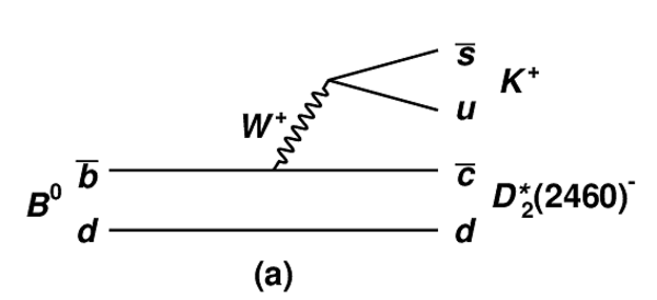
Feynman diagrams for the contributions to $ B ^0 \rightarrow D K ^+ \pi ^- $ from (a) $ B ^0 \rightarrow D_2^*(2460)^- K ^+ $, (b) $ B ^0 \rightarrow \overline{ D }{} {}^0 K ^* (892)^0$ and (c) $ B ^0 \rightarrow D ^0 K ^* (892)^0$ decays.

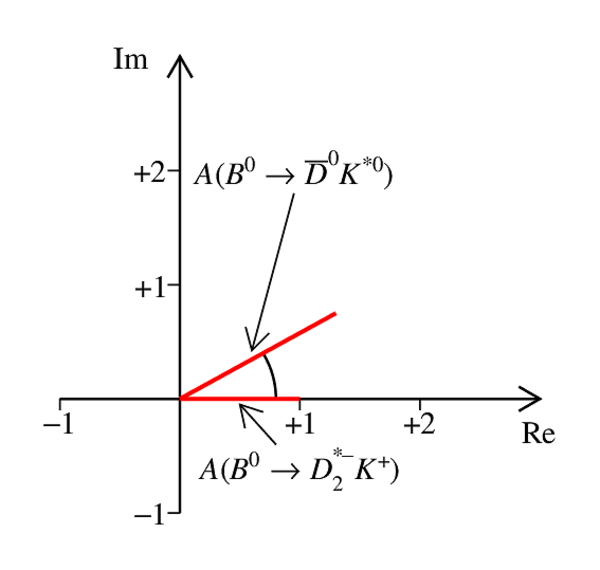
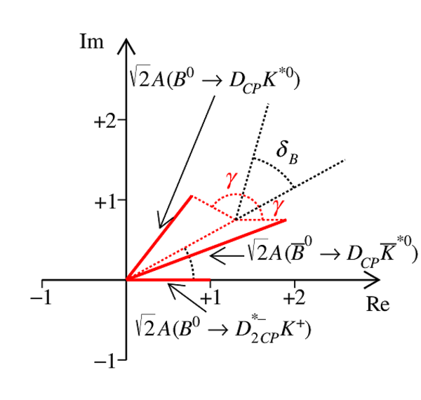
Illustration of the method to determine $\gamma$ from Dalitz plot analysis of $ B ^0 \rightarrow D K ^+ \pi ^- $ decays [12,13]: (left) the $V_{cb}$ amplitude for $ B ^0 \rightarrow \overline{ D }{} {}^0 K ^{*0} $ compared to that for $ B ^0 \rightarrow D_2^{*-} K ^+ $ decay; (right) the effect of the $V_{ub}$ amplitude that contributes to $ B ^0 \rightarrow D_{ C P } K ^{*0} $ and $\overline{ B }{} {}^0 \rightarrow D_{ C P }\overline{ K }{} {}^{*0} $ decays provides sensitivity to $\gamma$. The notation $D_{ C P }$ represents a neutral $ D $ meson reconstructed in a $ C P$ eigenstate, while $D^{*-}_{2 C P }$ denotes the decay chain $D_2^{*-}\rightarrow D _{ C P }\pi ^- $, where the charge of the pion tags the flavour of the neutral $ D $ meson, independently of the mode in which it is reconstructed, so there is no contribution from the $V_{ub}$ amplitude.

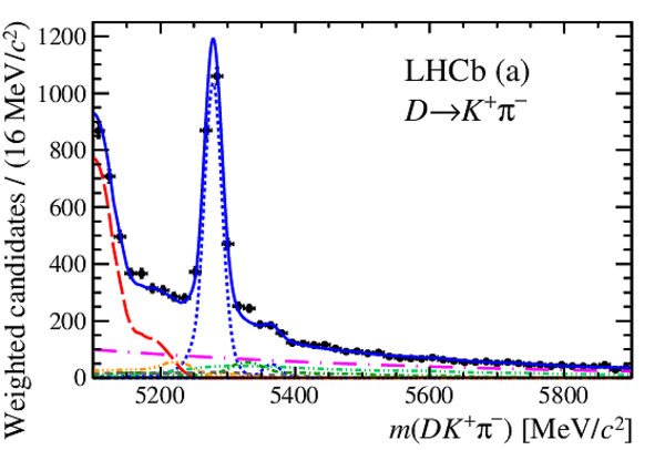
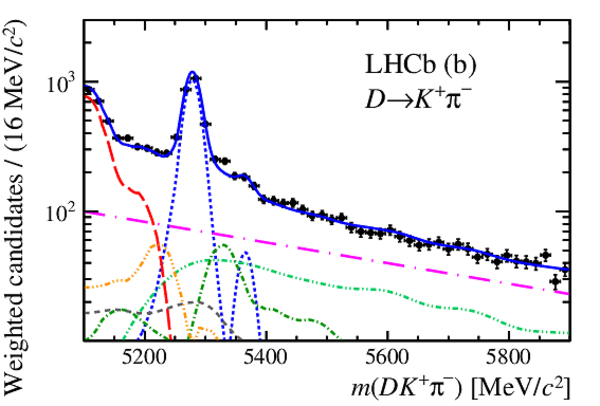
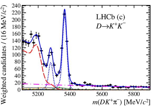
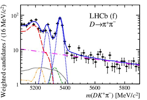
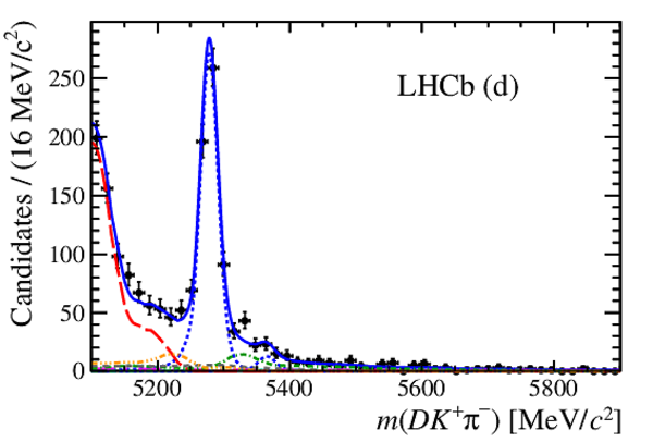
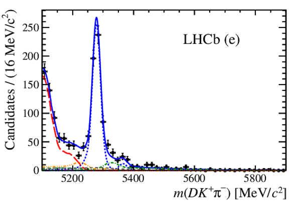
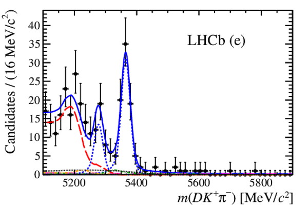
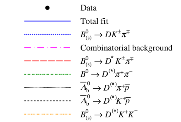
Results of fits to $D K ^+ \pi ^- $ candidates in the (a,b) $D\rightarrow K ^+ \pi ^- $, (c,d) $D\rightarrow K ^+ K ^- $ and (e,f) $D\rightarrow \pi ^+ \pi ^- $ samples. The data and the fit results in each NN output bin have been weighted according to ${\cal S}/({\cal S}+{\cal B})$ as described in the text. The left and right plots are identical but with (left) linear and (right) logarithmic $y$-axis scales. The components are as described in the legend.

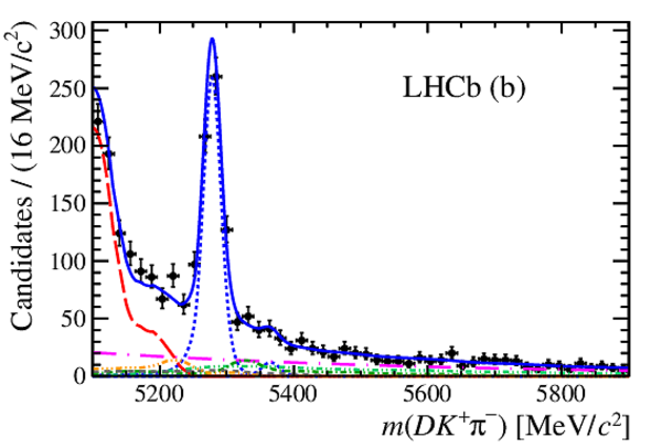
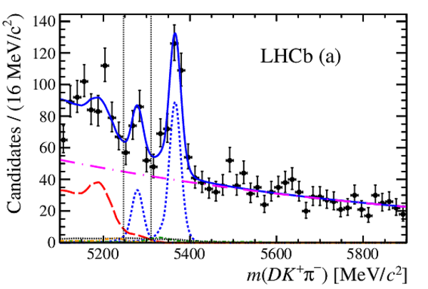
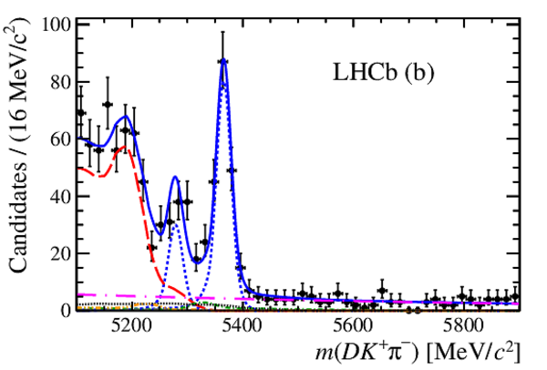
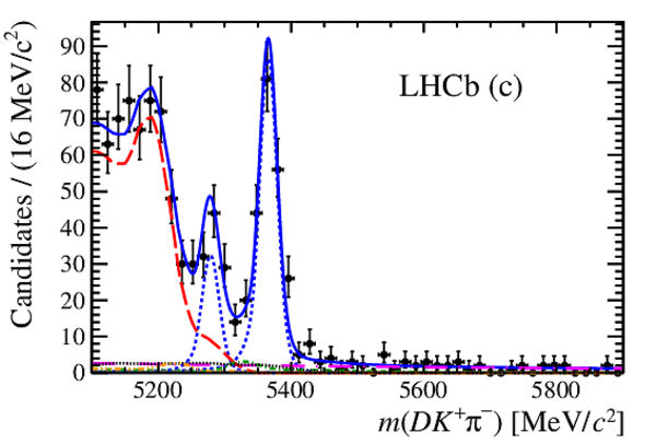
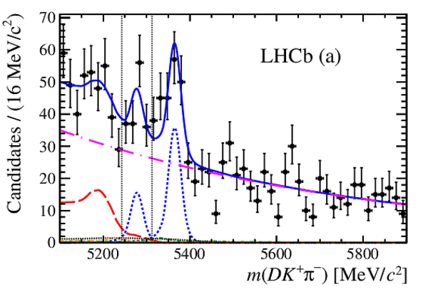
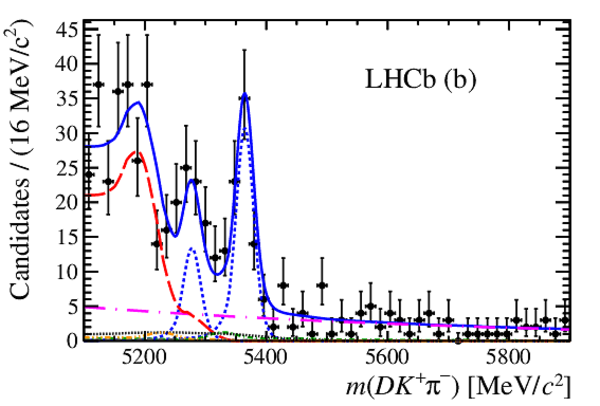
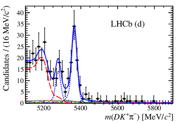
Results of the fit to $ D K ^+ \pi ^- $, $ D \rightarrow K ^+ \pi ^- $ candidates shown separately in the five bins of the neural network output variable. The bins are shown, from (a)--(e), in order of increasing ${\cal S}/{\cal B}$. The components are as indicated in the legend. The vertical dotted lines in (a) show the signal window used for the fit to the Dalitz plot.

Results of the fit to $ D K ^+ \pi ^- $, $ D \rightarrow K ^+ K ^- $ candidates shown separately in the five bins of the neural network output variable. The bins are shown, from (a)--(e), in order of increasing ${\cal S}/{\cal B}$. The components are as indicated in the legend. The vertical dotted lines in (a) show the signal window used for the fit to the Dalitz plot.

Results of the fit to $ D K ^+ \pi ^- $, $ D \rightarrow \pi ^+ \pi ^- $ candidates shown separately in the five bins of the neural network output variable. The bins are shown, from (a)--(e), in order of increasing ${\cal S}/{\cal B}$. The components are as indicated in the legend. The vertical dotted lines in (a) show the signal window used for the fit to the Dalitz plot.

Dalitz plots for candidates in the $ B $ candidate mass signal region in the $ D \rightarrow K ^+ K ^- $ and $\pi ^+ \pi ^- $ samples for (a) $\overline{ B }{} {}^0$ and (b) $ B ^0$ candidates. Only candidates in the three purest NN bins are included. Background has not been subtracted, and therefore some contribution from $\overline{ B }{} {}^0_ s \rightarrow D ^{*0} K ^+ \pi ^- $ decays is expected at low $m(D K ^+ )$ ( i.e. along the top right diagonal).

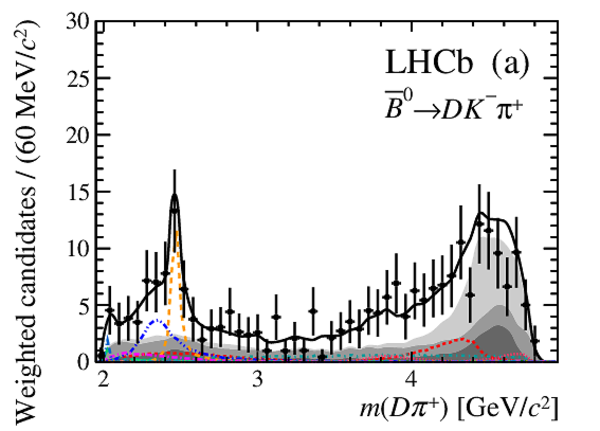
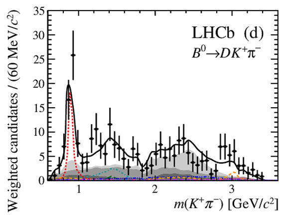
Projections of the $D\rightarrow K ^+ K ^- $ and $\pi ^+ \pi ^- $ samples and the fit result onto (a,b) $m( D \pi ^\mp )$, (c,d) $m( K ^\pm \pi ^\mp )$ and (e,f) $m( D K ^\pm )$ for (a,c,e) $\overline{ B }{} {}^0$ and (b,d,f) $ B ^0$ candidates. The data and the fit results in each NN output bin have been weighted according to ${\cal S}/({\cal S}+{\cal B})$ and combined. The components are described in the legend.

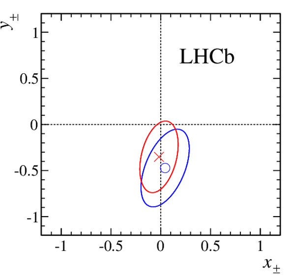
Contours at $68 \%$ CL for the (blue) $(x_+,y_+)$ and (red) $(x_-,y_-)$ parameters associated with the $ B ^0 \rightarrow D K ^* (892)^0$ decay, with statistical uncertainties only. The central values are marked by a circle and a cross, respectively.

Results of likelihood scans for (a) $\gamma$, (b) $r_B$ and (c) $\delta_B$.

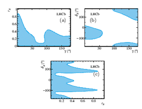
Confidence level contours for (a) $\gamma$ and $r_B$, (b) $\gamma$ and $\delta_B$ and (c) $r_B$ and $\delta_B$. The shaded regions are allowed at $68 \%$ CL.

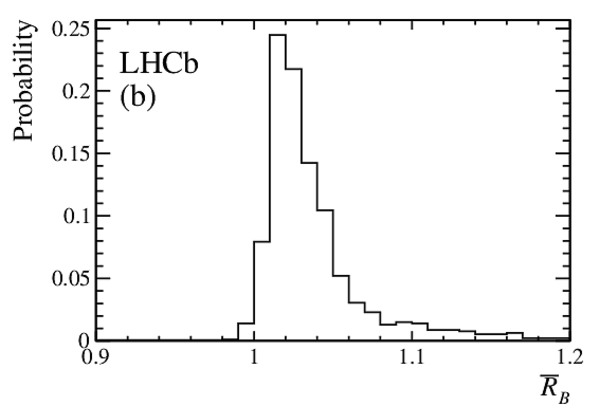
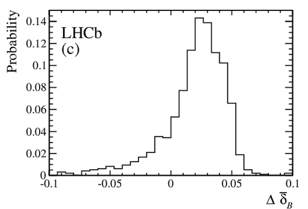
Distributions of (a) $\kappa$, (b) $\bar{R}_B$ and (c) $\Delta \bar{\delta}_B$, obtained as described in the text.

Animated gif made out of all figures.

Yields in the signal window of the fit components in the five NN output bins for the $ D \rightarrow K ^+ \pi ^- $ sample. The last column indicates whether or not each component is explicitly modelled in the Dalitz plot fit.

Yields in the signal window of the fit components in the five NN output bins for the $ D \rightarrow K ^+ K ^- $ sample. The last column indicates whether or not each component is explicitly modelled in the Dalitz plot fit.

Yields in the signal window of the fit components in the five NN output bins for the $ D \rightarrow \pi ^+ \pi ^- $ sample. The last column indicates whether or not each component is explicitly modelled in the Dalitz plot fit.

Results for the unconstrained parameters obtained from the fits to the three data samples. Entries where no number is given are fixed to zero. Fractions marked * are not varied in the fit, and give the difference between unity and the sum of the other fractions.

Experimental systematic uncertainties.

Model uncertainties.

Results for the complex coefficients $c_j$ from the fit to data. Uncertainties are statistical only. All reported quantities are unconstrained in the fit, except that the $D^{*}_{2}(2460)^{-}$ component is fixed as a reference amplitude, and the magnitude of the $D^{*}_{s1}(2700)^{+}$ component is constrained. The $ K ^+ \pi ^- $ S-wave is the coherent sum of the $ K ^*_0 (1430)^{0}$ and the nonresonant $K\pi$ S-wave component [52].

Correlation matrices associated to the (left) statistical and (right) systematic uncertainties of the $ C P$ violation parameters associated with the $ B ^0 \rightarrow D K ^* (892)^0$ decay.