Measurement of the CKM angle $\gamma$ from a combination of LHCb results
[to restricted-access page]Information
LHCb-PAPER-2016-032
CERN-EP-2016-270
arXiv:1611.03076 [PDF]
(Submitted on 09 Nov 2016)
JHEP 12 (2016) 087
Inspire 1496635
Tools
Abstract
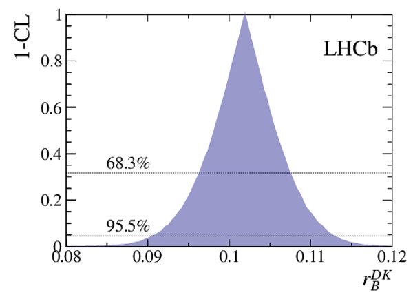
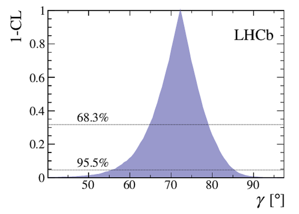
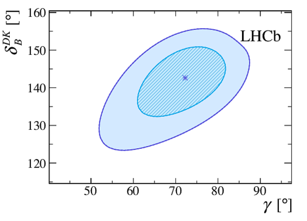
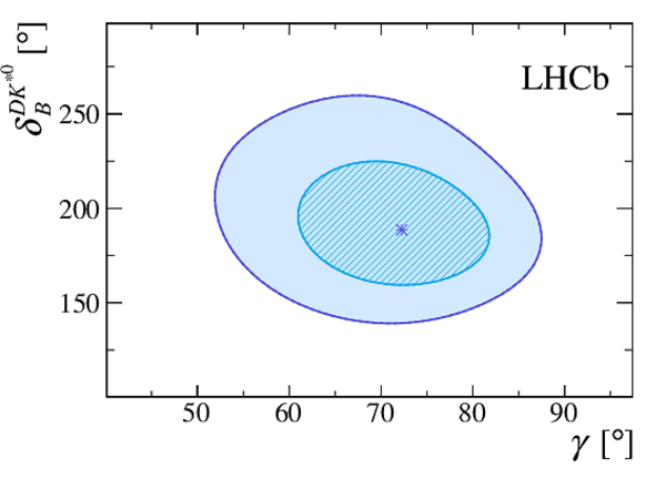
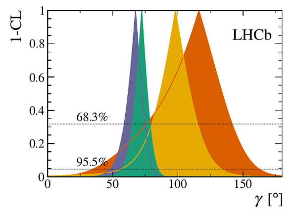
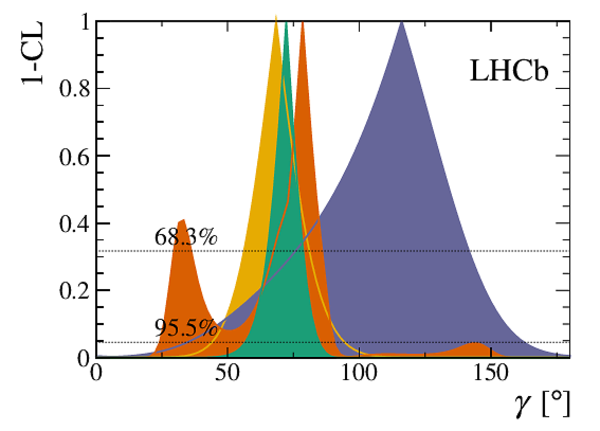
A combination of measurements sensitive to the CKM angle $\gamma$ from LHCb is performed. The inputs are from analyses of time-integrated $B^{+}\rightarrow DK^+$, $B^{0} \rightarrow D K^{*0}$, $B^{0} \rightarrow D K^+ \pi^-$ and $B^{+} \rightarrow D K^+\pi^+\pi^-$ tree-level decays. In addition, results from a time-dependent analysis of $B_{s}^{0} \rightarrow D_{s}^{\mp}K^{\pm}$ decays are included. The combination yields $\gamma = (72.2^{+6.8}_{-7.3})^\circ$, where the uncertainty includes systematic effects. The 95.5 confidence level interval is determined to be $\gamma \in [55.9,85.2]^\circ$. A second combination is investigated, also including measurements from $B^{+} \rightarrow D \pi^+$ and $B^{+} \rightarrow D \pi^+\pi^-\pi^+$ decays, which yields compatible results.
Figures and captions


![HiDef png [157 KiB]](Directory_LHCb-PAPER-2016-032/hidef_Fig1a.png)
![HiDef png [159 KiB]](Directory_LHCb-PAPER-2016-032/hidef_Fig1b.png)
![HiDef png [152 KiB]](Directory_LHCb-PAPER-2016-032/hidef_Fig1c.png)
![HiDef png [153 KiB]](Directory_LHCb-PAPER-2016-032/hidef_Fig1d.png)
![HiDef png [152 KiB]](Directory_LHCb-PAPER-2016-032/hidef_Fig1e.png)
![HiDef png [317 KiB]](Directory_LHCb-PAPER-2016-032/hidef_Fig2a.png)
![HiDef png [344 KiB]](Directory_LHCb-PAPER-2016-032/hidef_Fig2b.png)
![HiDef png [355 KiB]](Directory_LHCb-PAPER-2016-032/hidef_Fig2c.png)
![HiDef png [328 KiB]](Directory_LHCb-PAPER-2016-032/hidef_Fig2d.png)
![HiDef png [317 KiB]](Directory_LHCb-PAPER-2016-032/hidef_Fig2e.png)
![HiDef png [317 KiB]](Directory_LHCb-PAPER-2016-032/hidef_Fig2f.png)
![HiDef png [155 KiB]](Directory_LHCb-PAPER-2016-032/hidef_Fig3a.png)
![HiDef png [158 KiB]](Directory_LHCb-PAPER-2016-032/hidef_Fig3b.png)
![HiDef png [151 KiB]](Directory_LHCb-PAPER-2016-032/hidef_Fig3c.png)
![HiDef png [154 KiB]](Directory_LHCb-PAPER-2016-032/hidef_Fig3d.png)
![HiDef png [174 KiB]](Directory_LHCb-PAPER-2016-032/hidef_Fig3e.png)
![HiDef png [162 KiB]](Directory_LHCb-PAPER-2016-032/hidef_Fig3f.png)
![HiDef png [150 KiB]](Directory_LHCb-PAPER-2016-032/hidef_Fig3g.png)
![HiDef png [244 KiB]](Directory_LHCb-PAPER-2016-032/hidef_Fig4a.png)
![HiDef png [257 KiB]](Directory_LHCb-PAPER-2016-032/hidef_Fig4b.png)
![HiDef png [301 KiB]](Directory_LHCb-PAPER-2016-032/hidef_Fig4c.png)
![HiDef png [254 KiB]](Directory_LHCb-PAPER-2016-032/hidef_Fig4d.png)
![HiDef png [245 KiB]](Directory_LHCb-PAPER-2016-032/hidef_Fig4e.png)
![HiDef png [309 KiB]](Directory_LHCb-PAPER-2016-032/hidef_Fig4f.png)
![HiDef png [276 KiB]](Directory_LHCb-PAPER-2016-032/hidef_Fig4g.png)
![HiDef png [314 KiB]](Directory_LHCb-PAPER-2016-032/hidef_Fig4h.png)
![HiDef png [259 KiB]](Directory_LHCb-PAPER-2016-032/hidef_Fig4i.png)
![HiDef png [115 KiB]](Directory_LHCb-PAPER-2016-032/hidef_Fig5a.png)
![HiDef png [127 KiB]](Directory_LHCb-PAPER-2016-032/hidef_Fig5b.png)
![HiDef png [302 KiB]](Directory_LHCb-PAPER-2016-032/hidef_Fig6a.png)
![HiDef png [324 KiB]](Directory_LHCb-PAPER-2016-032/hidef_Fig6b.png)
![HiDef png [107 KiB]](Directory_LHCb-PAPER-2016-032/hidef_Fig6c.png)
![HiDef png [92 KiB]](Directory_LHCb-PAPER-2016-032/hidef_Fig6d.png)
![HiDef png [452 KiB]](Directory_LHCb-PAPER-2016-032/hidef_Fig7a.png)
![HiDef png [396 KiB]](Directory_LHCb-PAPER-2016-032/hidef_Fig7b.png)
![HiDef png [128 KiB]](Directory_LHCb-PAPER-2016-032/hidef_Fig7c.png)
![HiDef png [459 KiB]](Directory_LHCb-PAPER-2016-032/hidef_Fig8a.png)
![HiDef png [411 KiB]](Directory_LHCb-PAPER-2016-032/hidef_Fig8b.png)
![HiDef png [107 KiB]](Directory_LHCb-PAPER-2016-032/hidef_Fig8c.png)
![HiDef png [172 KiB]](Directory_LHCb-PAPER-2016-032/hidef_Fig9a.png)
![HiDef png [185 KiB]](Directory_LHCb-PAPER-2016-032/hidef_Fig9b.png)
![HiDef png [172 KiB]](Directory_LHCb-PAPER-2016-032/hidef_Fig9c.png)
![HiDef png [169 KiB]](Directory_LHCb-PAPER-2016-032/hidef_Fig9d.png)
![HiDef png [176 KiB]](Directory_LHCb-PAPER-2016-032/hidef_Fig9e.png)
![HiDef png [345 KiB]](Directory_LHCb-PAPER-2016-032/hidef_Fig10a.png)
![HiDef png [375 KiB]](Directory_LHCb-PAPER-2016-032/hidef_Fig10b.png)
![HiDef png [340 KiB]](Directory_LHCb-PAPER-2016-032/hidef_Fig10c.png)
![HiDef png [379 KiB]](Directory_LHCb-PAPER-2016-032/hidef_Fig10d.png)
![HiDef png [376 KiB]](Directory_LHCb-PAPER-2016-032/hidef_Fig10e.png)
![HiDef png [380 KiB]](Directory_LHCb-PAPER-2016-032/hidef_Fig10f.png)
![HiDef png [172 KiB]](Directory_LHCb-PAPER-2016-032/hidef_Fig11a.png)
![HiDef png [189 KiB]](Directory_LHCb-PAPER-2016-032/hidef_Fig11b.png)
![HiDef png [170 KiB]](Directory_LHCb-PAPER-2016-032/hidef_Fig11c.png)
![HiDef png [171 KiB]](Directory_LHCb-PAPER-2016-032/hidef_Fig11d.png)
![HiDef png [237 KiB]](Directory_LHCb-PAPER-2016-032/hidef_Fig11e.png)
![HiDef png [195 KiB]](Directory_LHCb-PAPER-2016-032/hidef_Fig11f.png)
![HiDef png [173 KiB]](Directory_LHCb-PAPER-2016-032/hidef_Fig11g.png)
![HiDef png [347 KiB]](Directory_LHCb-PAPER-2016-032/hidef_Fig12a.png)
![HiDef png [395 KiB]](Directory_LHCb-PAPER-2016-032/hidef_Fig12b.png)
![HiDef png [397 KiB]](Directory_LHCb-PAPER-2016-032/hidef_Fig12c.png)
![HiDef png [386 KiB]](Directory_LHCb-PAPER-2016-032/hidef_Fig12d.png)
![HiDef png [384 KiB]](Directory_LHCb-PAPER-2016-032/hidef_Fig12e.png)
![HiDef png [372 KiB]](Directory_LHCb-PAPER-2016-032/hidef_Fig12f.png)
![HiDef png [262 KiB]](Directory_LHCb-PAPER-2016-032/hidef_Fig12g.png)
![HiDef png [460 KiB]](Directory_LHCb-PAPER-2016-032/hidef_Fig12h.png)
![HiDef png [257 KiB]](Directory_LHCb-PAPER-2016-032/hidef_Fig12i.png)
Tables and captions
|
List of the LHCb measurements used in the combinations. |
Table_1.pdf [63 KiB] HiDef png [88 KiB] Thumbnail [40 KiB] tex code |

|
|
List of the auxiliary inputs used in the combinations. |
Table_2.pdf [81 KiB] HiDef png [102 KiB] Thumbnail [48 KiB] tex code |

|
|
Confidence intervals and central values for the parameters of interest in the frequentist $ DK$ combination. |
Table_3.pdf [52 KiB] HiDef png [60 KiB] Thumbnail [26 KiB] tex code |

|
|
Confidence intervals and central values for the parameters of interest in the frequentist $ Dh$ combination. |
Table_4.pdf [52 KiB] HiDef png [80 KiB] Thumbnail [35 KiB] tex code |

|
|
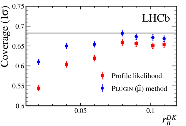
Measured coverage $\alpha$ of the confidence intervals for $\gamma$ , determined at the best fit points, for both the one-dimensional {\sc Plugin} and profile likelihood methods. The nominal coverage is denoted as $\eta$. |
Table_5.pdf [38 KiB] HiDef png [58 KiB] Thumbnail [30 KiB] tex code |

|
|
Credible intervals and most probable values for the hadronic parameters determined from the $ DK$ Bayesian combination. |
Table_6.pdf [52 KiB] HiDef png [61 KiB] Thumbnail [27 KiB] tex code |

|
|
Credible intervals and most probable values for the hadronic parameters determined from the $ Dh$ Bayesian combination. |
Table_7.pdf [52 KiB] HiDef png [85 KiB] Thumbnail [39 KiB] tex code |

|
|
$ D ^0$ decay time acceptance coefficients (see Ref. [37]) for each analysis. |
Table_8.pdf [58 KiB] HiDef png [103 KiB] Thumbnail [46 KiB] tex code |

|
|
Correlation matrix of the statistical uncertainties for the $ B ^+ \rightarrow D h^+$ , $ D ^0 \rightarrow h^+h^-$ observables [44]. |
Table_9.pdf [42 KiB] HiDef png [73 KiB] Thumbnail [28 KiB] tex code |

|
|
Correlation matrix of the systematic uncertainties for the $ B ^+ \rightarrow D h^+$ , $ D ^0 \rightarrow h^+h^-$ observables [44]. |
Table_10.pdf [42 KiB] HiDef png [80 KiB] Thumbnail [31 KiB] tex code |

|
|
Correlation matrix of the statistical uncertainties for the $ B ^+ \rightarrow D h^+$ , $ D ^0 \rightarrow h^\pm\pi^\mp\pi^+\pi^-$ observables [44]. |
Table_11.pdf [41 KiB] HiDef png [61 KiB] Thumbnail [23 KiB] tex code |

|
|
Correlation matrix of the systematic uncertainties for the $ B ^+ \rightarrow D h^+$ , $ D ^0 \rightarrow h^\pm\pi^\mp\pi^+\pi^-$ observables [44]. |
Table_12.pdf [41 KiB] HiDef png [57 KiB] Thumbnail [23 KiB] tex code |

|
|
Correlation matrix of the statistical uncertainties for the $ B ^+ \rightarrow D h^+$ , $ D ^0 \rightarrow h^\pm h^\mp \pi ^0 $ observables [52]. |
Table_13.pdf [48 KiB] HiDef png [48 KiB] Thumbnail [19 KiB] tex code |

|
|
Correlation matrix of the systematic uncertainties for the $ B ^+ \rightarrow D h^+$ , $ D ^0 \rightarrow h^\pm h^\mp \pi ^0 $ observables [52]. |
Table_14.pdf [49 KiB] HiDef png [62 KiB] Thumbnail [24 KiB] tex code |

|
|
Correlation matrix of the statistical uncertainties for the $ B ^+ \rightarrow D K ^+ $ , $ D ^0 \rightarrow K ^0_{\mathrm{ \scriptscriptstyle S}} h^+h^-$ observables [46]. |
Table_15.pdf [45 KiB] HiDef png [55 KiB] Thumbnail [25 KiB] tex code |

|
|
Correlation matrix of the systematic uncertainties for the $ B ^+ \rightarrow D K ^+ $ , $ D ^0 \rightarrow K ^0_{\mathrm{ \scriptscriptstyle S}} h^+h^-$ observables [46]. |
Table_16.pdf [45 KiB] HiDef png [56 KiB] Thumbnail [25 KiB] tex code |

|
|
Correlation matrix of the statistical uncertainties for the $ B ^0 \rightarrow D K^{*0}$ , $ D\rightarrow K^+\pi^-$ observables [49]. |
Table_17.pdf [60 KiB] HiDef png [34 KiB] Thumbnail [15 KiB] tex code |

|
|
Correlation matrix of the systematic uncertainties for the $ B ^0 \rightarrow D K^{*0}$ , $ D\rightarrow K^+\pi^-$ observables [49]. |
Table_18.pdf [53 KiB] HiDef png [35 KiB] Thumbnail [15 KiB] tex code |

|
|
Correlation matrix of the statistical uncertainties for $ B ^0 \rightarrow D ^0 K\pi$ , $ D\rightarrow h^+h^-$ observables [50]. |
Table_19.pdf [52 KiB] HiDef png [54 KiB] Thumbnail [25 KiB] tex code |

|
|
Correlation matrix of the systematic uncertainties for $ B ^0 \rightarrow D ^0 K\pi$ , $ D\rightarrow h^+h^-$ observables [50]. |
Table_20.pdf [53 KiB] HiDef png [58 KiB] Thumbnail [26 KiB] tex code |

|
|
Correlation matrix of the statistical uncertainties for the $ B ^0 \rightarrow D K^{*0}$ , $ D\rightarrow K ^0_{\mathrm{ \scriptscriptstyle S}} \pi^+\pi^-$ observables [51]. |
Table_21.pdf [52 KiB] HiDef png [42 KiB] Thumbnail [20 KiB] tex code |

|
|
Correlation matrix of the statistical uncertainties for the $ B ^0_ s \rightarrow D_s^\mp K^\pm$ observables [52]. |
Table_22.pdf [39 KiB] HiDef png [58 KiB] Thumbnail [26 KiB] tex code |

|
|
Correlation matrix of the systematic uncertainties for the $ B ^0_ s \rightarrow D_s^\mp K^\pm$ observables [52]. |
Table_23.pdf [38 KiB] HiDef png [55 KiB] Thumbnail [27 KiB] tex code |

|
|
Correlations of the HFAG charm parameters (CHARM 2015, "Fit 3", $ C P$ violation allowed) [22]. |
Table_24.pdf [40 KiB] HiDef png [63 KiB] Thumbnail [30 KiB] tex code |

|
|
Correlations of the $ D ^0 \rightarrow K^\pm\pi^\mp\pi^+\pi^-$ and $ D ^0 \rightarrow K^\pm\pi^\mp \pi ^0 $ parameters from CLEO and LHCb [58]. |
Table_25.pdf [39 KiB] HiDef png [63 KiB] Thumbnail [33 KiB] tex code |

|
|
Fit parameter correlations for the $ DK$ combination. The fit results are given in Table 3 |
Table_28.pdf [41 KiB] HiDef png [69 KiB] Thumbnail [32 KiB] tex code |

|
|
Fit parameter correlations for the $ Dh$ combination solution 1. The fit results are given in Table 4 |
Table_28.pdf [41 KiB] HiDef png [69 KiB] Thumbnail [32 KiB] tex code |
|
|
Fit parameter correlations for the $ Dh$ combination solution 2. The fit results are given in Table 4 |
Table_28.pdf [41 KiB] HiDef png [69 KiB] Thumbnail [32 KiB] tex code |
|
![HiDef png [88 KiB]](Directory_LHCb-PAPER-2016-032/hidef_Table_1.png)
![HiDef png [102 KiB]](Directory_LHCb-PAPER-2016-032/hidef_Table_2.png)
![HiDef png [60 KiB]](Directory_LHCb-PAPER-2016-032/hidef_Table_3.png)
![HiDef png [80 KiB]](Directory_LHCb-PAPER-2016-032/hidef_Table_4.png)
![HiDef png [58 KiB]](Directory_LHCb-PAPER-2016-032/hidef_Table_5.png)
![HiDef png [61 KiB]](Directory_LHCb-PAPER-2016-032/hidef_Table_6.png)
![HiDef png [85 KiB]](Directory_LHCb-PAPER-2016-032/hidef_Table_7.png)
![HiDef png [103 KiB]](Directory_LHCb-PAPER-2016-032/hidef_Table_8.png)
![HiDef png [73 KiB]](Directory_LHCb-PAPER-2016-032/hidef_Table_9.png)
![HiDef png [80 KiB]](Directory_LHCb-PAPER-2016-032/hidef_Table_10.png)
![HiDef png [61 KiB]](Directory_LHCb-PAPER-2016-032/hidef_Table_11.png)
![HiDef png [57 KiB]](Directory_LHCb-PAPER-2016-032/hidef_Table_12.png)
![HiDef png [48 KiB]](Directory_LHCb-PAPER-2016-032/hidef_Table_13.png)
![HiDef png [62 KiB]](Directory_LHCb-PAPER-2016-032/hidef_Table_14.png)
![HiDef png [55 KiB]](Directory_LHCb-PAPER-2016-032/hidef_Table_15.png)
![HiDef png [56 KiB]](Directory_LHCb-PAPER-2016-032/hidef_Table_16.png)
![HiDef png [34 KiB]](Directory_LHCb-PAPER-2016-032/hidef_Table_17.png)
![HiDef png [35 KiB]](Directory_LHCb-PAPER-2016-032/hidef_Table_18.png)
![HiDef png [54 KiB]](Directory_LHCb-PAPER-2016-032/hidef_Table_19.png)
![HiDef png [58 KiB]](Directory_LHCb-PAPER-2016-032/hidef_Table_20.png)
![HiDef png [42 KiB]](Directory_LHCb-PAPER-2016-032/hidef_Table_21.png)
![HiDef png [58 KiB]](Directory_LHCb-PAPER-2016-032/hidef_Table_22.png)
![HiDef png [55 KiB]](Directory_LHCb-PAPER-2016-032/hidef_Table_23.png)
![HiDef png [63 KiB]](Directory_LHCb-PAPER-2016-032/hidef_Table_24.png)
![HiDef png [63 KiB]](Directory_LHCb-PAPER-2016-032/hidef_Table_25.png)
![HiDef png [69 KiB]](Directory_LHCb-PAPER-2016-032/hidef_Table_28.png)
Created on 02 May 2024.