Expected spectrum of the $\Lambda ^+_ c $ ground state and its orbital excitations from a study based on the nonrelativistic heavy quark - light diquark model [21], along with the observed resonances corresponding to those states [23].

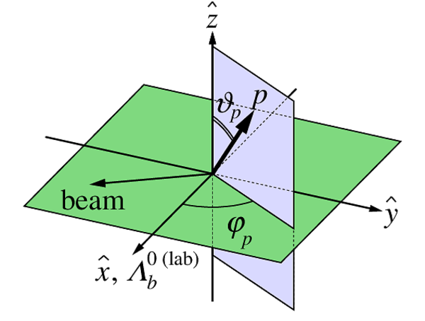
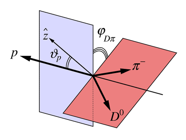
Definition of the angles describing the orientation of the $\Lambda ^0_ b \rightarrow D ^0 p \pi ^- $ decay in the reference frame where the $\Lambda ^0_ b $ baryon is at rest: (a) $\vartheta_p$ and $\varphi_p$, and (b) $\varphi_{D\pi}$.

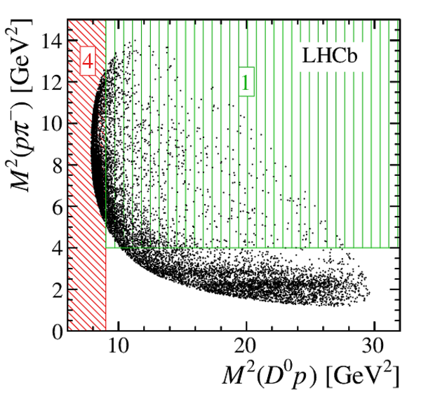
Distributions of $\Lambda ^0_ b \rightarrow D ^0 p \pi ^- $ candidates in data: (a) the full Dalitz plot as a function of $M^2(D^0p)$ and $M^2(p\pi^-)$, and (b) the part of the phase space including the resonances in the $D^0p$ channel (note the change in variable on the horizontal axis). The distributions are neither background-subtracted nor efficiency-corrected. The hatched areas 1--4 are described in the text.

Invariant mass distribution for the $ D ^0 p \pi ^- $ candidates in the entire $ D ^0 p \pi ^- $ phase space. The blue solid line is the fit result. Signal, partially reconstructed and combinatorial background components are shown with different line styles. Vertical lines indicate the boundaries of the signal region used in the amplitude fit.

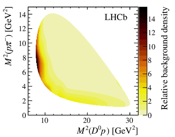
(a) Relative selection efficiency and (b) background density over the $\Lambda ^0_ b \rightarrow D ^0 p \pi ^- $ phase space. The normalisations are such that the average over the phase space is unity.

Fit results for the $\Lambda ^0_ b \rightarrow D ^0 p \pi ^- $ amplitude in the nonresonant region (region 1) (a) $M( D ^0 p )$ projection and (b) $M( p \pi ^- )$ projection. The points with error bars are data, the black histogram is the fit result, and coloured curves show the components of the fit model taking into account the efficiency. The dash-dotted line represents the background. Due to interference effects the total is not necessarily equal to the sum of the components.

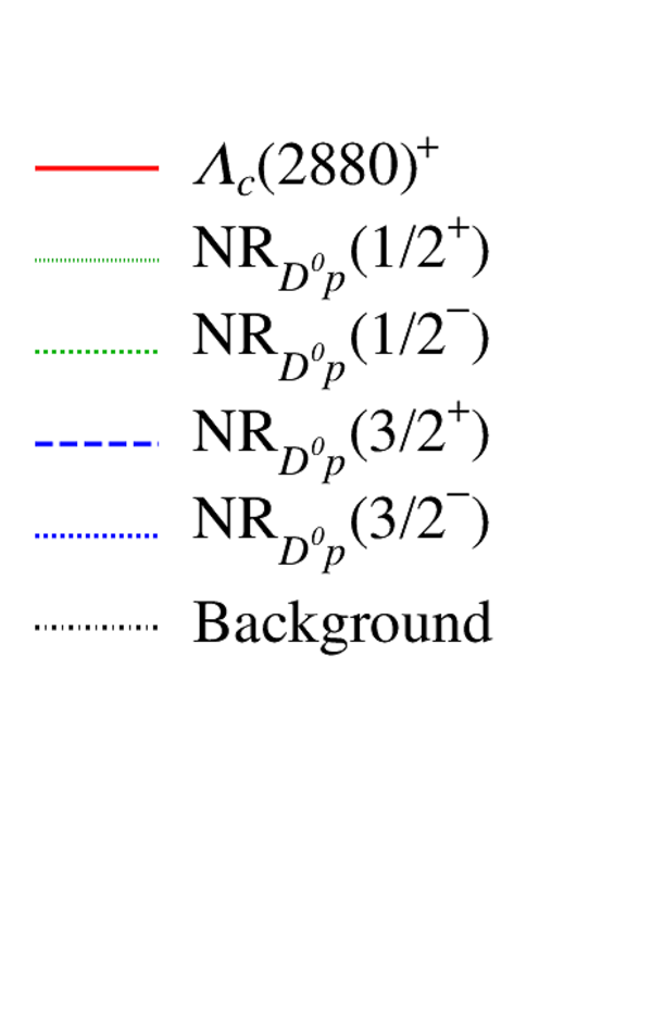
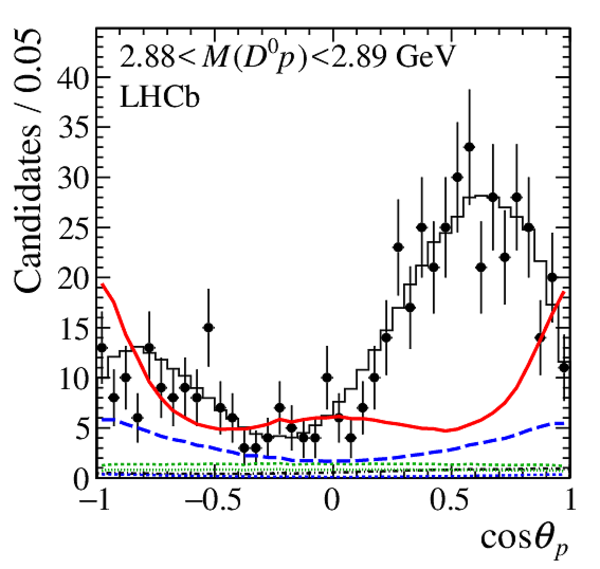
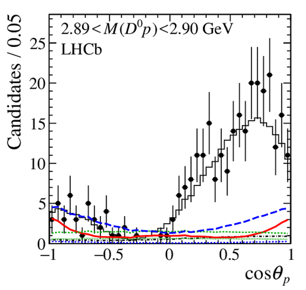
Results of the $\Lambda ^0_ b \rightarrow D ^0 p \pi ^- $ amplitude fit in the $\Lambda _{ c }(2880)^+ $ mass region with spin-parity assignment $J^P=5/2^+$ for the $\Lambda _{ c }(2880)^+$ resonance: (a) $M( D ^0 p )$ projection and (b--e) $\cos\theta_{ p }$ projections in slices of the $ D ^0 p $ invariant mass. The linear nonresonant model is used. Points with error bars are data, the black histogram is the fit result, coloured curves show the components of the fit model. The dash-dotted line represents the background. Vertical lines in (a) indicate the boundaries of the $ D ^0 p $ invariant mass slices. Due to interference effects the total is not necessarily equal to the sum of the components.

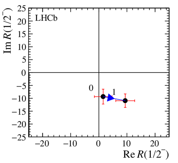
Argand diagrams for the four amplitude components underneath the $\Lambda _{ c }(2880)^+ $ peak in the linear nonresonant model. In each diagram, point 0 corresponds to $M( D ^0 p )=2.86$ $\mathrm{ Ge V}$ , and point 1 to $M( D ^0 p )=2.90$ $\mathrm{ Ge V}$ .

$M( D ^0 p )$ projections for the fit including the $\Lambda _{ c }(2880)^+$ state and four exponential nonresonant amplitudes.

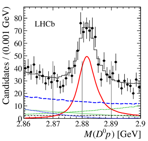
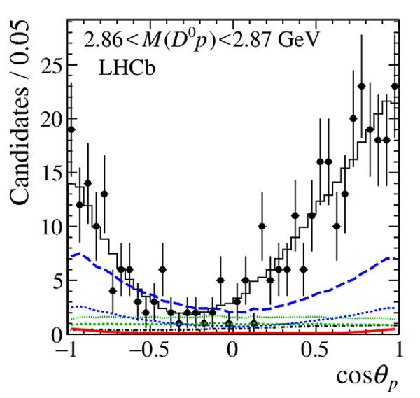
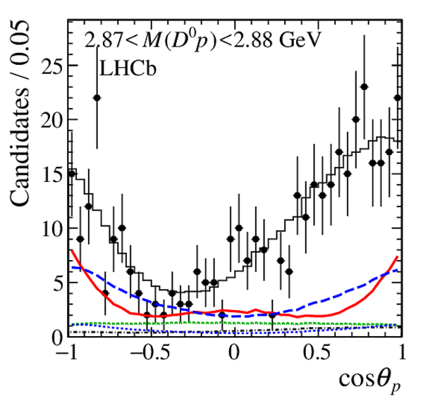
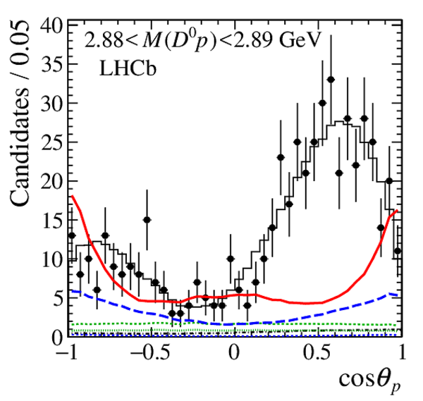
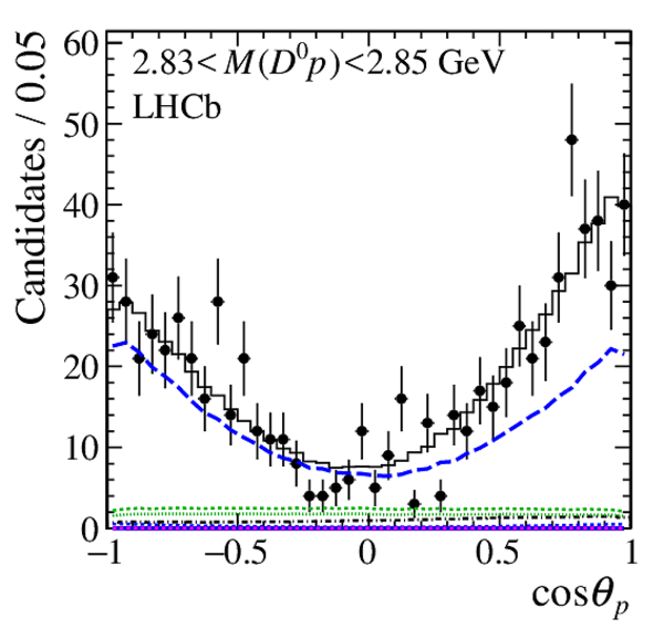
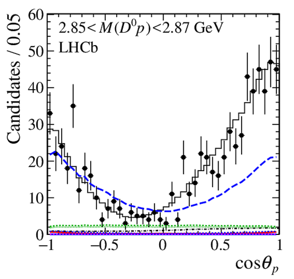
Results for the fit of the $\Lambda ^0_ b \rightarrow D ^0 p \pi ^- $ Dalitz plot distribution in the near-threshold $ D ^0 p $ mass region (region 3): (a) $M( D ^0 p )$ projection, and (b--g) $\cos\theta_{ p }$ projections for slices in $ D ^0 p $ invariant mass. An exponential model is used for the nonresonant partial waves. A broad $\Lambda _{ c }(2860)^+ $ resonance and the $\Lambda _{ c }(2880)^+$ state are also present. Vertical lines in (a) indicate the boundaries of the $ D ^0 p $ invariant mass slices. Due to interference effects the total is not necessarily equal to the sum of the components.

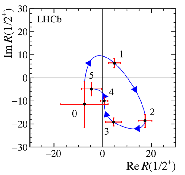
Argand diagrams for the complex spline components used in two fits, represented by blue lines with arrows indicating the phase motion with increasing $M( D ^0 p )$. For subfigure (a), the $J^P=3/2^+$ partial wave is modelled as a spline and the other components in the fit ($1/2^{+}$, $1/2^-$ and $3/2^-$) are described with exponential amplitudes. For comparison, results from a separate fit in which the $3/2^+$ partial wave is described with a Breit--Wigner function are superimposed: the green line represents its phase motion, and the green dots correspond to the $ D ^0 p $ masses at the spline knots. For subfigure (b), the $J^P=1/2^+$ component is modelled as a spline and $1/2^{-}$, $3/2^+$ and $3/2^-$ components as exponential amplitudes.

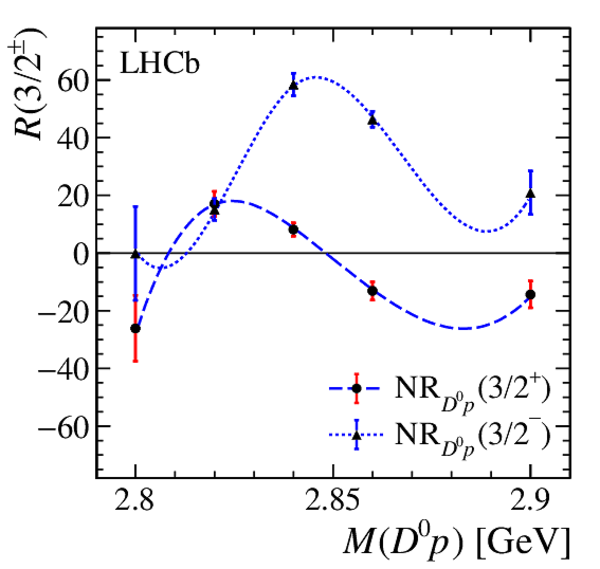
Results of the fit including the $\Lambda _{ c }(2880)^+$ state, two exponential nonresonant amplitudes with $J^P=1/2^{\pm}$ and two real splines in $J^P=3/2^{\pm}$ partial waves. (a) Spline amplitudes for $J^P=3/2^{\pm}$ partial waves as functions of $M( D ^0 p )$. Points with the error bars are fitted values of the amplitude in the spline knots, smooth curves are the interpolated amplitude shapes. (b) The $M( D ^0 p )$ projection of the decay density and the components of the fit model.

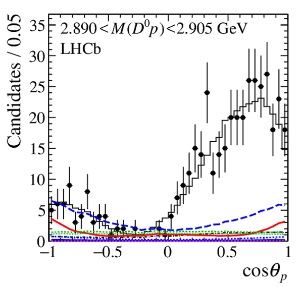
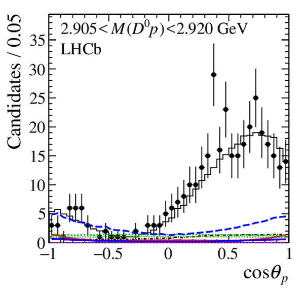
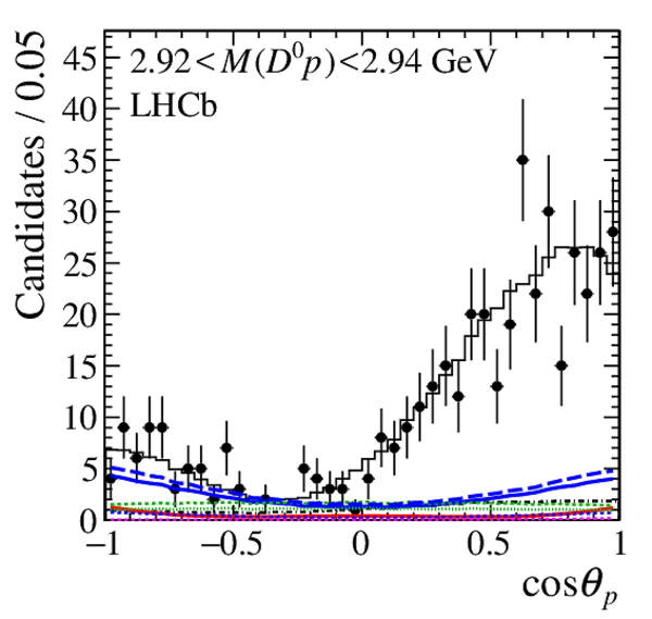
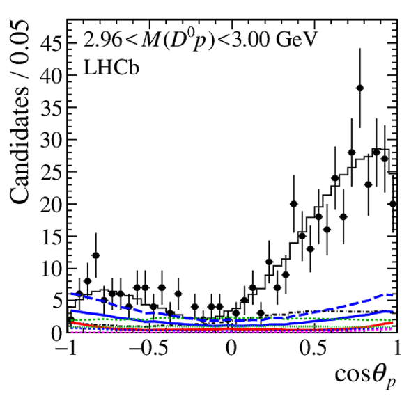
Results of the fit of the $\Lambda ^0_ b \rightarrow D ^0 p \pi ^- $ data in the $ D ^0 p $ mass region including the $\Lambda _{ c }(2880)^+ $ and $\Lambda _{ c }(2940)^+ $ resonances (region 4): (a) $m( D ^0 p )$ projection and (b--k) $\cos\theta_{ p }$ projections for slices of $ D ^0 p $ invariant mass. An exponential model is used for the nonresonant partial waves, and the $J^P=3/2^-$ hypothesis is used for the $\Lambda _{ c }(2940)^+$ state. Vertical lines in (a) indicate the boundaries of the $ D ^0 p $ invariant mass slices. Due to interference effects the total is not necessarily equal to the sum of the components.

Animated gif made out of all figures.

Results of the fits to the $\Lambda ^0_ b \rightarrow D ^0 p \pi ^- $ mass distribution in the entire $\Lambda ^0_ b \rightarrow D ^0 p \pi ^- $ phase space and in the four phase space regions used in the amplitude fits. The signal and background yields for the full $M( D ^0 p \pi ^- )$ range, as well as for the amplitude fit region $|M( D ^0 p \pi ^- )-m(\Lambda ^0_ b )|<30\mathrm{ Me V} $ ("box"), are reported.

Estimated contributions from the $ p \pi ^- $ nonresonant components in different phase space regions. The signal yields from Table 1 are also included for comparison.

Values of the $\Delta\ln\mathcal{L}$ and fit quality for various $\Lambda _{ c }(2880)^+$ spin assignments and nonresonant amplitude models. The baseline model is shown in bold face.

Systematic and model uncertainties on the $\Lambda _{ c }(2880)^+$ parameters and on the value of $\Delta\ln\mathcal{L}$ between the $5/2$ and $7/2$ spin assignments. The uncertainty due to the nonresonant model includes a component associated with the helicity formalism, which for comparison is given explicitly in the table, too.

Quality of various fits to the near-threshold $ D ^0 p $ data. The models include nonresonant components for partial waves with $J\leq 3/2$ with or without a resonant component, whose mass is fixed to 2765 $\mathrm{ Me V}$ or allowed to vary ("Float"). "Exp" denotes an exponential nonresonant lineshape, "CSpl" a complex spline parametrisation, and "RSpl" a real spline parametrisation multiplied by a constant phase. The baseline model is shown in bold face.

Systematic uncertainties on the $\Lambda _{ c }(2860)^+$ parameters and on $\Delta\ln\mathcal{L}$ between the baseline $3/2^+$ and alternative spin-parity assignments. The uncertainty due to the nonresonant model includes a component associated with the helicity formalism, which for comparison is given explicitly in the table, too.

Correlation matrix associated to the statistical uncertainties of the fit results in the fit region 4.

Fit quality for various $\Lambda _{ c }(2940)^+$ spin-parity assignments. Exponential and polynomial parametrisations of the nonresonant lineshapes are considered. The baseline model is shown in bold face.

Systematic and model uncertainties of the $\Lambda _{ c }(2940)^+$ parameters and the resonance fit fractions. The uncertainty due to the nonresonant model includes a component associated with the helicity formalism, which for comparison is given explicitly in the table, too.

Systematic and model uncertainties on $\Delta\ln\mathcal{L}$ between the baseline fit with $J^P=3/2^-$ for the $\Lambda _{ c }(2940)^+$ state and other fits without a $\Lambda _{ c }(2940)^+$ contribution or with other spin-parity assignments, for the exponential nonresonant model.

Systematic and model uncertainties on $\Delta\ln\mathcal{L}$ between the baseline fit with $J^P=3/2^-$ for the $\Lambda _{ c }(2940)^+$ state and other fits without a $\Lambda _{ c }(2940)^+$ contribution or with other spin-parity assignments, for the polynomial nonresonant model.

Significances of the $J^P=3/2^-$ spin-parity assignment for $\Lambda _{ c }(2940)^+$ state with respect to the alternative models without a $\Lambda _{ c }(2940)^+$ contribution or with other spin-parity assignments.