Resonances and $CP$ violation in $B_s^0$ and $\overline{B}_s^0 \to J/\psi K^+K^-$ decays in the mass region above the $\phi(1020)$

Information

LHCb-PAPER-2017-008
CERN-EP-2017-062
arXiv:1704.08217 [PDF]

(Submitted on 26 Apr 2017)
JHEP 08 (2017) 037
Inspire 1596902

Tools

Abstract

The decays of $B_s^0$ and $\overline{B}_s^0$ mesons into the $J/\psi K^+K^-$ final state are studied in the $K^+K^-$ mass region above the $\phi(1020)$ meson in order to determine the resonant substructure and measure the $CP$-violating phase, $\phi_s$, the decay width, $\Gamma_s$, and the width difference between light and heavy mass eigenstates, $\Delta\Gamma_s$. A decay-time dependent amplitude analysis is employed. The data sample corresponds to an integrated luminosity of $3{\rm fb}^{-1}$ produced in 7 and 8 Tev $pp$ collisions at the LHC, collected by the LHCb experiment. The measurement determines $\phi_s = 119\pm107\pm34 {\rm mrad}$. A combination with previous LHCb measurements using similar decays into the $J/\psi \pi^+\pi^-$ and $J/\psi\phi(1020)$ final states gives $\phi_s=1\pm37 {\rm mrad}$, consistent with the Standard Model prediction.

Figures and captions

Definition of the helicity angles.	Fig1new.pdf [8 KiB] HiDef png [28 KiB] Thumbnail [15 KiB]
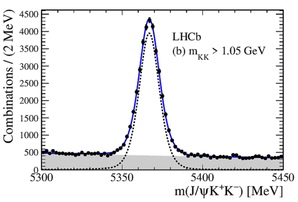
Fits to invariant mass distributions of $ { J \mskip -3mu/\mskip -2mu\psi \mskip 2mu} K^+K^-$ combinations after subtraction of the two reflection backgrounds for (a) $m_{KK}<1.05$ $\mathrm{ Ge V}$ and (b) $m_{KK}>1.05$ $\mathrm{ Ge V}$ . Total fits are shown by solid (blue) lines, the signal by dashed (black) lines, and the combinatorial background by darkened regions. Note that the combinatorial background in (a) is too small to be easily visible.	Fig2a.pdf [22 KiB] HiDef png [171 KiB] Thumbnail [157 KiB]
	Fig2b.pdf [22 KiB] HiDef png [208 KiB] Thumbnail [203 KiB]
Invariant mass squared of $K^+K^-$ versus $ { J \mskip -3mu/\mskip -2mu\psi \mskip 2mu} K^+$ for $ B ^0_ s \rightarrow { J \mskip -3mu/\mskip -2mu\psi \mskip 2mu} K^+K^-$ candidates within $\pm15$ $\mathrm{ Me V}$ of the $ B ^0_ s $ mass peak. The high intensity $\phi(1020)$ resonance band is shown with a line (light green).	Fig3.pdf [159 KiB] HiDef png [1 MiB] Thumbnail [589 KiB]
Scaled decay-time efficiency $\varepsilon_{\rm data}^{ B ^0_ s }(t)$ in arbitrary units (a.u.) for (a) the $\phi(1020)$ region and (b) the high-mass region.	Fig4a.pdf [17 KiB] HiDef png [146 KiB] Thumbnail [144 KiB]
	Fig4b.pdf [17 KiB] HiDef png [145 KiB] Thumbnail [147 KiB]
Efficiencies projected onto (a) $m_{KK}$, (b) $\cos \theta_{KK}$, (c) $\cos \theta_{ { J \mskip -3mu/\mskip -2mu\psi \mskip 2mu} }$ and (d) $\chi$ in arbitrary units (a.u.), obtained from simulation of $ B ^0_ s \rightarrow { J \mskip -3mu/\mskip -2mu\psi \mskip 2mu} K ^+ K ^- $ phase-space decays (points with error bars), while the curves show the parameterization from the efficiency model.	Fig5a.pdf [17 KiB] HiDef png [130 KiB] Thumbnail [128 KiB]
	Fig5b.pdf [16 KiB] HiDef png [131 KiB] Thumbnail [129 KiB]
	Fig5c.pdf [16 KiB] HiDef png [130 KiB] Thumbnail [128 KiB]
	Fig5d.pdf [16 KiB] HiDef png [121 KiB] Thumbnail [117 KiB]
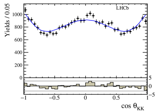
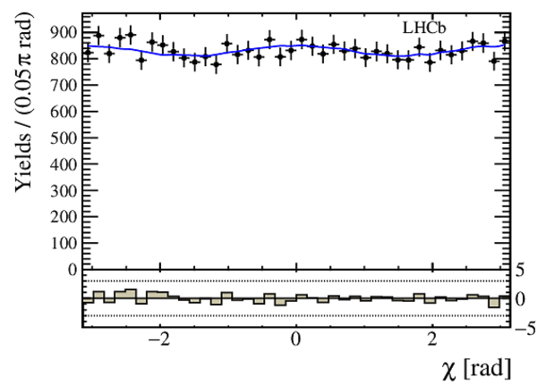
Projections of the fitting variables in the (left) low-mass ($\phi(1020)$) and (right) high-mass regions shown by the solid (blue) curves. The points with error bars are the data. At the bottom of each figure the differences between the data and the fit divided by the uncertainty in the data are shown.	Fig6l1.pdf [23 KiB] HiDef png [202 KiB] Thumbnail [175 KiB]
	Fig6r1.pdf [24 KiB] HiDef png [220 KiB] Thumbnail [189 KiB]
	Fig6l2.pdf [23 KiB] HiDef png [179 KiB] Thumbnail [159 KiB]
	Fig6r2.pdf [23 KiB] HiDef png [167 KiB] Thumbnail [149 KiB]
	Fig6l3.pdf [22 KiB] HiDef png [172 KiB] Thumbnail [153 KiB]
	Fig6r3.pdf [21 KiB] HiDef png [168 KiB] Thumbnail [145 KiB]
	Fig6l4.pdf [22 KiB] HiDef png [170 KiB] Thumbnail [153 KiB]
	Fig6r4.pdf [22 KiB] HiDef png [179 KiB] Thumbnail [168 KiB]
	Fig6l5.pdf [25 KiB] HiDef png [197 KiB] Thumbnail [176 KiB]
	Fig6r5.pdf [26 KiB] HiDef png [206 KiB] Thumbnail [186 KiB]
Fit projection of $m_{KK}$. The points represent the data; the resonances $\phi(1020)$, $f_2^\prime(1525)$, $\phi(1680)$ are shown by magenta, brown, and cyan long-dashed curves, respectively; the S-wave component is depicted by green long-dashed curves; the other $f_2$ resonances are described by black solid curves; and the total fit by a blue solid curve. At the bottom the differences between the data and the fit divided by the uncertainty in the data are shown.	Fig_7_new.pdf [28 KiB] HiDef png [342 KiB] Thumbnail [267 KiB]
The $K^+K^-$ mass dependence of the spherical harmonic moments of $\cos \theta_{KK}$ in the region of the $\phi(1020)$ resonance after efficiency corrections and background subtraction. The points with error bars are the data points and the (blue) lines are derived from the fit model.	SPH_phi0.pdf [12 KiB] HiDef png [148 KiB] Thumbnail [145 KiB]
	SPH_phi2.pdf [13 KiB] HiDef png [132 KiB] Thumbnail [128 KiB]
	SPH_phi4.pdf [14 KiB] HiDef png [146 KiB] Thumbnail [148 KiB]
The $K^+K^-$ mass dependence of the spherical harmonic moments of $\cos \theta_{KK}$ above the $\phi(1020)$ resonance region after efficiency corrections and background subtraction. The points with error bars are the data points and the (blue) lines are derived from the fit model.	SPH0.pdf [12 KiB] HiDef png [144 KiB] Thumbnail [135 KiB]
	SPH2.pdf [13 KiB] HiDef png [147 KiB] Thumbnail [147 KiB]
	SPH4.pdf [14 KiB] HiDef png [160 KiB] Thumbnail [165 KiB]
Animated gif made out of all figures.	PAPER-2017-008.gif Thumbnail

Tables and captions

Breit-Wigner resonance parameters.	Table_1.pdf [62 KiB] HiDef png [80 KiB] Thumbnail [39 KiB] tex code
Fit results for the $ B ^0_ s $ decay observables in the high $m_{KK}$ region.	Table_2.pdf [50 KiB] HiDef png [68 KiB] Thumbnail [32 KiB] tex code
Fit results of the resonant structure.	Table_3.pdf [54 KiB] HiDef png [80 KiB] Thumbnail [38 KiB] tex code
Fitted phase differences between two transversity states (statistical uncertainty only). Here the symbol $\phi$ refers to the components of the $\phi(1020)$ meson.	Table_4.pdf [45 KiB] HiDef png [256 KiB] Thumbnail [120 KiB] tex code
Absolute systematic uncertainties for the physics parameters determined from the high $m_{KK}$ region compared to the corresponding statistical uncertainty. Here $M_0$ and $\Gamma_0$ refer to the uncertainties on the $f_2^\prime(1525)$ resonance mass and width.	Table_5.pdf [74 KiB] HiDef png [84 KiB] Thumbnail [39 KiB] tex code
Combined systematic and statistical uncertainties in the fit fractions using an absolute scale where the numbers are in units of %. "Res. modelling" refers to resonance modelling.	Table_6.pdf [57 KiB] HiDef png [58 KiB] Thumbnail [25 KiB] tex code
The correlation matrix from the high-mass region fit, taking into account both statistical and systematic uncertainties.	Table_7.pdf [32 KiB] HiDef png [43 KiB] Thumbnail [20 KiB] tex code
The correlation matrix taking into account both statistical and systematic uncertainties for the combination of the three measurements $ B ^0_ s \rightarrow { J \mskip -3mu/\mskip -2mu\psi \mskip 2mu} K^+K^-$ for $m_{KK}>1.05$ GeV, $m_{KK}<1.05$ GeV, and $ { J \mskip -3mu/\mskip -2mu\psi \mskip 2mu} \pi^+\pi^-$.	Table_8.pdf [31 KiB] HiDef png [42 KiB] Thumbnail [19 KiB] tex code