Feynman diagrams for $\overline{ B }{} {}^0_ s \rightarrow D_{\hspace{-0.0625em}s} ^+ K^-$ decays (left) without and (right) with $ B ^0_ s $ -- $\overline{ B }{} {}^0_ s $ mixing.

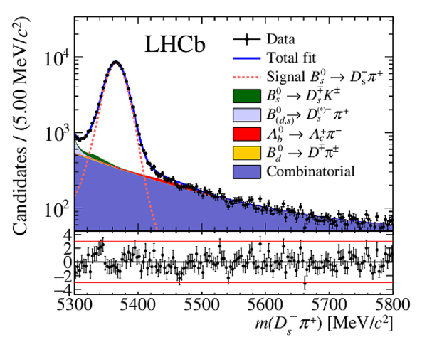
Distributions of the (upper left) $ B ^0_ s $ and (upper right) $ D ^-_ s $ invariant masses for $ B ^0_ s \rightarrow D ^-_ s \pi ^+ $ final states, and (bottom) of the logarithm of the companion track PID log-likelihood, $\ln(L(\pi/K))$. In each plot, the contributions from all $ D ^-_ s $ final states are combined. The solid blue curve is the total result of the simultaneous fit. The dotted red curve shows the $ B ^0_ s \rightarrow D ^-_ s \pi ^+ $ signal and the fully coloured stacked histograms show the different background contributions. Normalised residuals are shown underneath all distributions.

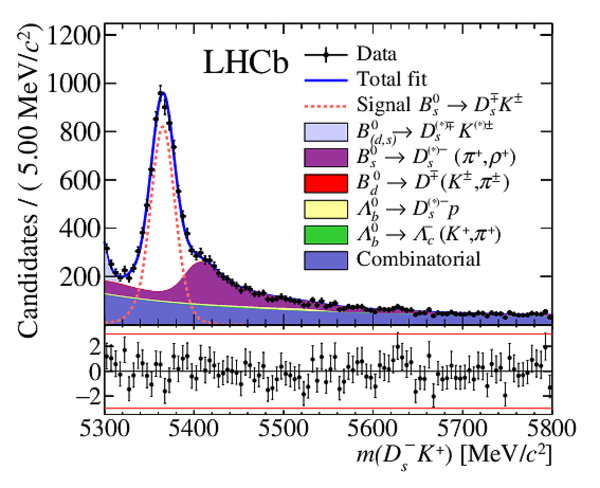
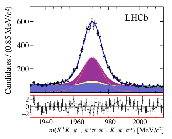
Distributions of the (upper left) $ B ^0_ s $ and (upper right) $ D ^-_ s $ invariant masses for $ B ^0_ s \rightarrow D_{\hspace{-0.0625em}s} ^\mp K^\pm$ final states, and (bottom) of the logarithm of the companion track PID log-likelihood, $\ln(L(K/\pi))$. In each plot, the contributions from all $ D ^-_ s $ final states are combined. The solid blue curve is the total result of the simultaneous fit. The dotted red curve shows the $ B ^0_ s \rightarrow D ^-_ s \pi ^+ $ signal and the fully coloured stacked histograms show the different background contributions. Normalised residuals are shown underneath all distributions.

Data points show the measured resolution $\sigma$ as a function of the per-candidate uncertainty $\sigma_t$ for prompt $D_s^{\mp}$ candidates combined with a random track. The dashed lines indicate the values used to determine the systematic uncertainties on this method. The solid line shows the linear fit to the data as discussed in the text. The histogram overlaid is the distribution of the per-candidate decay-time uncertainty for $ B ^0_ s \rightarrow D_{\hspace{-0.0625em}s} ^\mp K^\pm$ candidates.

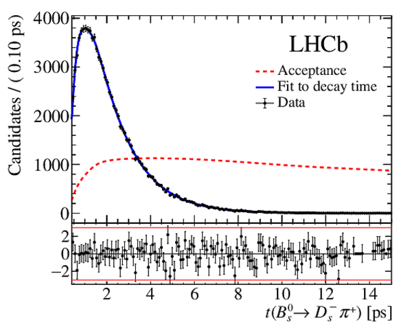
Decay time distribution of $ B ^0_ s \rightarrow D ^-_ s \pi ^+ $ candidates obtained by the sPlot technique. The solid blue curve is the result of the \it sFit procedure and the dashed red curve shows the measured decay-time acceptance in arbitrary units. Normalised residuals are shown underneath.

The (top) decay-time distribution of $ B ^0_ s \rightarrow D_{\hspace{-0.0625em}s} ^\mp K^\pm$ candidates obtained by the sPlot technique. The solid blue curve is the result of the \it sFit procedure and the dashed red curve shows the decay-time acceptance in arbitrary units, obtained from the \it sFit procedure applied to the $ B ^0_ s \rightarrow D ^-_ s \pi ^+ $ candidates and corrected for the ratio of decay-time acceptances of $ B ^0_ s \rightarrow D_{\hspace{-0.0625em}s} ^\mp K^\pm$ and $ B ^0_ s \rightarrow D ^-_ s \pi ^+ $ from simulation. Normalised residuals are shown underneath. The $ C P$ -asymmetry plots for (bottom left) the $ D ^+_ s K^-$ final state and (bottom right) the $ D ^-_ s K^+$ final state, folded into one mixing period $2\pi/\Delta m_s $, are also shown.

Profile likelihood contours of (top left) $ r_{ D_{\hspace{-0.0625em}s} \hspace{-0.0625em} K }$ vs. $\gamma$ , and (top right) $\delta$ vs. $\gamma$ . The markers denote the best-fit values. The contours correspond to 68.3% CL (95.5% CL). The graph on the bottom left shows $ 1-{\rm CL}$ for the angle $\gamma$ , together with the central value and the 68.3% CL interval as obtained from the frequentist method described in the text. The bottom right plot shows a visualisation of how each of the amplitude coefficients contributes towards the overall constraint on the weak phase, $\gamma - 2\beta_s $ . The difference between the phase of $(- {A_{ f }^{\Delta\Gamma}} , S_{ f } )$ and $(- {A_{\overline{ f } }^{\Delta\Gamma}} , S_{\overline{ f } } )$ is proportional to the strong phase $\delta $, which is close to $360^\circ$ and thus not indicated in the figure.

Animated gif made out of all figures.

Calibration parameters and tagging asymmetries of the OS and SS taggers obtained from $ B ^0_ s \rightarrow D ^-_ s \pi ^+ $ decays. The first uncertainty is statistical and the second is systematic.

Performances of the flavour tagging for $ B ^0_ s \rightarrow D ^-_ s \pi ^+ $ candidates tagged by OS only, SS only and both OS and SS algorithms.

Values of the $ C P$ -violation parameters obtained from the fit to the decay-time distribution of $ B ^0_ s \rightarrow D_{\hspace{-0.0625em}s} ^\mp K^\pm$ decays. The first uncertainty is statistical and the second is systematic.

Statistical correlation matrix of the $ C P$ parameters. Other fit parameters have negligible correlations with the $ C P$ parameters.

Systematic uncertainties on the $ C P$ parameters, relative to the statistical uncertainties.

Correlation matrix of the total systematic uncertainties of the $ C P$ parameters.