Evidence for the decay $B_{s}^0 \rightarrow \overline{K}{}^{*0}\mu^+\mu^-$

Information

LHCb-PAPER-2018-004
CERN-EP-2018-059
arXiv:1804.07167 [PDF]

(Submitted on 19 Apr 2018)
JHEP 07 (2018) 020
Inspire 1668916

Tools

Abstract

A search for the decay $B_{s}^0 \rightarrow \overline{K}{}^{*0}\mu^+\mu^-$ is presented using data sets corresponding to 1.0, 2.0 and 1.6 $\text{fb}^{-1}$ of integrated luminosity collected during $pp$ collisions with the LHCb experiment at centre-of-mass energies of 7, 8 and 13 TeV, respectively. An excess is found over the background-only hypothesis with a significance of 3.4 standard deviations. The branching fraction of the $B_{s}^0 \rightarrow \overline{K}{}^{*0}\mu^+\mu^-$ decay is determined to be $\mathcal{B}(B_{s}^0 \rightarrow \overline{K}{}^{*0}\mu^+\mu^-) = [2.9 \pm 1.0 (\text{stat}) \pm 0.2 (\text{syst}) \pm 0.3 (\text{norm})] \times 10^{-8}$, where the first and second uncertainties are statistical and systematic, respectively. The third uncertainty is due to limited knowledge of external parameters used to normalise the branching fraction measurement.

Figures and captions

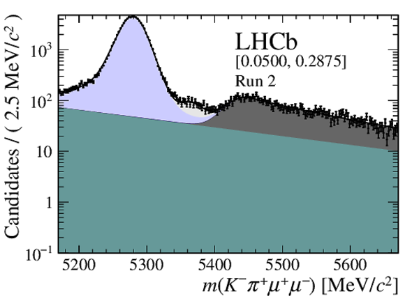
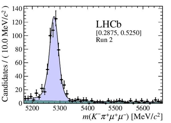
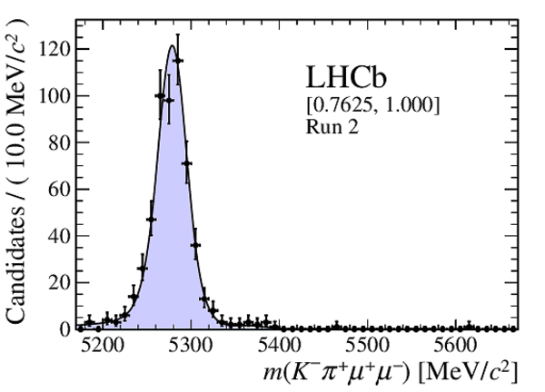
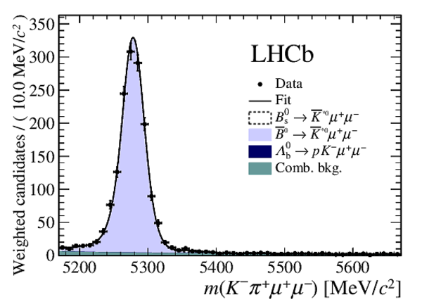
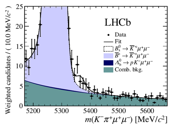
Distribution of reconstructed $ K ^- \pi ^+ \mu ^+\mu ^- $ invariant mass of candidates outside the $ { J \mskip -3mu/\mskip -2mu\psi \mskip 2mu}$ and $\psi {(2S)}$ mass regions, summing the three highest neural network response bins of each run condition. The candidates are shown (left) over the full range and (right) over a restricted vertical range to emphasise the $ B ^0_ s \rightarrow \overline{ K }{} {}^{0} \mu ^+\mu ^- $ component. The solid line indicates a combination of the results of the fits to the individual bins. Components are detailed in the legend, where they are shown in the same order as they are stacked in the figure. The background from misidentified $ B ^0 \rightarrow K ^{0} \mu ^+\mu ^- $ decays is included in the $\overline{ B }{} {}^0 \rightarrow \overline{ K }{} {}^{*0} \mu ^+\mu ^- $ component.	Fig1a.pdf [31 KiB] HiDef png [240 KiB] Thumbnail [215 KiB] *.C file
	Fig1b.pdf [20 KiB] HiDef png [293 KiB] Thumbnail [251 KiB] *.C file
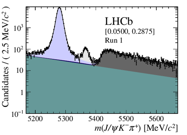
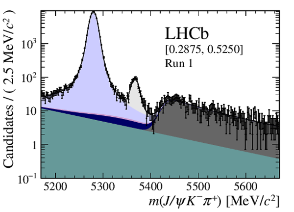
Distribution of reconstructed $ { J \mskip -3mu/\mskip -2mu\psi \mskip 2mu} K ^- \pi ^+ $ invariant mass of the candidates in the $ { J \mskip -3mu/\mskip -2mu\psi \mskip 2mu}$ mass region summing the three highest neural network response bins of each run condition, shown (left) over the full range and (right) over a restricted vertical range to emphasise the $ B ^0_ s \rightarrow { J \mskip -3mu/\mskip -2mu\psi \mskip 2mu} \overline{ K }{} {}^{0} $ component. The solid line indicates a combination of the results of the fits to the individual bins. Components are detailed in the legend, where they are shown in the same order as they are stacked in the figure. The background from misidentified $ B ^0 \rightarrow { J \mskip -3mu/\mskip -2mu\psi \mskip 2mu} K ^{0} $ decays is included in the $\overline{ B }{} {}^0 \rightarrow { J \mskip -3mu/\mskip -2mu\psi \mskip 2mu} \overline{ K }{} {}^{*0} $ component.	Fig2a.pdf [56 KiB] HiDef png [224 KiB] Thumbnail [200 KiB] *.C file
	Fig2b.pdf [58 KiB] HiDef png [328 KiB] Thumbnail [271 KiB] *.C file
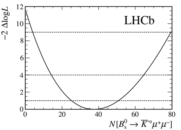
Change in log-likelihood from the simultaneous fit to the candidates in the two data-taking periods and the different bins of neural network response, as a function of the $ B ^0_ s \rightarrow \overline{ K }{} {}^{*0} \mu ^+\mu ^- $ yield. Systematic uncertainties on the yield have been included in the likelihood.	Fig3.pdf [14 KiB] HiDef png [97 KiB] Thumbnail [57 KiB] *.C file
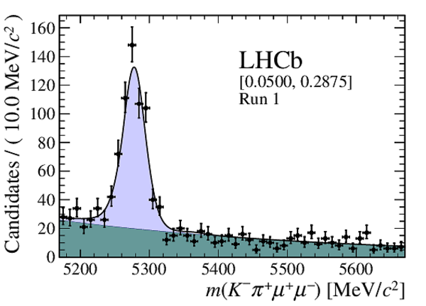
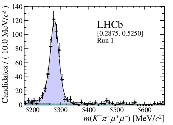
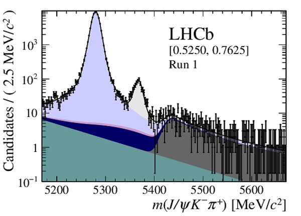
Distribution of reconstructed $ K ^- \pi ^+ \mu ^+\mu ^- $ invariant mass of candidates in the $ { J \mskip -3mu/\mskip -2mu\psi \mskip 2mu}$ mass window in (top four figures) the Run 1 and (bottom four figures) Run 2 data sets. The candidates are divided into four independent bins of increasing neural network response per data taking period.	Fig4a.pdf [63 KiB] HiDef png [261 KiB] Thumbnail [221 KiB] *.C file
	Fig4b.pdf [64 KiB] HiDef png [288 KiB] Thumbnail [249 KiB] *.C file
	Fig4c.pdf [61 KiB] HiDef png [281 KiB] Thumbnail [244 KiB] *.C file
	Fig4d.pdf [56 KiB] HiDef png [271 KiB] Thumbnail [238 KiB] *.C file
	Fig4e.pdf [62 KiB] HiDef png [247 KiB] Thumbnail [213 KiB] *.C file
	Fig4f.pdf [63 KiB] HiDef png [286 KiB] Thumbnail [243 KiB] *.C file
	Fig4g.pdf [62 KiB] HiDef png [310 KiB] Thumbnail [262 KiB] *.C file
	Fig4h.pdf [57 KiB] HiDef png [281 KiB] Thumbnail [242 KiB] *.C file
Distribution of reconstructed $ K ^- \pi ^+ \mu ^+\mu ^- $ invariant mass of candidates outside of the $ { J \mskip -3mu/\mskip -2mu\psi \mskip 2mu}$ and $\psi {(2S)}$ mass regions in (top four figures) the Run 1 and (bottom four figures) Run 2 data sets. The candidates are divided into four independent bins of increasing neural network response per data taking period.	Fig5a.pdf [38 KiB] HiDef png [268 KiB] Thumbnail [227 KiB] *.C file
	Fig5b.pdf [38 KiB] HiDef png [223 KiB] Thumbnail [194 KiB] *.C file
	Fig5c.pdf [38 KiB] HiDef png [200 KiB] Thumbnail [180 KiB] *.C file
	Fig5d.pdf [38 KiB] HiDef png [211 KiB] Thumbnail [184 KiB] *.C file
	Fig5e.pdf [34 KiB] HiDef png [273 KiB] Thumbnail [236 KiB] *.C file
	Fig5f.pdf [38 KiB] HiDef png [238 KiB] Thumbnail [204 KiB] *.C file
	Fig5g.pdf [38 KiB] HiDef png [210 KiB] Thumbnail [190 KiB] *.C file
	Fig5h.pdf [37 KiB] HiDef png [204 KiB] Thumbnail [183 KiB] *.C file
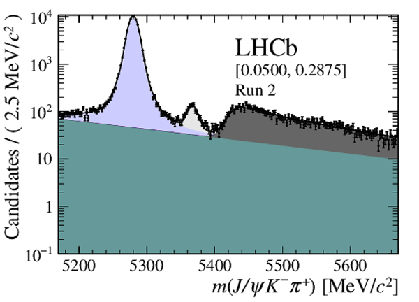
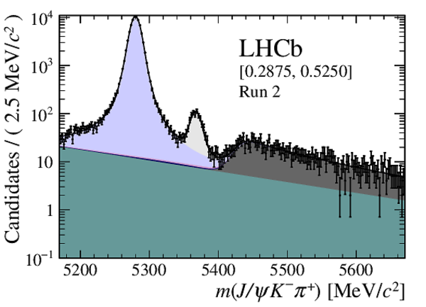
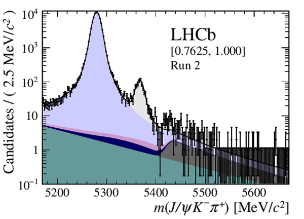
Distribution of reconstructed $ { J \mskip -3mu/\mskip -2mu\psi \mskip 2mu} K ^- \pi ^+ $ invariant mass after application of a $ { J \mskip -3mu/\mskip -2mu\psi \mskip 2mu}$ mass constraint of candidates in (top four figures) the Run 1 and (bottom four figures) Run 2 data sets. The candidates are divided into four independent bins of increasing neural network response per data taking period.	Fig6a.pdf [67 KiB] HiDef png [275 KiB] Thumbnail [229 KiB] *.C file
	Fig6b.pdf [67 KiB] HiDef png [311 KiB] Thumbnail [261 KiB] *.C file
	Fig6c.pdf [68 KiB] HiDef png [334 KiB] Thumbnail [276 KiB] *.C file
	Fig6d.pdf [59 KiB] HiDef png [327 KiB] Thumbnail [267 KiB] *.C file
	Fig6e.pdf [66 KiB] HiDef png [258 KiB] Thumbnail [219 KiB] *.C file
	Fig6f.pdf [66 KiB] HiDef png [302 KiB] Thumbnail [250 KiB] *.C file
	Fig6g.pdf [66 KiB] HiDef png [329 KiB] Thumbnail [270 KiB] *.C file
	Fig6h.pdf [60 KiB] HiDef png [329 KiB] Thumbnail [273 KiB] *.C file
Animated gif made out of all figures.	PAPER-2018-004.gif Thumbnail

Tables and captions

Main sources of systematic uncertainty considered on the branching fraction measurements. The first uncertainty applies to the measurement of $\mathcal{B} ( B ^0_ s \rightarrow \overline{ K }{} {}^{*0} \mu ^+\mu ^- )$, the second to $\mathcal{B} ( B ^0_ s \rightarrow \overline{ K }{} {}^{*0} \mu ^+\mu ^- )/\mathcal{B} (\overline{ B }{} {}^0 \rightarrow \overline{ K }{} {}^{*0} \mu ^+\mu ^- )$ and the third to $\mathcal{B} ( B ^0_ s \rightarrow \overline{ K }{} {}^{*0} \mu ^+\mu ^- )/\mathcal{B} ( B ^0_ s \rightarrow { J \mskip -3mu/\mskip -2mu\psi \mskip 2mu} \overline{ K }{} {}^{*0} )$, respectively. A description of the different contributions can be found in the text. The first three sources of uncertainty affect the measured yield of the signal decay. The total uncertainty is the sum in quadrature of the individual sources. The final row indicates the additional uncertainty arising from the uncertainties on external parameters used in the measurements.

Table_1.pdf [86 KiB]
HiDef png [83 KiB]
Thumbnail [36 KiB]
tex code

Supplementary Material [file]

Supplementary material full pdf	supple[..].pdf [232 KiB]
This ZIP file contains supplementary material for the publication LHCb-PAPER-2018-004. The files are: supplemantary.pdf : An overview of the extra text and figures .pdf, .png, .eps, .C : The additional figures in a variaty of file formats	Fig1a-S.pdf [14 KiB] HiDef png [138 KiB] Thumbnail [126 KiB] *C file
	Fig1b-S.pdf [14 KiB] HiDef png [136 KiB] Thumbnail [125 KiB] *C file
	Fig2a-S.pdf [14 KiB] HiDef png [91 KiB] Thumbnail [54 KiB] *C file
	Fig2b-S.pdf [13 KiB] HiDef png [71 KiB] Thumbnail [42 KiB] *C file
	Fig3a-S.pdf [35 KiB] HiDef png [241 KiB] Thumbnail [217 KiB] *C file
	Fig3b-S.pdf [22 KiB] HiDef png [282 KiB] Thumbnail [240 KiB] *C file