Observation of the decay $B_s^0 \to \overline{D}^0 K^+ K^-$

Information

LHCb-PAPER-2018-014
CERN-EP-2018-157
arXiv:1807.01891 [PDF]

(Submitted on 05 Jul 2018)
Phys. Rev. D98 072006 (2018)
Inspire 1681145

Tools

Abstract

The first observation of the $B_s^0 \to \overline{D}^0 K^+ K^-$ decay is reported, together with the most precise branching fraction measurement of the mode $B^0 \to \overline{D}^0 K^+ K^-$. The results are obtained from an analysis of $pp$ collision data corresponding to an integrated luminosity of $3.0 \textrm{fb}^{-1}$. The data were collected with the LHCb detector at centre-of-mass energies of $7$ and $8$ TeV. The branching fraction of the $B^0 \to \overline{D}^0 K^+ K^-$ decay is measured relative to that of the decay $B^0 \to \overline{D}^0 \pi^+ \pi^-$ to be $$\frac{\mathcal{B}(B^0 \to \overline{D}^0 K^+ K^-)}{\mathcal{B}(B^0 \to \overline{D}^0 \pi^+ \pi^-)} = (6.9 \pm 0.4 \pm 0.3)\%,$$ where the first uncertainty is statistical and the second is systematic. The measured branching fraction of the $B_s^0 \to \overline{D}^0 K^+ K^-$ decay mode relative to that of the corresponding $B^0$ decay is $$\frac{\mathcal{B}(B_s^0 \to \overline{D}^0 K^+ K^-)}{\mathcal{B}(B^0 \to \overline{D}^0 K^+ K^-)} = (93.0 \pm 8.9 \pm 6.9)\%.$$ Using the known branching fraction of ${B^0 \to \overline{D}^0 \pi^+ \pi^-}$, the values of ${{\mathcal B}(B^0 \to \overline{D}^0 K^+ K^- )=(6.1 \pm 0.4 \pm 0.3 \pm 0.3) \times 10^{-5}}$, and ${{\cal B}(B_s^0 \to \overline{D}^0 K^+ K^-)=}$ $(5.7 \pm 0.5 \pm 0.4 \pm 0.5) \times 10^{-5}$ are obtained, where the third uncertainties arise from the branching fraction of the decay modes ${B^0 \to \overline{D}^0 \pi^+ \pi^-}$ and $B^0 \to \overline{D}^0 K^+ K^-$, respectively.

Figures and captions

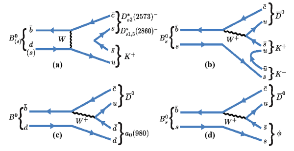
Example Feynman diagrams that contribute to the ${B^0_{(s)} \rightarrow \overline{ D }{} {}^0 K ^+ K ^- }$ decays via (a) $W$-exchange, (b) non-resonant three body mode, (c) and (d) rescattering from a colour-suppressed decay.	Fig1.pdf [263 KiB] HiDef png [332 KiB] Thumbnail [151 KiB] *.C file
Distributions of the Fisher discriminant, for preselected ${ B ^0 \rightarrow \overline{ D }{} {}^0 \pi ^+ \pi ^- }$ data candidates, in the mass range $[5240,5320]$ $ {\mathrm{ Me V /}c^2}$ : (black line) unweighted data distribution, and sWeighted training samples: (blue triangles) signal, (red circles) background, and (green squares) their sum. The training samples are scaled with a factor of two to match the total yield. The cyan (magenta) filled (hatched) histogram displays the simulated ${ B ^0 ( B ^0_ s ) \rightarrow \overline{ D }{} {}^0 K ^+ K ^- }$ decay signal candidates that are normalised to the number of ${ B ^0 \rightarrow \overline{ D }{} {}^0 \pi ^+ \pi ^- }$ normalisation channel candidates (blue triangles). The (magenta) vertical dashed line indicates the position of the nominal selection requirement.	Fig2.pdf [21 KiB] HiDef png [353 KiB] Thumbnail [251 KiB] *.C file
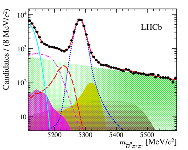
Fit to the ${m_{\overline{ D }{} {}^0 \pi ^+ \pi ^- }}$ invariant-mass distribution with the associated pull plot.	Fig3.pdf [28 KiB] HiDef png [343 KiB] Thumbnail [244 KiB] *.C file
	Fig3a.pdf [13 KiB] HiDef png [53 KiB] Thumbnail [59 KiB] *.C file
Fit to the ${m_{\overline{ D }{} {}^0 K ^+ K ^- }}$ invariant-mass distribution with the associated pull plot.	Fig4.pdf [33 KiB] HiDef png [372 KiB] Thumbnail [268 KiB] *.C file
	Fig4a.pdf [13 KiB] HiDef png [53 KiB] Thumbnail [59 KiB] *.C file
Fit to the (left) ${m_{\overline{ D }{} {}^0 \pi ^+ \pi ^- }}$ invariant mass and (right) ${m_{\overline{ D }{} {}^0 K ^+ K ^- }}$ invariant mass, in logarithmic vertical scale (see the legend on Figs. 3 and 4).	Fig5a.pdf [28 KiB] HiDef png [1 MiB] Thumbnail [462 KiB] *.C file
	Fig5b.pdf [31 KiB] HiDef png [1019 KiB] Thumbnail [420 KiB] *.C file
Dalitz plot for ${ B ^0 \rightarrow \overline{ D }{} {}^0 K ^+ K ^- }$ candidates in the signal region ${m_{\overline{ D }{} {}^0 K ^+ K ^- }\in [5240,5320] {\mathrm{ Me V /}c^2} }$.	Fig6.pdf [19 KiB] HiDef png [241 KiB] Thumbnail [235 KiB] *.C file
Dalitz plot for ${ B ^0_ s \rightarrow \overline{ D }{} {}^0 K ^+ K ^- }$ candidates in the signal region ${m_{\overline{ D }{} {}^0 K ^+ K ^- }\in [5327,5407] {\mathrm{ Me V /}c^2} }$.	Fig7.pdf [16 KiB] HiDef png [166 KiB] Thumbnail [162 KiB] *.C file
Animated gif made out of all figures.	PAPER-2018-014.gif Thumbnail

Tables and captions

Relative yields, in percent, of the various exclusive $b$-hadron decay backgrounds with respect to that of the ${ B ^0 \rightarrow \overline{ D }{} {}^0 \pi ^+ \pi}$ and ${ B ^0_{(s)}\rightarrow \overline{ D }{} {}^0 K ^+ K ^- }$ signal modes. These relative contributions are estimated with simulation in the range $m_{\overline{ D }{} {}^0 h^+ h^-}\in [5115, 6000]$ $ {\mathrm{ Me V /}c^2}$ .	Table_1.pdf [66 KiB] HiDef png [70 KiB] Thumbnail [37 KiB] tex code
Fitted yields that are used as Gaussian constraints in the fit to the ${B^0_{(s)} \rightarrow \overline{ D }{} {}^0 h^+ h^-}$ invariant-mass distributions presented in Sect. 5.2.	Table_2.pdf [63 KiB] HiDef png [36 KiB] Thumbnail [18 KiB] tex code
Parameters from the default fit to ${ B ^0 \rightarrow \overline{ D }{} {}^0 \pi ^+ \pi ^- }$ and ${B^0_{(s)} \rightarrow \overline{ D }{} {}^0 K ^+ K ^- }$ data samples in the invariant-mass range ${m_{\overline{ D }{} {}^0 h^+ h^-}\in[5115, 6000]}$ $ {\mathrm{ Me V /}c^2}$ . The quantity $\chi^2/{\rm ndf}$ corresponds to the reduced $\chi^2$ of the fit for the corresponding number of degrees of freedom, ndf, while the $p$-value is the probability value associated with the fit and is computed with the method of least squares [40].	Table_3.pdf [98 KiB] HiDef png [154 KiB] Thumbnail [75 KiB] tex code
Total efficiencies ${\varepsilon_{B^0_{(s)} \rightarrow \overline{ D }{} {}^0 h^+h^-}}$ and their contributions (before and after accounting for three-body decay kinematic properties) for the each three modes ${ B ^0 \rightarrow \overline{ D }{} {}^0 \pi ^+ \pi ^- }$, ${ B ^0 \rightarrow \overline{ D }{} {}^0 K ^+ K ^- }$, and ${ B ^0_ s \rightarrow \overline{ D }{} {}^0 K ^+ K ^- }$. Uncertainties are statistical only and those smaller than $0.1$ are displayed as $0.1$, but are accounted with their nominal values in the efficiency calculations.	Table_4.pdf [91 KiB] HiDef png [80 KiB] Thumbnail [40 KiB] tex code
Relative systematic uncertainties, in percent, on ${N_{ B ^0 \rightarrow \overline{ D }{} {}^0 \pi ^+ \pi ^- }}$, ${N_{ B ^0 \rightarrow \overline{ D }{} {}^0 K ^+ K ^- }}$ and the ratio ${N_{ B ^0 \rightarrow \overline{ D }{} {}^0 \pi ^+ \pi ^- }}$/${N_{ B ^0 \rightarrow \overline{ D }{} {}^0 K ^+ K ^- }}$ and ${r_{ B ^0_ s / B ^0 }}$, due to PDFs modelling in the $m_{\overline{ D }{} {}^0 \pi ^+ \pi ^- }$ and $m_{\overline{ D }{} {}^0 K ^+ K ^- }$ fits. The uncertainties are uncorrelated and summed in quadrature.	Table_5.pdf [93 KiB] HiDef png [57 KiB] Thumbnail [27 KiB] tex code
Relative systematic uncertainties, in percent, on the ratio of branching fractions $\mathcal{R}_{\overline{ D }{} {}^0 K ^+ K ^- /\overline{ D }{} {}^0 \pi ^+ \pi ^- }$ and $\mathcal{R}_{ B ^0_ s / B ^0 }$. The uncertainties are uncorrelated and summed in quadrature.	Table_6.pdf [75 KiB] HiDef png [45 KiB] Thumbnail [21 KiB] tex code