Measurement of the CKM angle $\gamma$ using $B^\pm\to DK^\pm$ with $D\to K_\text{S}^0\pi^+\pi^-$, $K_\text{S}^0K^+K^-$ decays
[to restricted-access page]Information
LHCb-PAPER-2018-017
CERN-EP-2018-135
arXiv:1806.01202 [PDF]
(Submitted on 04 Jun 2018)
JHEP 08 (2018) 176
Inspire 1676225
Tools
Abstract
A binned Dalitz plot analysis of $B^\pm \to D K^\pm$ decays, with $D\to K_\text{S}^0\pi^+\pi^-$ and $D\to K_\text{S}^0K^+K^-$, is used to perform a measurement of the CP-violating observables $x_{\pm}$ and $y_{\pm}$, which are sensitive to the Cabibbo-Kobayashi-Maskawa angle $\gamma$. The analysis is performed without assuming any $D$ decay model, through the use of information on the strong-phase variation over the Dalitz plot from the CLEO collaboration. Using a sample of proton-proton collision data collected with the LHCb experiment in 2015 and 2016, and corresponding to an integrated luminosity of 2.0$ \text{fb}^{-1}$, the values of the CP violation parameters are found to be $x_- = ( 9.0 \pm 1.7 \pm 0.7 \pm 0.4) \times 10^{-2}$, $y_- = ( 2.1 \pm 2.2 \pm 0.5 \pm 1.1) \times 10^{-2}$, $x_+ = (- 7.7 \pm 1.9 \pm 0.7 \pm 0.4) \times 10^{-2}$, and $y_+ = (- 1.0 \pm 1.9 \pm 0.4 \pm 0.9) \times 10^{-2}$. The first uncertainty is statistical, the second is systematic, and the third is due to the uncertainty on the strong-phase measurements. These values are used to obtain $\gamma = \left(87 ^{+11}_{-12}\right)^\circ$, $r_B = 0.086^{+ 0.013}_{-0.014}$, and $\delta_B = (101 \pm 11)^\circ$, where $r_B$ is the ratio between the suppressed and favoured $B$-decay amplitudes and $\delta_B$ is the corresponding strong-interaction phase difference. This measurement is combined with the result obtained using 2011 and 2012 data collected with the \lhcb experiment, to give $\gamma = \left(80 ^{+10}_{ -9}\right)^\circ$, $r_B = 0.080 \pm 0.011$, and $\delta_B = (110 \pm 10)^\circ$.
Figures and captions
|
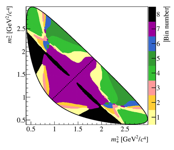
Binning schemes for (left) $ D \rightarrow K ^0_{\mathrm{ \scriptscriptstyle S}} \pi ^+ \pi ^- $ decays and (right) $ D \rightarrow K ^0_{\mathrm{ \scriptscriptstyle S}} K ^+ K ^- $ decays. The diagonal line separates the positive and negative bins, where the positive bins are in the region in which $m^2_->m^2_+$ is satisfied. |
Fig1left.pdf [684 KiB] HiDef png [1 MiB] Thumbnail [446 KiB] *.C file |
|
|
Fig1right.pdf [757 KiB] HiDef png [2 MiB] Thumbnail [486 KiB] *.C file |

|
|
|
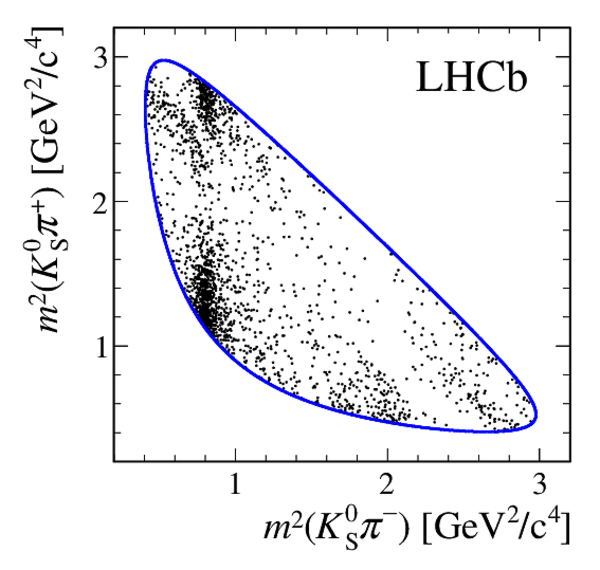
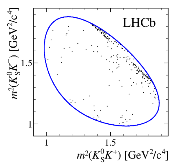
Dalitz plots of long and downstream (left) $ B ^+ \rightarrow D K ^+ $ and (right) $ B ^- \rightarrow D K ^- $ candidates for (top) $ D \rightarrow K ^0_{\mathrm{ \scriptscriptstyle S}} \pi ^+ \pi ^- $ and (bottom) $ D \rightarrow K ^0_{\mathrm{ \scriptscriptstyle S}} K ^+ K ^- $ decays in which the reconstructed invariant mass of the $ B ^\pm$ candidate is in a region of $\pm 25 {\mathrm{ Me V /}c^2} $ around the $ B ^\pm$ mass. The narrow region is chosen to obtain high purity, as no background subtraction has been made. The Dalitz coordinates are calculated using the results of a kinematic fit in which the $ D $ and $ K ^0_{\mathrm{ \scriptscriptstyle S}}$ masses are constrained to their known values. The blue lines show the kinematic boundaries of the decays. |
Fig2to[..].pdf [364 KiB] HiDef png [288 KiB] Thumbnail [270 KiB] *.C file |

|
|
Fig2to[..].pdf [364 KiB] HiDef png [295 KiB] Thumbnail [275 KiB] *.C file |
|
|
|
Fig2bo[..].pdf [178 KiB] HiDef png [180 KiB] Thumbnail [154 KiB] *.C file |
|
|
|
Fig2bo[..].pdf [179 KiB] HiDef png [182 KiB] Thumbnail [159 KiB] *.C file |

|
|
|
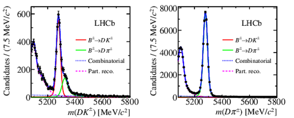
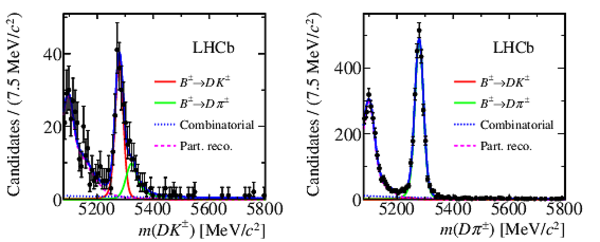
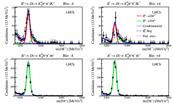
Invariant-mass distributions of (left) $ B ^\pm \rightarrow D K ^\pm $ and (right) $ B ^\pm \rightarrow D \pi ^\pm $ candidates, with $ D \rightarrow K ^0_{\mathrm{ \scriptscriptstyle S}} \pi ^+ \pi ^- $ , shown separately for the (top) long and (bottom) downstream $ K ^0_{\mathrm{ \scriptscriptstyle S}}$ categories. Fit results, including the signal component and background components due to misidentified companions, partially reconstructed decays and combinatorial background, are also shown. |
Fig3top.pdf [37 KiB] HiDef png [237 KiB] Thumbnail [174 KiB] *.C file |

|
|
Fig3bottom.pdf [35 KiB] HiDef png [239 KiB] Thumbnail [176 KiB] *.C file |
|
|
|
Invariant-mass distributions of (left) $ B ^\pm \rightarrow D K ^\pm $ and (right) $ B ^\pm \rightarrow D \pi ^\pm $ candidates, with $ D \rightarrow K ^0_{\mathrm{ \scriptscriptstyle S}} K ^+ K ^- $ , shown separately for the (top) long and (bottom) downstream $ K ^0_{\mathrm{ \scriptscriptstyle S}}$ categories. Fit results, including the signal component and background components due to misidentified companions, partially reconstructed decays and combinatorial background, are also shown. |
Fig4top.pdf [30 KiB] HiDef png [241 KiB] Thumbnail [177 KiB] *.C file |
|
|
Fig4bottom.pdf [35 KiB] HiDef png [236 KiB] Thumbnail [170 KiB] *.C file |

|
|
|
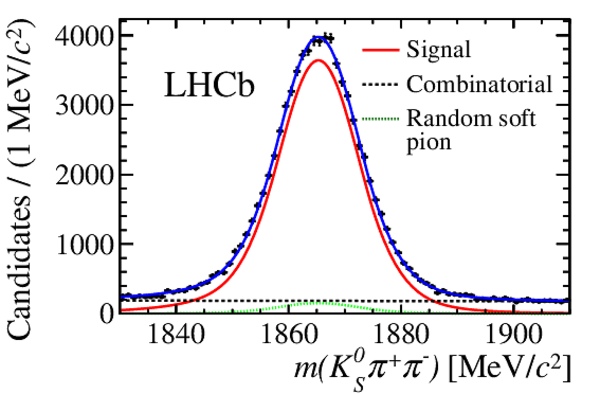
Result of the simultaneous fit to $\optbar{ B}{} \rightarrow D ^{*\pm} \mu^\mp\optbarlowcase{\nu}{} _{ \mu}$ , $ D ^* ^\pm\rightarrow \optbar{ D}{} ^0(\rightarrow K ^0_{\mathrm{ \scriptscriptstyle S}} \pi ^+ \pi ^- )\pi ^\pm $ decays with downstream $ K ^0_{\mathrm{ \scriptscriptstyle S}}$ candidates, in 2016 data. The projections of the fit result are shown for (left) $m( K ^0_{\mathrm{ \scriptscriptstyle S}} \pi ^+ \pi ^- )$ and (right) $\Delta m$. The (blue) total fit PDF is the sum of components describing (solid red) signal, (dashed black) combinatorial background and (dotted green) random soft pion background. |
Fig5a.pdf [24 KiB] HiDef png [271 KiB] Thumbnail [222 KiB] *.C file |
|
|
Fig5b.pdf [30 KiB] HiDef png [221 KiB] Thumbnail [173 KiB] *.C file |

|
|
|
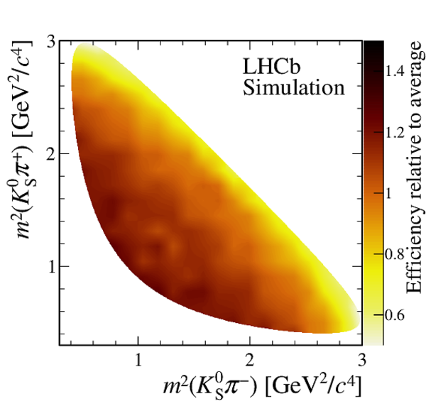
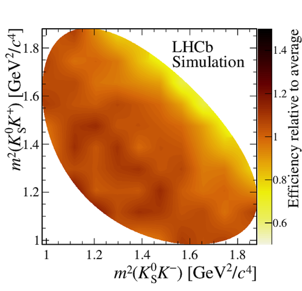
Example efficiency profiles of (left) $ B ^\pm \rightarrow D \pi ^\pm $ and (right) $\optbar{ B}{} \rightarrow D ^{*\pm} \mu^\mp\optbarlowcase{\nu}{} _{ \mu} X$ decays in the simulation. The top (bottom) plots are for $ D \rightarrow K ^0_{\mathrm{ \scriptscriptstyle S}} \pi ^+ \pi ^- $ ( $ D \rightarrow K ^0_{\mathrm{ \scriptscriptstyle S}} K ^+ K ^- $ ) decays. These plots refer to downstream $ K ^0_{\mathrm{ \scriptscriptstyle S}}$ candidates under 2016 data taking conditions. The normalisation is chosen so that the average over the Dalitz plot is unity. |
Fig6a.pdf [480 KiB] HiDef png [1 MiB] Thumbnail [474 KiB] *.C file |

|
|
Fig6b.pdf [475 KiB] HiDef png [1 MiB] Thumbnail [461 KiB] *.C file |
|
|
|
Fig6c.pdf [674 KiB] HiDef png [1 MiB] Thumbnail [522 KiB] *.C file |
|
|
|
Fig6d.pdf [670 KiB] HiDef png [1 MiB] Thumbnail [524 KiB] *.C file |

|
|
|
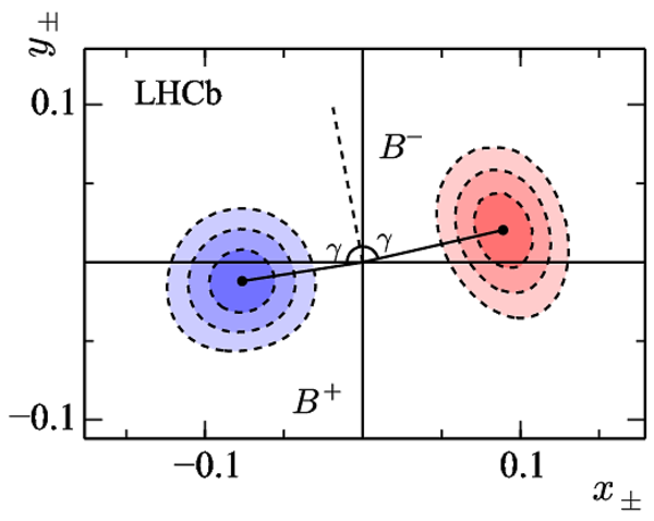
Confidence levels at 68.2%, 95.5% and 99.7% probability for $(x_+,y_+)$ and $(x_{-}, y_{-})$ as measured in $B^\pm \rightarrow D K^\pm$ decays (statistical uncertainties only). The parameters $(x_+,y_+)$ relate to $ B ^+ $ decays and $(x_{-}, y_{-})$ refer to $ B ^- $ decays. The black dots show the central values obtained in the fit. |
Fig7.pdf [30 KiB] HiDef png [194 KiB] Thumbnail [144 KiB] *.C file |
|
|
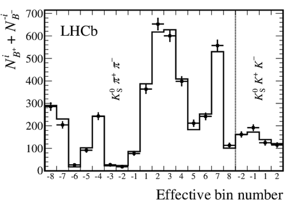
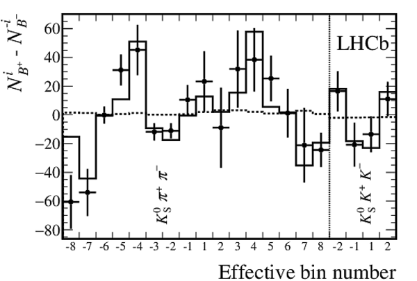
(Left) Comparison of total signal yields from the direct fit (points) to those calculated from the central values of $x_\pm$ and $y_\pm$ (solid line). The yields are given for the effective bin: $+i$ for $ B ^+ $ and $-i$ for $ B ^- $ , and summed over $ B $ charge and $ K ^0_{\mathrm{ \scriptscriptstyle S}} $ decay category. (Right) Comparison of the difference between the $ B ^+ $ and $ B ^- $ yield obtained in the direct fit for each effective bin (points), the prediction from the central values of $x_\pm$ and $y_\pm$ (solid line), and the prediction assuming no $ C P$ violation (dotted line). |
Fig8left.pdf [15 KiB] HiDef png [113 KiB] Thumbnail [66 KiB] *.C file |
|
|
Fig8right.pdf [15 KiB] HiDef png [117 KiB] Thumbnail [73 KiB] *.C file |
|
|
|
Rectangular binning schemes for (left) $ D \rightarrow K ^0_{\mathrm{ \scriptscriptstyle S}} \pi ^+ \pi ^- $ decays and (right) $ D \rightarrow K ^0_{\mathrm{ \scriptscriptstyle S}} K ^+ K ^- $ decays. The diagonal line separates the positive and negative bins, where the positive bins are in the region in which $m^2_->m^2_+$ is satisfied. |
Fig9left.pdf [679 KiB] HiDef png [1 MiB] Thumbnail [394 KiB] *.C file |

|
|
Fig9right.pdf [690 KiB] HiDef png [2 MiB] Thumbnail [514 KiB] *.C file |

|
|
|
Two-dimensional 68.3 %, 95.5 % and 99.7 % confidence regions for $( x_{\pm} , y_{\pm} )$ obtained in this measurement, as well as for the LHCb combination in Ref. [54], taking statistical and systematic uncertainties, as well as their correlations, into account. |
Fig10.pdf [20 KiB] HiDef png [356 KiB] Thumbnail [187 KiB] *.C file |

|
|
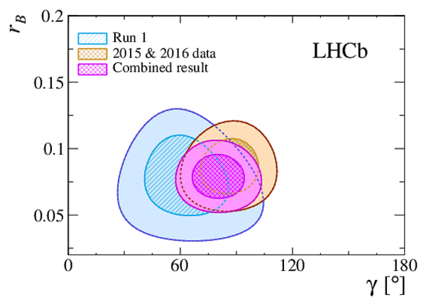
Two-dimensional 68.3 % and 95.5 % confidence regions for $( \gamma, r_B, \delta_B)$ for the $ x_{\pm}$ , $ y_{\pm}$ parameters obtained in the fit to 2015 and 2016 data, the fit to Run 1 data, and their combinations. |
Fig11left.pdf [15 KiB] HiDef png [377 KiB] Thumbnail [197 KiB] *.C file |
|
|
Fig11right.pdf [15 KiB] HiDef png [354 KiB] Thumbnail [194 KiB] *.C file |

|
|
|
Animated gif made out of all figures. |
PAPER-2018-017.gif Thumbnail |

|
![HiDef png [1 MiB]](Directory_LHCb-PAPER-2018-017/hidef_Fig1left.png)
![HiDef png [2 MiB]](Directory_LHCb-PAPER-2018-017/hidef_Fig1right.png)
![HiDef png [288 KiB]](Directory_LHCb-PAPER-2018-017/hidef_Fig2topleft.png)
![HiDef png [295 KiB]](Directory_LHCb-PAPER-2018-017/hidef_Fig2topright.png)
![HiDef png [180 KiB]](Directory_LHCb-PAPER-2018-017/hidef_Fig2bottomleft.png)
![HiDef png [182 KiB]](Directory_LHCb-PAPER-2018-017/hidef_Fig2bottomright.png)
![HiDef png [237 KiB]](Directory_LHCb-PAPER-2018-017/hidef_Fig3top.png)
![HiDef png [239 KiB]](Directory_LHCb-PAPER-2018-017/hidef_Fig3bottom.png)
![HiDef png [241 KiB]](Directory_LHCb-PAPER-2018-017/hidef_Fig4top.png)
![HiDef png [236 KiB]](Directory_LHCb-PAPER-2018-017/hidef_Fig4bottom.png)
![HiDef png [271 KiB]](Directory_LHCb-PAPER-2018-017/hidef_Fig5a.png)
![HiDef png [221 KiB]](Directory_LHCb-PAPER-2018-017/hidef_Fig5b.png)
![HiDef png [1 MiB]](Directory_LHCb-PAPER-2018-017/hidef_Fig6a.png)
![HiDef png [1 MiB]](Directory_LHCb-PAPER-2018-017/hidef_Fig6b.png)
![HiDef png [1 MiB]](Directory_LHCb-PAPER-2018-017/hidef_Fig6c.png)
![HiDef png [1 MiB]](Directory_LHCb-PAPER-2018-017/hidef_Fig6d.png)
![HiDef png [194 KiB]](Directory_LHCb-PAPER-2018-017/hidef_Fig7.png)
![HiDef png [113 KiB]](Directory_LHCb-PAPER-2018-017/hidef_Fig8left.png)
![HiDef png [117 KiB]](Directory_LHCb-PAPER-2018-017/hidef_Fig8right.png)
![HiDef png [1 MiB]](Directory_LHCb-PAPER-2018-017/hidef_Fig9left.png)
![HiDef png [2 MiB]](Directory_LHCb-PAPER-2018-017/hidef_Fig9right.png)
![HiDef png [356 KiB]](Directory_LHCb-PAPER-2018-017/hidef_Fig10.png)
![HiDef png [377 KiB]](Directory_LHCb-PAPER-2018-017/hidef_Fig11left.png)
![HiDef png [354 KiB]](Directory_LHCb-PAPER-2018-017/hidef_Fig11right.png)
Tables and captions
|
Statistical correlation matrix for the fit to data. |
Table_1.pdf [52 KiB] HiDef png [35 KiB] Thumbnail [16 KiB] tex code |

|
|
Fit results for the total $ B ^\pm \rightarrow D K ^\pm $ yields in the signal region, where the invariant mass of the $ B $ candidate is in the interval 5249--5319 $ {\mathrm{ Me V /}c^2}$ , integrated over the Dalitz plots. |
Table_2.pdf [65 KiB] HiDef png [34 KiB] Thumbnail [16 KiB] tex code |

|
|
Summary of uncertainties for the parameters $ x_{\pm}$ and $ y_{\pm}$ . The various sources of systematic uncertainties are described in the main text. All entries are given in multiples of $10^{-2}$. |
Table_3.pdf [71 KiB] HiDef png [84 KiB] Thumbnail [37 KiB] tex code |

|
|
Correlation matrix of the experimental and strong-phase related systematic uncertainties. |
Table_4.pdf [53 KiB] HiDef png [26 KiB] Thumbnail [13 KiB] tex code |

|
|
Correlation matrix between Run 1 results (I) and the results presented in this paper (II), when fitting data while varying the inputs from the CLEO collaboration in a correlated way. |
Table_5.pdf [58 KiB] HiDef png [65 KiB] Thumbnail [31 KiB] tex code |

|
|
Total correlation matrix for the systematic uncertainties of the Run 1 results (I) and the results presented in this paper (II), including experimental and strong phase related systematic uncertainties. |
Table_6.pdf [58 KiB] HiDef png [68 KiB] Thumbnail [32 KiB] tex code |

|
![HiDef png [35 KiB]](Directory_LHCb-PAPER-2018-017/hidef_Table_1.png)
![HiDef png [34 KiB]](Directory_LHCb-PAPER-2018-017/hidef_Table_2.png)
![HiDef png [84 KiB]](Directory_LHCb-PAPER-2018-017/hidef_Table_3.png)
![HiDef png [26 KiB]](Directory_LHCb-PAPER-2018-017/hidef_Table_4.png)
![HiDef png [65 KiB]](Directory_LHCb-PAPER-2018-017/hidef_Table_5.png)
![HiDef png [68 KiB]](Directory_LHCb-PAPER-2018-017/hidef_Table_6.png)
Supplementary Material [file]
| Supplementary material full pdf |
supple[..].pdf [188 KiB] |

|
|
This ZIP file contains supplemetary material for the publication LHCb-PAPER-2018-017. The files are: supplementary.pdf : An overview of the extra figures *.pdf, *.png, *.eps, *.C : The figures in variuous formats |
SupMat[..].pdf [15 KiB] HiDef png [276 KiB] Thumbnail [155 KiB] *C file |

|
|
SupMat[..].pdf [15 KiB] HiDef png [335 KiB] Thumbnail [185 KiB] *C file |

|
|
|
SupMatFig2.pdf [39 KiB] HiDef png [364 KiB] Thumbnail [235 KiB] *C file |
|
![HiDef png [276 KiB]](Directory_LHCb-PAPER-2018-017/supplementary/hidef_SupMatFig1left.png)
![HiDef png [335 KiB]](Directory_LHCb-PAPER-2018-017/supplementary/hidef_SupMatFig1right.png)
![HiDef png [364 KiB]](Directory_LHCb-PAPER-2018-017/supplementary/hidef_SupMatFig2.png)
Created on 02 May 2024.