Measurement of the relative $B^{-} \rightarrow D^{0} / D^{*0} / D^{**0} \mu^{-} \overline{\nu}_\mu$ branching fractions using $B^{-}$ mesons from $\overline{B}{}_{s2}^{*0}$ decays

Information

LHCb-PAPER-2018-024
CERN-EP-2018-190
arXiv:1807.10722 [PDF]

(Submitted on 27 Jul 2018)
Phys. Rev. D99 (2019) 092009
Inspire 1684260

Tools

Abstract

The decay of the narrow resonance $\overline{B}{}_{s2}^{*0} \rightarrow B^- K^+$ can be used to determine the $B^-$ momentum in partially reconstructed decays without any assumptions on the decay products of the $B^-$ meson. This technique is employed for the first time to distinguish contributions from $D^0$, $D^{*0}$, and higher-mass charmed states ($D^{**0}$) in semileptonic $B^-$ decays by using the missing-mass distribution. The measurement is performed using a data sample corresponding to an integrated luminosity of 3.0 fb${}^{-1}$ collected with the LHCb detector in $pp$ collisions at center-of-mass energies of 7 and 8 TeV. The resulting branching fractions relative to the inclusive $B^- \rightarrow D^0 X \mu^- \overline{\nu}_\mu$ are $f_{D^0} = \mathcal{B}( B^- \rightarrow D^0\mu^-\overline{\nu}_\mu )/\mathcal{B}( B^- \rightarrow D^0 X \mu^- \overline{\nu}_\mu ) = 0.25 \pm 0.06$, $f_{D^{**0}} = \mathcal{B}( B^- \rightarrow ( D^{**0} \rightarrow D^0 X)\mu^-\overline{\nu}_\mu )/\mathcal{B}( B^- \rightarrow D^0 X \mu^- \overline{\nu}_\mu ) = 0.21 \pm 0.07$, with $f_{D^{*0}} = 1 - f_{D^0} - f_{D^{**0}}$ making up the remainder.

Figures and captions

Decay topology for the $ { B ^- \rightarrow D ^0 X \mu ^- \overline{\nu } _\mu }$ signal decays. A $\overline{ B }{} {}_{s2}^{*0}$ meson decays at the primary vertex position, producing a $ B ^-$ meson and a $ K ^+$ meson. The angle in the laboratory frame between the $ K ^+$ and $ B ^-$ directions is defined as $\theta$. The $ B ^-$ meson then decays semileptonically to a $ D ^0$ meson and a muon, accompanied by an undetected neutrino and potentially other particles, referred to collectively as $X$.	Fig1.pdf [47 KiB] HiDef png [32 KiB] Thumbnail [17 KiB] *.C file
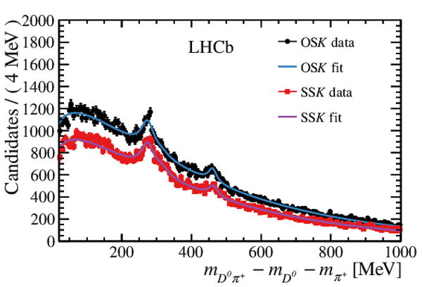
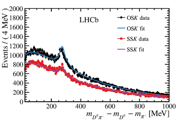
Distribution of the minimum mass difference for $ B ^- K ^+ $ (\text{OS} $ K $ ) candidates and $ B ^- K ^- $ (\text{SS} $ K $ ) candidates. For \text{OS} $ K $ combinations, peaks for the $\overline{ B }{} {}_{s2}^{*0}$ and $\overline{ B }{} {}_{s1}^0$ states are visible. The contribution of decays in which a kaon from a $b$-hadron decay is chosen as prompt produces the sharp increase near zero. The \text{SS} $ K $ sample is used for background estimation.	Fig2.pdf [24 KiB] HiDef png [199 KiB] Thumbnail [203 KiB] *.C file
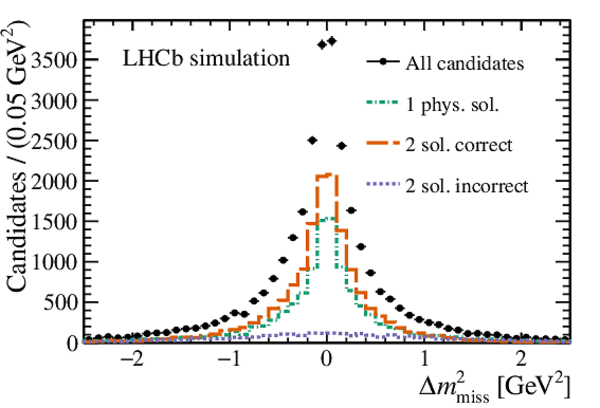
The difference $\Delta m_{\mathrm{miss}}^2 $ between the reconstructed missing mass squared and the corresponding true values for the (top left) $ { B ^- \rightarrow D ^0 \mu ^- \overline{\nu } _\mu }$ channel, (top right) the $ { B ^- \rightarrow D ^{0} \mu ^- \overline{\nu } _\mu }$ channel, and (bottom) the $ { B ^- \rightarrow D^{*0} \mu ^- \overline{\nu } _\mu }$ channel. The contributions from events in which there is only one physical solution, in which there are two and the chosen lower energy solution is correct, or in which the incorrect solution is chosen are shown.	Fig3a.pdf [17 KiB] HiDef png [244 KiB] Thumbnail [216 KiB] *.C file
	Fig3b.pdf [18 KiB] HiDef png [253 KiB] Thumbnail [227 KiB] *.C file
	Fig3c.pdf [17 KiB] HiDef png [237 KiB] Thumbnail [207 KiB] *.C file
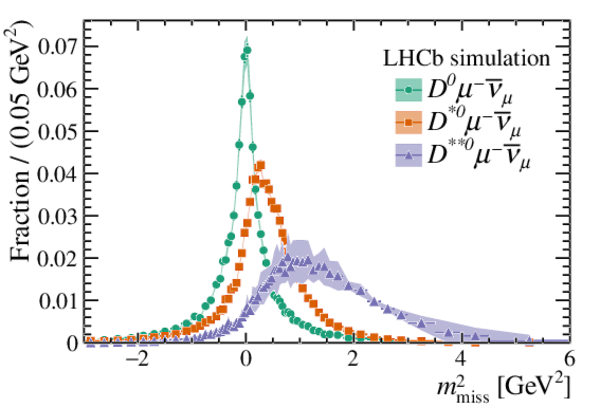
The missing mass shapes from simulation for the signal samples are shown. The bands around the points represent the systematic uncertainties on the form factors in the simulation and the branching fractions for different contributions to the $ D^{**0}$ channel.	Fig4.pdf [27 KiB] HiDef png [357 KiB] Thumbnail [242 KiB] *.C file
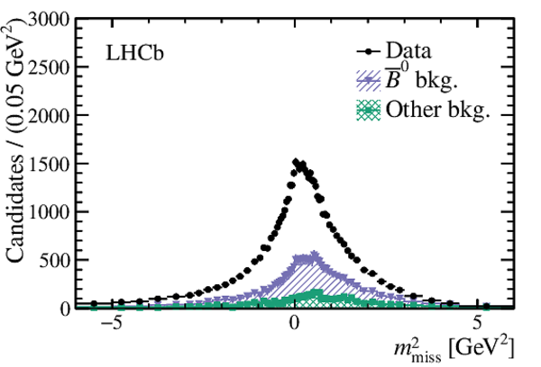
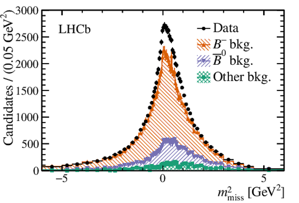
Missing-mass distribution for data and estimated background contributions in the (left) same-sign kaon sample and (right) opposite-sign sample. The other background decays include contributions from misreconstructed backgrounds, and semileptonic decays of $\overline{ B }{} {}^0_ s $ and $\Lambda ^0_ b $ mesons. The remainder of the \text{SS} $ K $ sample not from $\overline{ B }{} {}^0$ or other background decays is used to define the background contribution from $ B ^-$ semileptonic decays. This is then extrapolated to the \text{OS} $ K $ sample, where the remainder is composed of signal. The background distributions are stacked.	Fig5a.pdf [27 KiB] HiDef png [258 KiB] Thumbnail [193 KiB] *.C file
	Fig5b.pdf [32 KiB] HiDef png [479 KiB] Thumbnail [301 KiB] *.C file
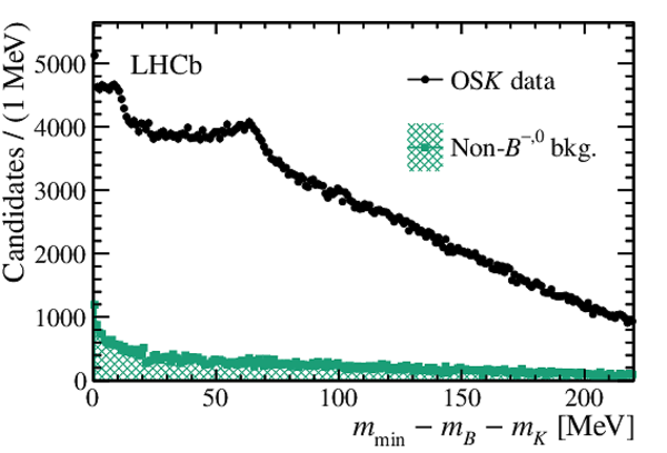
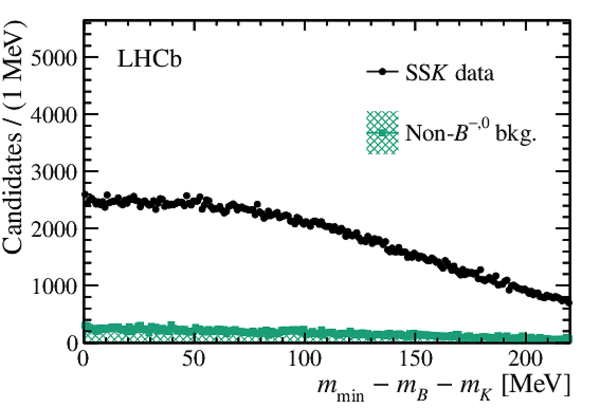
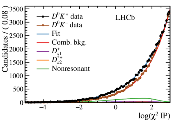
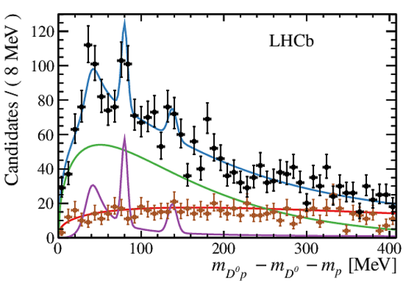
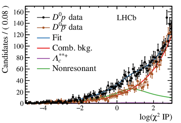
Distribution of the minimum mass difference for (left) $ B ^- K ^+ $ opposite-sign candidates and (right) $ B ^- K ^- $ same-sign candidates. All candidates are compared to the estimated background from other sources besides decays of a $ B ^-$ or $\overline{ B }{} {}^0$ meson to $ D ^0 X\mu ^- \overline{\nu } _\mu $. The remaining non-peaking part of the distributions is made up of $ B ^-$ and $\overline{ B }{} {}^0$ semileptonic decays that do not come from an excited $\overline{ B }{} {}^0_ s $ state.	Fig6a.pdf [30 KiB] HiDef png [269 KiB] Thumbnail [209 KiB] *.C file
	Fig6b.pdf [27 KiB] HiDef png [233 KiB] Thumbnail [192 KiB] *.C file
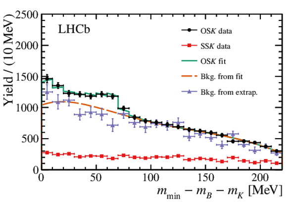
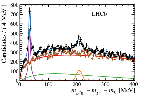
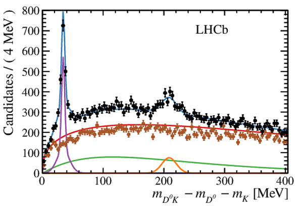
Fits to the opposite-sign and same-sign kaon $ m_{\mathrm{min}} - m_B - m_K$ distributions with non- $ B ^-$ and $\overline{ B }{} {}^0$ backgrounds subtracted, and the resulting estimations of the non- $\overline{ B }{} {}_{s2}^{*0}$ and $\overline{ B }{} {}_{s1}^0$ contributions. The fits are done separately in three bins of the prompt kaon $ p_{\mathrm{ T}}$ : (top left) $0.5 < p_{\mathrm{ T}} < 1.25\mathrm{ Ge V} $, (top right) $1.25 < p_{\mathrm{ T}} < 2\mathrm{ Ge V} $, and (bottom) $ p_{\mathrm{ T}} > 2\mathrm{ Ge V} $. The dashed line shows the background estimation using a fit to the full \text{OS} $ K $ distribution with signal templates from simulation and a fifth-order polynomial for the background. The points estimate the background using a linear extrapolation of the \text{OS} $ K $ to \text{SS} $ K $ ratio in the region $ m_{\mathrm{min}} - m_B - m_K > 100\mathrm{ Me V} $.	Fig7a.pdf [20 KiB] HiDef png [249 KiB] Thumbnail [193 KiB] *.C file
	Fig7b.pdf [20 KiB] HiDef png [243 KiB] Thumbnail [190 KiB] *.C file
	Fig7c.pdf [20 KiB] HiDef png [269 KiB] Thumbnail [202 KiB] *.C file
Template fit to the missing-mass distribution. The nuisance parameters used to quantify the template statistical uncertainties are set to their nominal values. The full distribution (left) is shown, comparing the background to the sum of the signal templates. The background-subtracted distribution (right) is compared to the breakdown of the signal components. The statistical uncertainty in the background templates is represented as the shaded band around the fit. In the pull distribution, the statistical uncertainty of the background templates is added to the statistical uncertainty of the data points.	Fig8a.pdf [38 KiB] HiDef png [446 KiB] Thumbnail [323 KiB] *.C file
	Fig8b.pdf [32 KiB] HiDef png [454 KiB] Thumbnail [329 KiB] *.C file
Contours for 68.3% and 95.5% confidence intervals for the fractions of $ { B ^- \rightarrow D ^0 X \mu ^- \overline{\nu } _\mu }$ into the exclusive $ { B ^- \rightarrow D ^0 \mu ^- \overline{\nu } _\mu }$ channel and the higher excited $ { B ^- \rightarrow \left( { D^{0} \rightarrow D ^0 X} \right)\mu ^- \overline{\nu } _\mu }$ channels. The alternate fit using different branching fractions for different $ D^{0}$ states is not included.	Fig9.pdf [14 KiB] HiDef png [168 KiB] Thumbnail [137 KiB] *.C file
Animated gif made out of all figures.	PAPER-2018-024.gif Thumbnail

Tables and captions

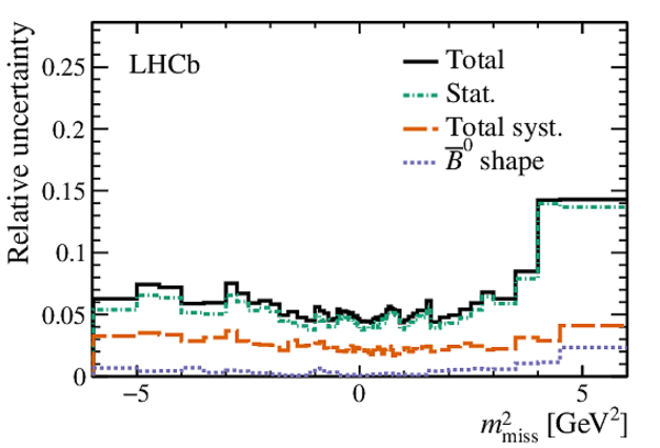
Estimates of the breakdown of the total uncertainty. All estimates are done by repeating the fit with systematic nuisance parameters fixed to their best fit values. The statistical uncertainty of the \text{OS} $ K $ sample is estimated from the uncertainty on the signal fractions with the template statistical nuisance parameters fixed to their best fit values. The template statistical uncertainty is added in by allowing only the statistical nuisance parameters to vary. The effect of each floating systematic uncertainty is estimated by refitting with its systematic nuisance parameter shifted by the uncertainty found by the best fit and taking the difference in the signal fractions as the uncertainty. The total uncertainty is taken from the best fit, with the fixed systematic uncertainties added in quadrature.

Table_1.pdf [70 KiB]
HiDef png [91 KiB]
Thumbnail [39 KiB]
tex code

Supplementary Material [file]

Supplementary material full pdf	Supple[..].pdf [575 KiB]
his ZIP file contains supplemetary material for the publication LHCb-PAPER-2018-024. The files are: Supplementary.pdf : An overview of the extra figures .pdf, .png, *.eps : The figures in various formats	Fig1-S.pdf [15 KiB] HiDef png [209 KiB] Thumbnail [181 KiB] *C file
	Fig2a-S.pdf [45 KiB] HiDef png [447 KiB] Thumbnail [267 KiB] *C file
	Fig2b-S.pdf [46 KiB] HiDef png [259 KiB] Thumbnail [195 KiB] *C file
	Fig2c-S.pdf [45 KiB] HiDef png [448 KiB] Thumbnail [273 KiB] *C file
	Fig2d-S.pdf [46 KiB] HiDef png [269 KiB] Thumbnail [200 KiB] *C file
	Fig3a-S.pdf [29 KiB] HiDef png [447 KiB] Thumbnail [271 KiB] *C file
	Fig3b-S.pdf [43 KiB] HiDef png [368 KiB] Thumbnail [259 KiB] *C file
	Fig3c-S.pdf [28 KiB] HiDef png [397 KiB] Thumbnail [248 KiB] *C file
	Fig3d-S.pdf [43 KiB] HiDef png [350 KiB] Thumbnail [245 KiB] *C file
	Fig4a-S.pdf [34 KiB] HiDef png [244 KiB] Thumbnail [171 KiB] *C file
	Fig4b-S.pdf [82 KiB] HiDef png [340 KiB] Thumbnail [245 KiB] *C file
	Fig4c-S.pdf [57 KiB] HiDef png [330 KiB] Thumbnail [242 KiB] *C file