Search for beautiful tetraquarks in the $\Upsilon(1S)\mu^+\mu^-$ invariant-mass spectrum
[to restricted-access page]Information
LHCb-PAPER-2018-027
CERN-EP-2018-163
arXiv:1806.09707 [PDF]
(Submitted on 25 Jun 2018)
JHEP 10 (2018) 086
Inspire 1679857
Tools
Abstract
The $\Upsilon(1S)\mu^+\mu^-$ invariant-mass distribution is investigated for a possible exotic meson state composed of two $b$ quarks and two $\overline{b}$ quarks, $X_{b\overline{b}b\overline{b}}$. The analysis is based on a data sample of $pp$ collisions recorded with the LHCb detector at centre-of-mass energies $\sqrt{s} =$ 7, 8 and 13 TeV, corresponding to an integrated luminosity of 6.3 fb$^{-1}$. No significant excess is found, and upper limits are set on the product of the production cross-section and the branching fraction as functions of the mass of the $X_{b\overline{b}b\overline{b}}$ state. The limits are set in the fiducial volume where all muons have pseudorapidity in the range $[2.0,5.0]$, and the $X_{b\overline{b}b\overline{b}}$ state has rapidity in the range $[2.0,4.5]$ and transverse momentum less than 15 GeV/$c$.
Figures and captions
|
Linear fit to the ratio of the $X$ and $\Y1S$ widths as a function of the $X$ mass as determined from fits to simulated data samples. The error bars represent the statistical uncertainty arising from the finite size of the simulated samples. |
fig1a.pdf [14 KiB] HiDef png [130 KiB] Thumbnail [124 KiB] *.C file |

|
|
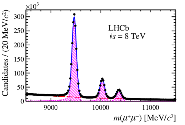
Distributions of $m(\mu ^+\mu ^- )$ for the normalisation datasets at $ p p $ centre-of-mass energies of (a) 7 $\mathrm{ Te V}$ , (b) 8 $\mathrm{ Te V}$ , (c) 13 $\mathrm{ Te V}$ and (d) all combined. The total fit function (solid blue line), the combinatorial background (dashed red line) and the $\Y1S$, $\Y2S$ and $\Y3S$ components (hatched magenta area) are shown overlaid. |
fig2a.pdf [49 KiB] HiDef png [229 KiB] Thumbnail [167 KiB] *.C file |

|
|
fig2b.pdf [49 KiB] HiDef png [233 KiB] Thumbnail [172 KiB] *.C file |
|
|
|
fig2c.pdf [49 KiB] HiDef png [245 KiB] Thumbnail [187 KiB] *.C file |

|
|
|
fig2d.pdf [49 KiB] HiDef png [239 KiB] Thumbnail [179 KiB] *.C file |

|
|
|
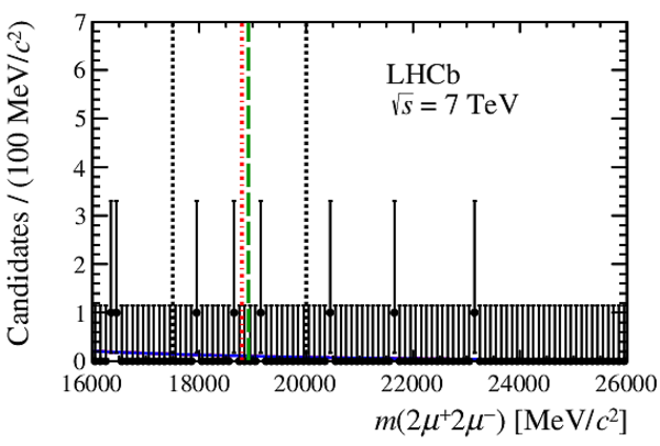
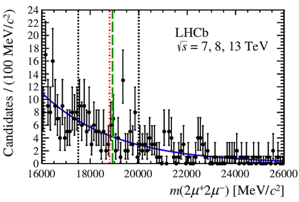
Distributions of $m(2\mu^+2\mu^-)$ for the signal datasets at $ p p $ centre-of-mass energies of (a) 7 $\mathrm{ Te V}$ , (b) 8 $\mathrm{ Te V}$ , (c) 13 $\mathrm{ Te V}$ and (d) all combined, using a bin size comparable to the expected $X$ mass resolution. In each case the region around the corresponding $\Y1S$ peak has been selected. The background-only fit function (solid blue line) is shown overlaid. The dotted black lines indicate the range in which limits are set on the product of the $X$ production cross-section and branching fractions. The dash-dotted red and long-dashed green lines show the positions of the $\eta_b\eta_b$ and $\Y1S\Y1S$ thresholds, respectively. |
fig3a.pdf [26 KiB] HiDef png [202 KiB] Thumbnail [189 KiB] *.C file |
|
|
fig3b.pdf [27 KiB] HiDef png [223 KiB] Thumbnail [208 KiB] *.C file |

|
|
|
fig3c.pdf [31 KiB] HiDef png [255 KiB] Thumbnail [246 KiB] *.C file |

|
|
|
fig3d.pdf [31 KiB] HiDef png [259 KiB] Thumbnail [250 KiB] *.C file |
|
|
|
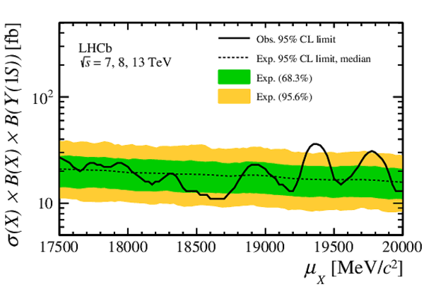
The 95 % CL upper limits on $S\equiv \sigma( p p \rightarrow X)\times\mathcal{B}(X\rightarrow \Y1S\mu ^+\mu ^- ) \times \mathcal{B}(\Y1S\rightarrow \mu^+\mu^-)$ as functions of the $X$ mass hypothesis at $ p p $ centre-of-mass energies of (a) 7 $\mathrm{ Te V}$ , (b) 8 $\mathrm{ Te V}$ and (c) 13 $\mathrm{ Te V}$ and (d) all combined. |
fig4a.pdf [17 KiB] HiDef png [189 KiB] Thumbnail [154 KiB] *.C file |

|
|
fig4b.pdf [17 KiB] HiDef png [215 KiB] Thumbnail [170 KiB] *.C file |

|
|
|
fig4c.pdf [17 KiB] HiDef png [236 KiB] Thumbnail [187 KiB] *.C file |

|
|
|
fig4d.pdf [17 KiB] HiDef png [237 KiB] Thumbnail [189 KiB] *.C file |
|
|
|
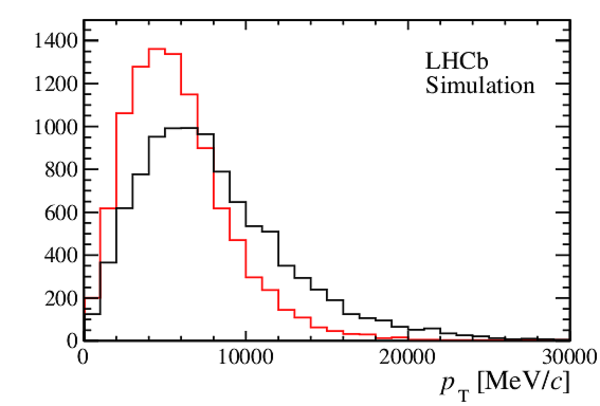
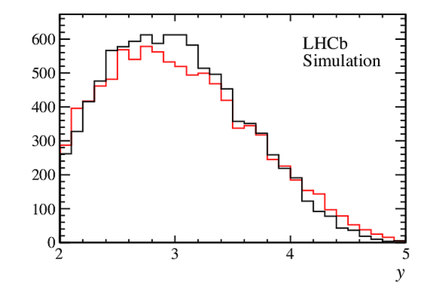
The kinematic distribution of (black) simulated $X$ particles in (a) $ p_{\mathrm{ T}} $ and (b) rapidity, and (c) the 2D distribution. For comparison, the kinematic distribution of (red) simulated $\Y4S$ particles is also shown. |
fig5a.pdf [13 KiB] HiDef png [106 KiB] Thumbnail [109 KiB] *.C file |
|
|
fig5b.pdf [12 KiB] HiDef png [52 KiB] Thumbnail [53 KiB] *.C file |
|
|
|
fig5c.pdf [13 KiB] HiDef png [84 KiB] Thumbnail [89 KiB] *.C file |
|
|
|
fig5d.pdf [20 KiB] HiDef png [212 KiB] Thumbnail [195 KiB] *.C file |

|
|
|
Animated gif made out of all figures. |
PAPER-2018-027.gif Thumbnail |

|
![HiDef png [130 KiB]](Directory_LHCb-PAPER-2018-027/hidef_fig1a.png)
![HiDef png [229 KiB]](Directory_LHCb-PAPER-2018-027/hidef_fig2a.png)
![HiDef png [233 KiB]](Directory_LHCb-PAPER-2018-027/hidef_fig2b.png)
![HiDef png [245 KiB]](Directory_LHCb-PAPER-2018-027/hidef_fig2c.png)
![HiDef png [239 KiB]](Directory_LHCb-PAPER-2018-027/hidef_fig2d.png)
![HiDef png [202 KiB]](Directory_LHCb-PAPER-2018-027/hidef_fig3a.png)
![HiDef png [223 KiB]](Directory_LHCb-PAPER-2018-027/hidef_fig3b.png)
![HiDef png [255 KiB]](Directory_LHCb-PAPER-2018-027/hidef_fig3c.png)
![HiDef png [259 KiB]](Directory_LHCb-PAPER-2018-027/hidef_fig3d.png)
![HiDef png [189 KiB]](Directory_LHCb-PAPER-2018-027/hidef_fig4a.png)
![HiDef png [215 KiB]](Directory_LHCb-PAPER-2018-027/hidef_fig4b.png)
![HiDef png [236 KiB]](Directory_LHCb-PAPER-2018-027/hidef_fig4c.png)
![HiDef png [237 KiB]](Directory_LHCb-PAPER-2018-027/hidef_fig4d.png)
![HiDef png [106 KiB]](Directory_LHCb-PAPER-2018-027/hidef_fig5a.png)
![HiDef png [52 KiB]](Directory_LHCb-PAPER-2018-027/hidef_fig5b.png)
![HiDef png [84 KiB]](Directory_LHCb-PAPER-2018-027/hidef_fig5c.png)
![HiDef png [212 KiB]](Directory_LHCb-PAPER-2018-027/hidef_fig5d.png)
Tables and captions
|
Upper limits on $\sigma( p p \rightarrow X) \times \mathcal{B}(X\rightarrow \Y1S\mu ^+\mu ^- ) \times \mathcal{B}(\Y1S\rightarrow \mu ^+\mu ^- )$ for different $X$ mass hypotheses in the range $[17.5,18.4] {\mathrm{ Ge V /}c^2} $. |
Table_1.pdf [46 KiB] HiDef png [487 KiB] Thumbnail [233 KiB] tex code |

|
|
Upper limits on $\sigma( p p \rightarrow X) \times \mathcal{B}(X\rightarrow \Y1S\mu ^+\mu ^- ) \times \mathcal{B}(\Y1S\rightarrow \mu ^+\mu ^- )$ for different $X$ mass hypotheses in the range $[18.4,19.3] {\mathrm{ Ge V /}c^2} $. |
Table_2.pdf [46 KiB] HiDef png [470 KiB] Thumbnail [226 KiB] tex code |

|
|
Upper limits on $\sigma( p p \rightarrow X) \times \mathcal{B}(X\rightarrow \Y1S\mu ^+\mu ^- ) \times \mathcal{B}(\Y1S\rightarrow \mu ^+\mu ^- )$ for different $X$ mass hypotheses in the range $[19.3,20.0] {\mathrm{ Ge V /}c^2} $. |
Table_3.pdf [46 KiB] HiDef png [402 KiB] Thumbnail [190 KiB] tex code |

|
![HiDef png [487 KiB]](Directory_LHCb-PAPER-2018-027/hidef_Table_1.png)
![HiDef png [470 KiB]](Directory_LHCb-PAPER-2018-027/hidef_Table_2.png)
![HiDef png [402 KiB]](Directory_LHCb-PAPER-2018-027/hidef_Table_3.png)
Created on 26 April 2024.