Measurement of the branching fractions of the decays $D^+\rightarrow K^-K^+K^+$, $D^+\rightarrow \pi^-\pi^+K^+$ and $D^+_s\rightarrow\pi^-K^+K^+$

Information

LHCb-PAPER-2018-033
CERN-EP-2018-244
arXiv:1810.03138 [PDF]

(Submitted on 07 Oct 2018)
JHEP 03 (2019) 176
Inspire 1697372

Tools

Abstract

The branching fractions of the doubly Cabibbo-suppressed decays $D^+\rightarrow K^-K^+K^+$, $D^+\rightarrow \pi^-\pi^+K^+$ and $D^+_s\rightarrow\pi^-K^+K^+$ are measured using the decays $D^+\rightarrow K^-\pi^+\pi^+$ and $D^+_s\rightarrow K^-K^+\pi^+$ as normalisation channels. The measurements are performed using proton-proton collision data collected with the LHCb detector at a centre-of-mass energy of 8 TeV, corresponding to an integrated luminosity of 2.0 fb$^{-1}$. The results are \begin{align} \frac {\mathcal{B}(D^+\rightarrow K^-K^+K^+)} {\mathcal{B}(D^+\rightarrow K^-\pi^+\pi^+)}& = (6.541 \pm 0.025 \pm 0.042) \times 10^{-4},\nonumber \frac {\mathcal{B}(D^+\rightarrow \pi^-\pi^+K^+)} {\mathcal{B}(D^+\rightarrow K^-\pi^+\pi^+)}& = (5.231 \pm 0.009 \pm 0.023) \times 10^{-3}, \nonumber \frac {\mathcal{B}(D^+_s\rightarrow\pi^-K^+K^+)} {\mathcal{B}(D^+_s\rightarrow K^-K^+\pi^+)}& = (2.372 \pm 0.024 \pm 0.025) \times 10^{-3},\nonumber \end{align} where the uncertainties are statistical and systematic, respectively. These are the most precise measurements up to date.

Figures and captions

Feynman diagrams for the DCS decays (a) $ D ^+ \rightarrow K ^- K ^+ K ^+ $ , (b) $ D ^+ \rightarrow \pi ^- \pi ^+ K ^+ $ and (c) $ D ^+_ s \rightarrow \pi ^- K ^+ K ^+ $ .	Fig1a.png [10 KiB] HiDef png [24 KiB] Thumbnail [13 KiB] *.C file
	Fig1b.png [9 KiB] HiDef png [23 KiB] Thumbnail [14 KiB] *.C file
	Fig1c.png [8 KiB] HiDef png [23 KiB] Thumbnail [14 KiB] *.C file
Efficiency maps for (top left) $ D ^+ \rightarrow K ^- K ^+ K ^+ $ , (top right) $ D ^+ \rightarrow \pi ^- \pi ^+ K ^+ $ , (middle left) $ D ^+_ s \rightarrow \pi ^- K ^+ K ^+ $ , (middle right) $ D ^+ \rightarrow K ^- K ^+ \pi ^+ $ , (bottom left) $ D ^+ \rightarrow K ^- \pi ^+ \pi ^+ $ and (bottom right) $ D ^+_ s \rightarrow K ^- K ^+ \pi ^+ $ decays with PID efficiency, tracking, multiplicity and hardware trigger efficiency corrections, for MagDown polarity.	Fig2a.pdf [14 KiB] HiDef png [139 KiB] Thumbnail [120 KiB] *.C file
	Fig2b.pdf [15 KiB] HiDef png [167 KiB] Thumbnail [141 KiB] *.C file
	Fig2c.pdf [16 KiB] HiDef png [195 KiB] Thumbnail [179 KiB] *.C file
	Fig2d.pdf [17 KiB] HiDef png [213 KiB] Thumbnail [203 KiB] *.C file
	Fig2e.pdf [17 KiB] HiDef png [208 KiB] Thumbnail [201 KiB] *.C file
	Fig2f.pdf [15 KiB] HiDef png [142 KiB] Thumbnail [119 KiB] *.C file
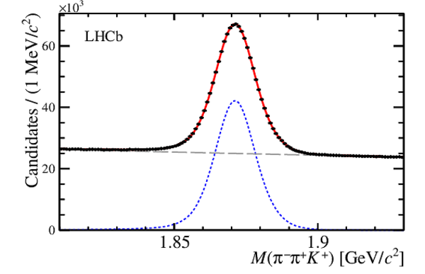
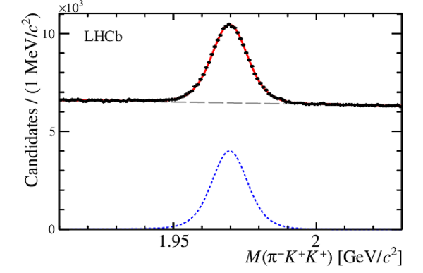
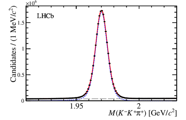
Invariant-mass distributions of (top left) $ D ^+ \rightarrow K ^- K ^+ K ^+ $ , (top right) $ D ^+ \rightarrow \pi ^- \pi ^+ K ^+ $ , (bottom left) $ D ^+_ s \rightarrow \pi ^- K ^+ K ^+ $ and (bottom right) $ D ^+ \rightarrow K ^- K ^+ \pi ^+ $ with the corresponding fit result superimposed (red solid line). The blue dotted line corresponds to the signal PDF and the dashed grey line shows the background PDF.	Fig3a.pdf [38 KiB] HiDef png [144 KiB] Thumbnail [117 KiB] *.C file
	Fig3b.pdf [37 KiB] HiDef png [142 KiB] Thumbnail [115 KiB] *.C file
	Fig3c.pdf [38 KiB] HiDef png [124 KiB] Thumbnail [101 KiB] *.C file
	Fig3d.pdf [38 KiB] HiDef png [147 KiB] Thumbnail [117 KiB] *.C file
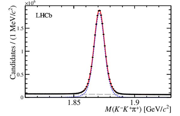
Invariant-mass distributions of candidates of the normalisation modes (left) $ D ^+ \rightarrow K ^- \pi ^+ \pi ^+ $ and (right) $ D ^+_ s \rightarrow K ^- K ^+ \pi ^+ $ with the corresponding fit result superimposed (red solid line). The blue dotted line corresponds to the signal PDF and the dashed grey line shows the background PDF.	Fig4a.pdf [37 KiB] HiDef png [129 KiB] Thumbnail [100 KiB] *.C file
	Fig4b.pdf [38 KiB] HiDef png [145 KiB] Thumbnail [113 KiB] *.C file
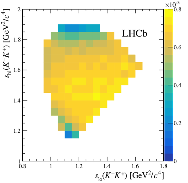
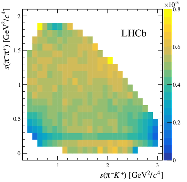
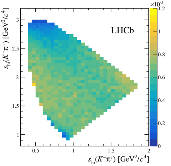
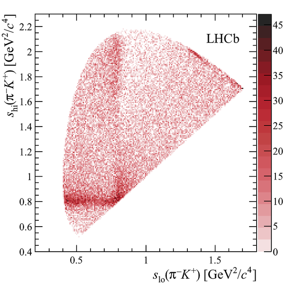
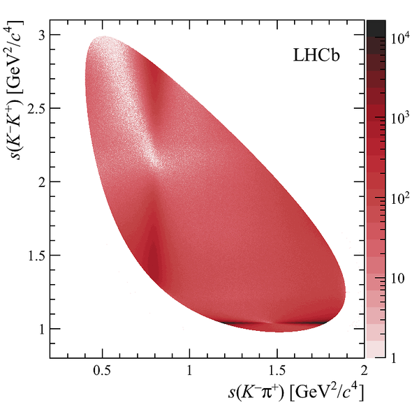
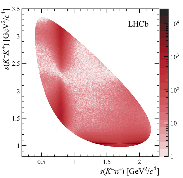
Dalitz plots of the (top left) $ D ^+ \rightarrow K ^- K ^+ K ^+ $ , (top right) $ D ^+ \rightarrow \pi ^- \pi ^+ K ^+ $ , where the $ K ^0_{\mathrm{ \scriptscriptstyle S}}$ veto can be seen, (middle left) $ D ^+_ s \rightarrow \pi ^- K ^+ K ^+ $ , (middle right) $ D ^+ \rightarrow K ^- K ^+ \pi ^+ $ , (bottom left) $ D ^+ \rightarrow K ^- \pi ^+ \pi ^+ $ and (bottom right) $ D ^+_ s \rightarrow K ^- K ^+ \pi ^+ $ decays, with signal weights from sPlot . A logarithmic scale is used for the $ D ^+ \rightarrow K ^- K ^+ \pi ^+ $ and $ D ^+_ s \rightarrow K ^- K ^+ \pi ^+ $ channels.	Fig5a.png [54 KiB] HiDef png [428 KiB] Thumbnail [219 KiB] *.C file
	Fig5b.png [165 KiB] HiDef png [788 KiB] Thumbnail [309 KiB] *.C file
	Fig5c.png [60 KiB] HiDef png [549 KiB] Thumbnail [233 KiB] *.C file
	Fig5d.png [117 KiB] HiDef png [480 KiB] Thumbnail [200 KiB] *.C file
	Fig5e.png [64 KiB] HiDef png [271 KiB] Thumbnail [128 KiB] *.C file
	Fig5f.png [145 KiB] HiDef png [622 KiB] Thumbnail [240 KiB] *.C file
Animated gif made out of all figures.	PAPER-2018-033.gif Thumbnail

Tables and captions

World averages for the branching-fractions ratios under consideration [3].	Table_1.pdf [66 KiB] HiDef png [52 KiB] Thumbnail [26 KiB] tex code
Ratios of average efficiencies for the full selection. The quoted uncertainty is due to the limited size of the simulated sample only (see Section 7).	Table_2.pdf [90 KiB] HiDef png [59 KiB] Thumbnail [29 KiB] tex code
Observed yields for signal and normalisation modes with statistical uncertainties. The entry for the decay $ D ^+ \rightarrow K ^- \pi ^+ \pi ^+ $ $^{(\dagger)}$ corresponds to the yields obtained from the fit to $ D ^+ \rightarrow K ^- \pi ^+ \pi ^+ $ sample with cuts optimised for the $ D ^+ \rightarrow K ^- K ^+ K ^+ $ and $ D ^+ \rightarrow K ^- K ^+ \pi ^+ $ selections. The entry for the decay $ D ^+ \rightarrow K ^- \pi ^+ \pi ^+ $ $^{(\dagger\dagger)}$ is for fits to $ D ^+ \rightarrow K ^- \pi ^+ \pi ^+ $ samples with cuts optimised for the $ D ^+ \rightarrow \pi ^- \pi ^+ K ^+ $ selection.	Table_3.pdf [78 KiB] HiDef png [80 KiB] Thumbnail [39 KiB] tex code
Produced yields for each decay mode with statistical uncertainties, shown separately for MagDown and Mag Up samples. The numbers given for the decay $ D ^+ \rightarrow K ^- \pi ^+ \pi ^+ $ $^{(\dagger)}$ correspond to the sample with cuts optimised for the $ D ^+ \rightarrow K ^- K ^+ K ^+ $ and $ D ^+ \rightarrow K ^- K ^+ \pi ^+ $ and those for the decay $ D ^+ \rightarrow K ^- \pi ^+ \pi ^+ $ { $^{(\dagger\dagger)}$} to the sample with cuts optimised for the $ D ^+ \rightarrow \pi ^- \pi ^+ K ^+ $ selection.	Table_4.pdf [98 KiB] HiDef png [103 KiB] Thumbnail [52 KiB] tex code
Relative systematic uncertainties for the MagDown and Mag Up results (in %). The statistical uncertainties are also given for comparison.	Table_5.pdf [94 KiB] HiDef png [125 KiB] Thumbnail [53 KiB] tex code
Ratios of branching fractions, shown separately for MagDown and Mag Up samples. The first uncertainty is statistical and the second is systematic.	Table_6.pdf [103 KiB] HiDef png [116 KiB] Thumbnail [61 KiB] tex code