Evidence for an $\eta_c(1S) \pi^-$ resonance in $B^0 \to \eta_c(1S) K^+\pi^-$ decays

Information

LHCb-PAPER-2018-034
CERN-EP-2018-245
arXiv:1809.07416 [PDF]

(Submitted on 19 Sep 2018)
Eur. Phys. J. C78 (2018) 1019
Inspire 1694990

Tools

Abstract

A Dalitz plot analysis of $B^0 \to \eta_c(1S) K^+\pi^-$ decays is performed using data samples of $pp$ collisions collected with the LHCb detector at centre-of-mass energies of $\sqrt{s}=7, 8$ and $13$ TeV, corresponding to a total integrated luminosity of $4.7 \text{fb}^{-1}$. A satisfactory description of the data is obtained when including a contribution representing an exotic $\eta_c(1S) \pi^-$ resonant state. The significance of this exotic resonance is more than three standard deviations, while its mass and width are $4096 \pm 20 ^{+18}_{-22}$ MeV and $152 \pm 58 ^{+60}_{-35}$ MeV, respectively. The spin-parity assignments $J^P=0^+$ and $J^{P}=1^-$ are both consistent with the data. In addition, the first measurement of the $B^0 \to \eta_c(1S) K^+\pi^-$ branching fraction is performed and gives $\displaystyle \mathcal{B}(B^0 \to \eta_c(1S) K^+\pi^-) = (5.73 \pm 0.24 \pm 0.13 \pm 0.66) \times 10^{-4}$, where the first uncertainty is statistical, the second systematic, and the third is due to limited knowledge of external branching fractions.

Figures and captions

Feynman diagrams for \subref{B2etacKstar} $B^0 \rightarrow \eta_cK^{*0}$ and \subref{B2ZK} $B^0 \rightarrow Z_c^-K^+$ decay sequences.	Fig1a.pdf [24 KiB] HiDef png [33 KiB] Thumbnail [16 KiB] *.C file
	Fig1b.pdf [150 KiB] HiDef png [35 KiB] Thumbnail [19 KiB] *.C file
Distribution of the $ p $ $\overline p $ $ K ^+$ $\pi ^-$ invariant mass. The solid blue curve is the projection of the total fit result. The components are shown in the legend.	Fig2.pdf [38 KiB] HiDef png [260 KiB] Thumbnail [223 KiB] *.C file
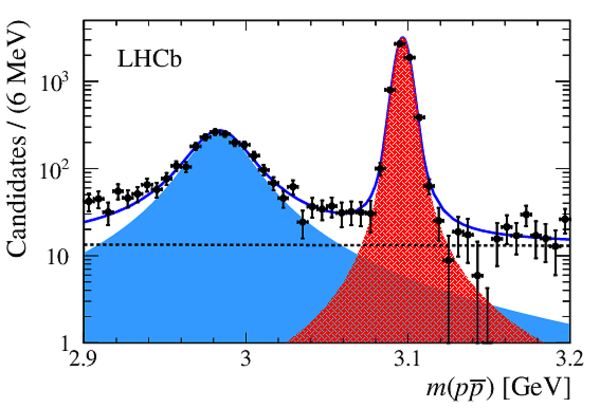
Distribution of the $ p $ $\overline p $ invariant mass in (left) linear and (right) logarithmic vertical-axis scale for weighted $ B ^0 \rightarrow p \overline p K ^+ \pi ^- $ candidates obtained by using the sPlot technique. The solid blue curve is the projection of the total fit result. The full azure, tight-cross-hatched red and dashed-black line areas show the $\eta _ c $ , $ { J \mskip -3mu/\mskip -2mu\psi \mskip 2mu}$ and NR $ p $ $\overline p $ contributions, respectively.	Fig3a.pdf [22 KiB] HiDef png [285 KiB] Thumbnail [206 KiB] *.C file
	Fig3b.pdf [21 KiB] HiDef png [580 KiB] Thumbnail [290 KiB] *.C file
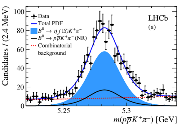
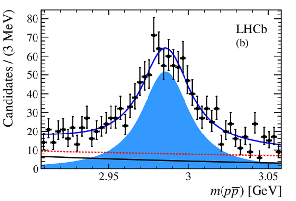
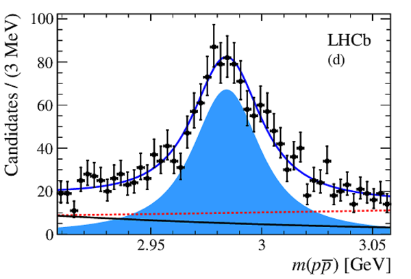
Results of the 2D mass fit to the joint [$ m( p \overline p K ^+ \pi ^- )$, $ m( p \overline p )$] distribution for the (a) Run 1 $ m( p \overline p K ^+ \pi ^- )$ projection, (b) Run 1 $ m( p \overline p )$ projection, (c) Run 2 $ m( p \overline p K ^+ \pi ^- )$ projection, and (d) Run 2 $ m( p \overline p )$ projection. The legend is shown in the top left plot.	Fig4a.pdf [21 KiB] HiDef png [277 KiB] Thumbnail [234 KiB] *.C file
	Fig4c.pdf [20 KiB] HiDef png [241 KiB] Thumbnail [197 KiB] *.C file
	Fig4b.pdf [21 KiB] HiDef png [249 KiB] Thumbnail [212 KiB] *.C file
	Fig4d.pdf [20 KiB] HiDef png [244 KiB] Thumbnail [199 KiB] *.C file
SDP distributions used in the DP fit to the Run 2 subsample for (a) combinatorial background and (b) NR $ B ^0 \rightarrow p \overline p K ^+ \pi ^- $ background.	Fig5a.pdf [20 KiB] HiDef png [161 KiB] Thumbnail [139 KiB] *.C file
	Fig5b.pdf [19 KiB] HiDef png [156 KiB] Thumbnail [139 KiB] *.C file
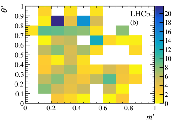
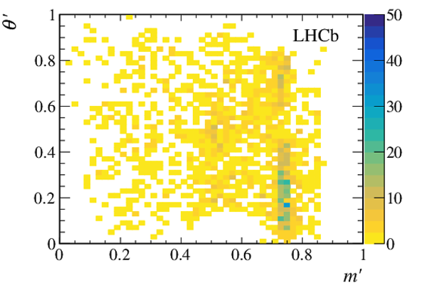
Background-subtracted (top) DP and (bottom) SDP distributions corresponding to the total data sample used in the analysis. The structure corresponding to the $K^*(892)^0$ resonance is evident. The veto of $ B ^0 \rightarrow \eta _ c K ^+ \pi ^- $ decays in the $\overline{ D }{} {}^0$ region is visible in the DP.	Fig6a.pdf [17 KiB] HiDef png [243 KiB] Thumbnail [270 KiB] *.C file
	Fig6b.pdf [17 KiB] HiDef png [232 KiB] Thumbnail [261 KiB] *.C file
$ B ^0 \rightarrow \eta _ c K ^+ \pi ^- $ signal efficiency across the SDP for the (a) Run 1 and (b) Run 2 samples.	Fig7a.pdf [20 KiB] HiDef png [220 KiB] Thumbnail [168 KiB] *.C file
	Fig7b.pdf [20 KiB] HiDef png [220 KiB] Thumbnail [169 KiB] *.C file
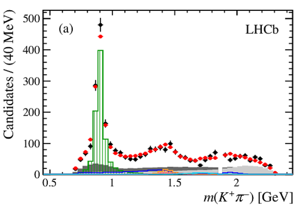
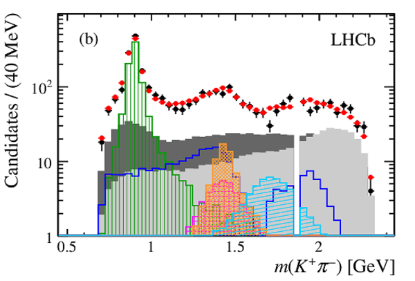
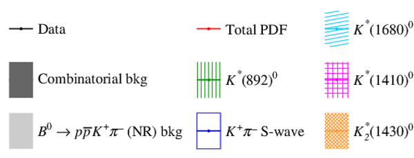
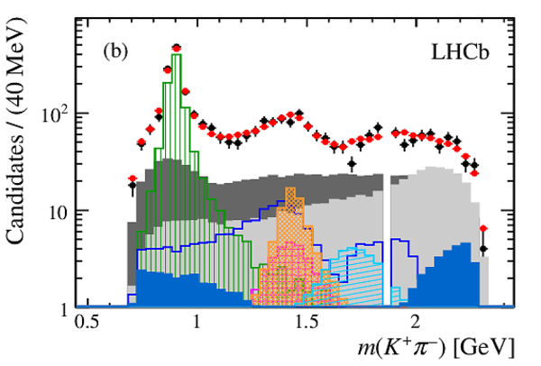
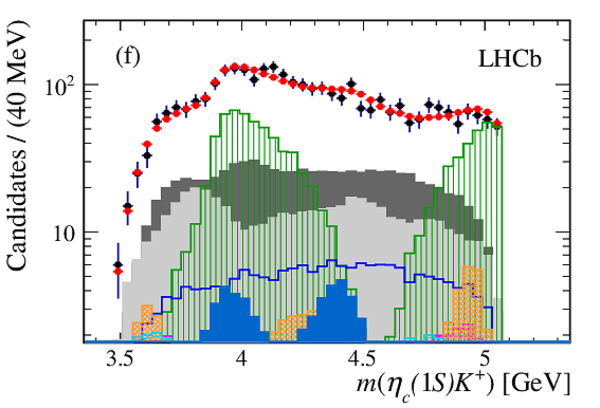
Projections of the data and amplitude fit using the baseline model onto (a) $ m( K ^+ \pi ^- )$, (c) $ m(\eta _ c \pi ^- )$ and (e) $ m(\eta _ c K ^+ )$, with the same projections shown in (b), (d) and (f) with a logarithmic vertical-axis scale. The veto of $ B ^0 \rightarrow p \overline p \overline{ D }{} {}^0 $ decays is visible in plot (b). The $ K ^+ \pi ^- $ S-wave component comprises the LASS and $K^*_0(1950)^0$ meson contributions. The components are described in the legend at the bottom.	Fig8a.pdf [23 KiB] HiDef png [170 KiB] Thumbnail [148 KiB] *.C file
	Fig8b.pdf [24 KiB] HiDef png [428 KiB] Thumbnail [237 KiB] *.C file
	Fig8c.pdf [24 KiB] HiDef png [273 KiB] Thumbnail [220 KiB] *.C file
	Fig8d.pdf [26 KiB] HiDef png [920 KiB] Thumbnail [385 KiB] *.C file
	Fig8e.pdf [24 KiB] HiDef png [280 KiB] Thumbnail [219 KiB] *.C file
	Fig8f.pdf [24 KiB] HiDef png [411 KiB] Thumbnail [244 KiB] *.C file
	Fig8g.pdf [13 KiB] HiDef png [141 KiB] Thumbnail [99 KiB] *.C file
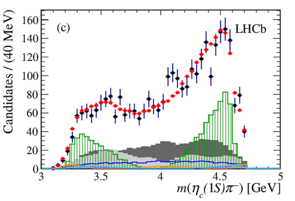
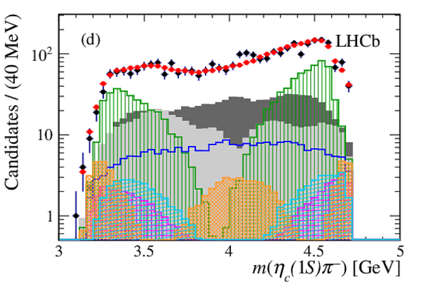
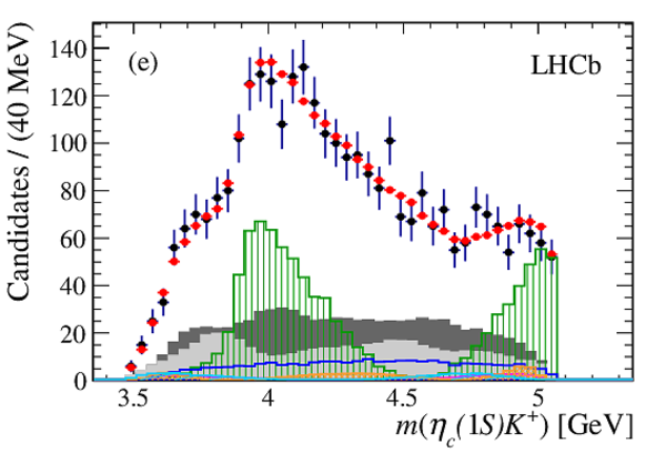
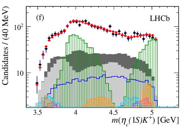
Projections of the data and amplitude fit using the nominal model onto (a) $ m( K ^+ \pi ^- )$, (c) $ m(\eta _ c \pi ^- )$ and (e) $ m(\eta _ c K ^+ )$, with the same projections shown in (b), (d) and (f) with a logarithmic vertical-axis scale. The veto of $ B ^0 \rightarrow p \overline p \overline{ D }{} {}^0 $ decays is visible in plot (b). The $ K ^+ \pi ^- $ S-wave component comprises the LASS and $K^*_0(1950)^0$ meson contributions. The components are described in the legend at the bottom.	Fig9a.pdf [23 KiB] HiDef png [167 KiB] Thumbnail [145 KiB] *.C file
	Fig9b.pdf [24 KiB] HiDef png [402 KiB] Thumbnail [230 KiB] *.C file
	Fig9c.pdf [24 KiB] HiDef png [253 KiB] Thumbnail [212 KiB] *.C file
	Fig9d.pdf [26 KiB] HiDef png [627 KiB] Thumbnail [304 KiB] *.C file
	Fig9e.pdf [24 KiB] HiDef png [256 KiB] Thumbnail [211 KiB] *.C file
	Fig9f.pdf [24 KiB] HiDef png [328 KiB] Thumbnail [220 KiB] *.C file
	Fig9g.pdf [13 KiB] HiDef png [135 KiB] Thumbnail [99 KiB] *.C file
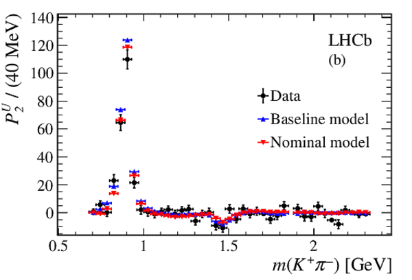
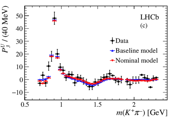
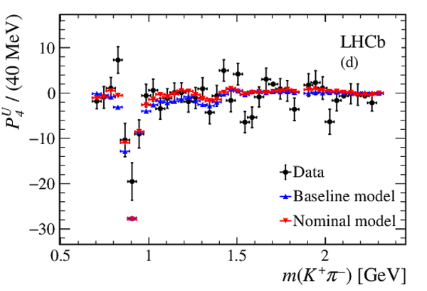
Comparison of the first four $ K ^+ \pi ^- $ Legendre moments determined from background-subtracted data (black points) and from the results of the amplitude fit using the baseline model (red triangles) and nominal model (blue triangles) as a function of $ m( K ^+ \pi ^- )$.	Fig10a.pdf [22 KiB] HiDef png [179 KiB] Thumbnail [150 KiB] *.C file
	Fig10b.pdf [23 KiB] HiDef png [190 KiB] Thumbnail [164 KiB] *.C file
	Fig10c.pdf [22 KiB] HiDef png [195 KiB] Thumbnail [173 KiB] *.C file
	Fig10d.pdf [22 KiB] HiDef png [194 KiB] Thumbnail [169 KiB] *.C file
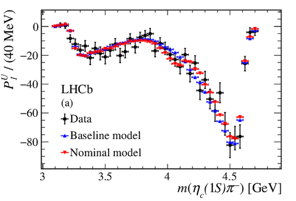
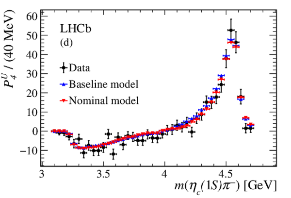
Comparison of the first four $\eta _ c \pi ^- $ Legendre moments determined from background-subtracted data (black points) and from the results of the amplitude fit using the baseline model (red triangles) and nominal model (blue triangles) as a function of $ m(\eta _ c \pi ^- )$.	Fig11a.pdf [23 KiB] HiDef png [210 KiB] Thumbnail [180 KiB] *.C file
	Fig11b.pdf [23 KiB] HiDef png [217 KiB] Thumbnail [197 KiB] *.C file
	Fig11c.pdf [23 KiB] HiDef png [210 KiB] Thumbnail [190 KiB] *.C file
	Fig11d.pdf [23 KiB] HiDef png [206 KiB] Thumbnail [184 KiB] *.C file
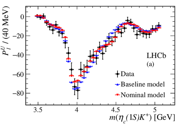
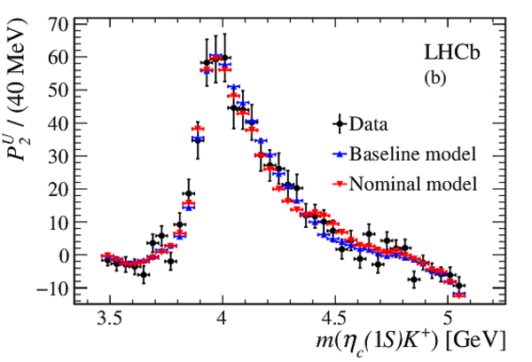
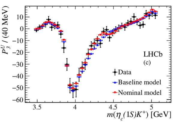
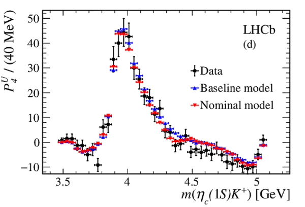
Comparison of the first four $\eta _ c K ^+ $ Legendre moments determined from background-subtracted data (black points) and from the results of the amplitude fit using the baseline model (red triangles) and nominal model (blue triangles) as a function of $ m(\eta _ c K ^+ )$.	Fig12a.pdf [22 KiB] HiDef png [210 KiB] Thumbnail [179 KiB] *.C file
	Fig12b.pdf [23 KiB] HiDef png [219 KiB] Thumbnail [197 KiB] *.C file
	Fig12c.pdf [23 KiB] HiDef png [216 KiB] Thumbnail [193 KiB] *.C file
	Fig12d.pdf [22 KiB] HiDef png [213 KiB] Thumbnail [189 KiB] *.C file
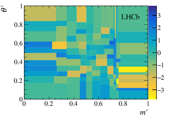
2D pull distribution for to the baseline model.	Fig13.pdf [22 KiB] HiDef png [169 KiB] Thumbnail [135 KiB] *.C file
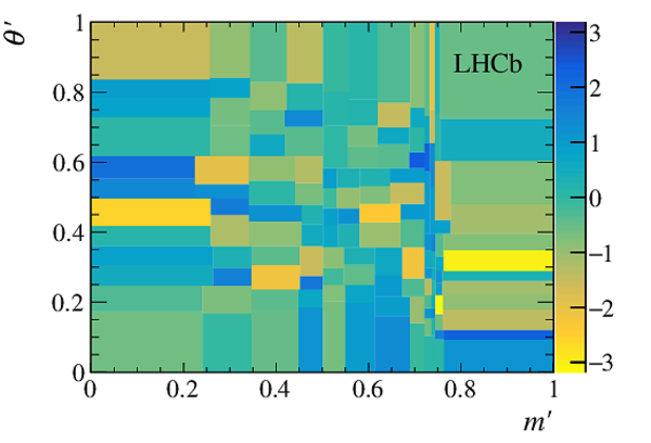
2D pull distribution for to the nominal model.	Fig14.pdf [22 KiB] HiDef png [170 KiB] Thumbnail [136 KiB] *.C file
Animated gif made out of all figures.	PAPER-2018-034.gif Thumbnail

Tables and captions

Relative systematic uncertainties on the ratio $R$ of Eq. \eqref{ratio}. The total systematic uncertainty is obtained from the quadratic sum of the individual sources.	Table_1.pdf [40 KiB] HiDef png [47 KiB] Thumbnail [21 KiB] tex code
Yields of the components in the 2D mass fit to the joint [$ m( p \overline p K ^+ \pi ^- )$, $ m( p \overline p )$] distribution for the Run 1 and 2 subsamples.	Table_2.pdf [69 KiB] HiDef png [49 KiB] Thumbnail [23 KiB] tex code
Resonances included in the baseline model, where parameters and uncertainties are taken from Ref. \cite{PDG2016}. The LASS lineshape also parametrise the $ K ^+ \pi ^- $ S-wave in $ B ^0 \rightarrow \eta _ c K ^+ \pi ^- $ NR decays.	Table_3.pdf [69 KiB] HiDef png [83 KiB] Thumbnail [41 KiB] tex code
Complex coefficients and fit fractions determined from the DP fit using the nominal model. Uncertainties are statistical only.	Table_4.pdf [71 KiB] HiDef png [92 KiB] Thumbnail [44 KiB] tex code
Significance of the $Z_c(4100)^-$ contribution for the systematic effects producing the largest variations in the parameters of the $Z_c(4100)^-$ candidate. The values obtained in the nominal amplitude fit are shown in the first row.	Table_5.pdf [71 KiB] HiDef png [63 KiB] Thumbnail [28 KiB] tex code
Rejection level of the $J^P=0^+$ hypothesis with respect to the $J^P=1^-$ hypothesis for the systematic variations producing the largest variations in the parameters of the $Z_c(4100)^-$ candidate. The values obtained in the nominal amplitude fit are shown in the first row.	Table_6.pdf [70 KiB] HiDef png [60 KiB] Thumbnail [27 KiB] tex code
Fit fractions and their uncertainties. The quoted uncertainties are statistical and systematic, respectively.	Table_7.pdf [71 KiB] HiDef png [119 KiB] Thumbnail [58 KiB] tex code
Branching fraction results. The four quoted uncertainties are statistical, $ B ^0 \rightarrow \eta _ c K ^+ \pi ^- $ branching fraction systematic (not including the contribution from the uncertainty associated to the efficiency ratio, to avoid double counting the systematic uncertainty associated to the evaluation of the efficiencies), fit fraction systematic and external branching fractions uncertainties, respectively.	Table_8.pdf [71 KiB] HiDef png [78 KiB] Thumbnail [37 KiB] tex code
Symmetric matrix of the fit fractions (%) from the amplitude fit using the nominal model. The quoted uncertainties are statistical and systematic, respectively. The diagonal elements correspond to the values reported in Table ???.	Table_9.pdf [66 KiB] HiDef png [42 KiB] Thumbnail [20 KiB] tex code