Searches for 25 rare and forbidden decays of $D^{+}$ and $ {D}_s^{+} $ mesons
[to restricted-access page]Information
LHCb-PAPER-2020-007
CERN-EP-2020-140
arXiv:2011.00217 [PDF]
(Submitted on 31 Oct 2020)
JHEP 06 (2021) 044
Inspire 1827570
Tools
Abstract
A search is performed for rare and forbidden charm decays of the form $D_{(s)}^+ \to h^\pm \ell^+ \ell^{(\prime)\mp}$, where $h^\pm$ is a pion or kaon and $\ell^{(')\pm}$ is an electron or muon. The measurements are performed using proton-proton collision data, corresponding to an integrated luminosity of $1.6\text{fb}^{-1}$, collected by the LHCb experiment in 2016. No evidence is observed for the 25 decay modes that are investigated and $90\%$ confidence level limits on the branching fractions are set between $1.4\times10^{-8}$ and $6.4\times10^{-6}$. In most cases, these results represent an improvement on existing limits by one to two orders of magnitude.
Figures and captions
|
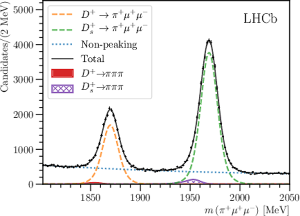
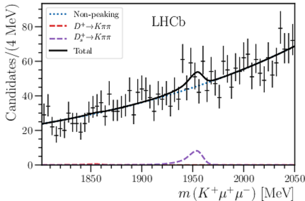
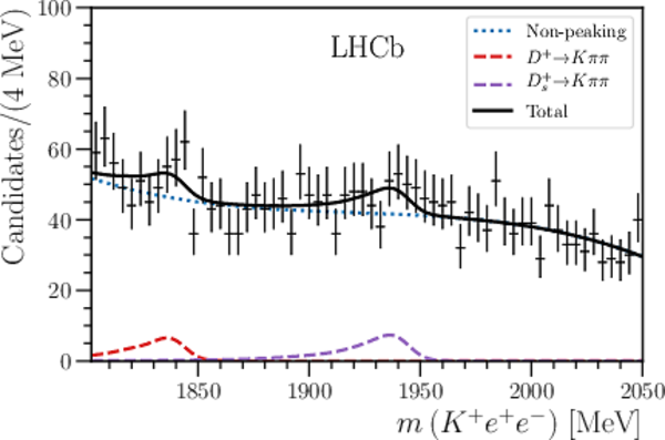
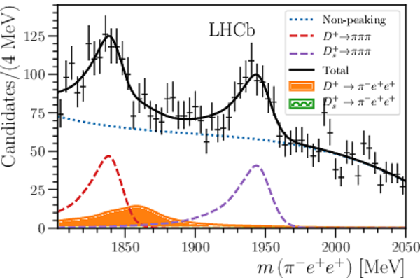
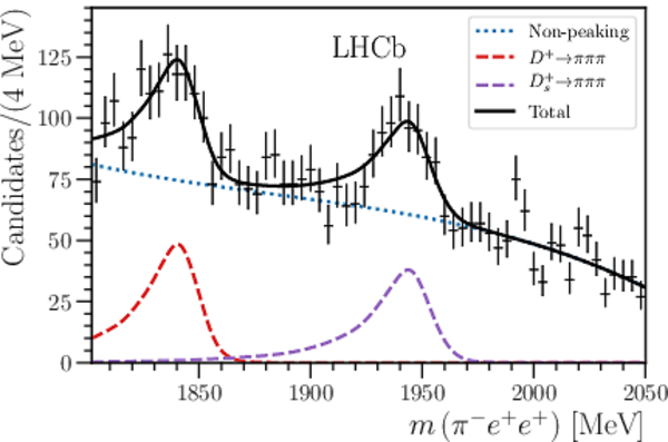
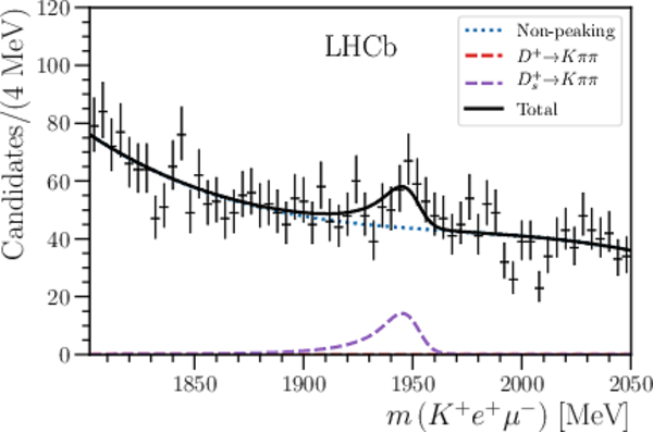
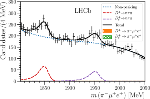
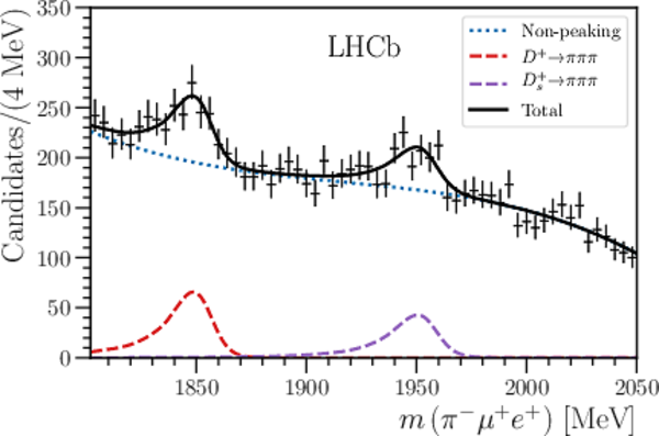
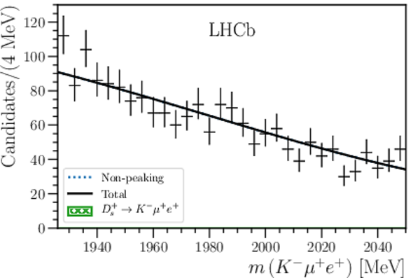
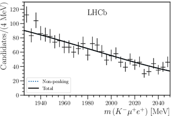
Distributions of the three-body invariant mass for the $ D ^+_{(s)} \rightarrow \left(\phi \rightarrow \ell^-\ell^+ \right)$ $\pi ^+$ candidates used for normalisation and calibration. The final states are specified in the mass label. The $ D ^+$ ( $ D ^+_ s $ ) signal component is shown as a dashed orange (green) line, peaking backgrounds are denoted by the solid (hashed) regions and the non-peaking background is denoted by the blue dotted line. |
Fig1a.pdf [557 KiB] HiDef png [297 KiB] Thumbnail [207 KiB] |
|
|
Fig1b.pdf [555 KiB] HiDef png [312 KiB] Thumbnail [242 KiB] |

|
|
|
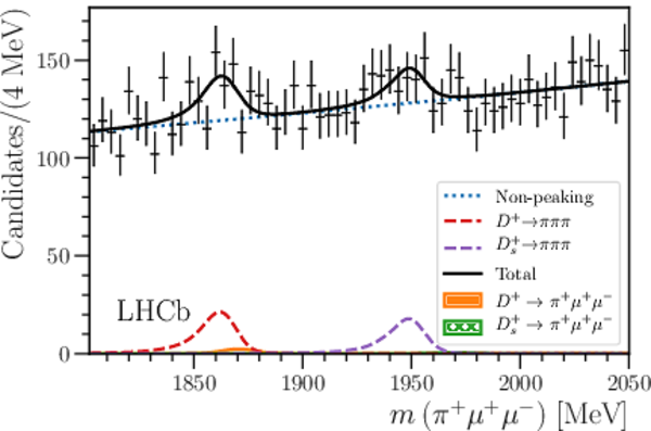
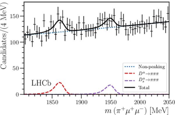
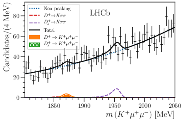
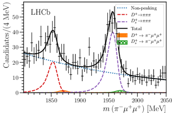
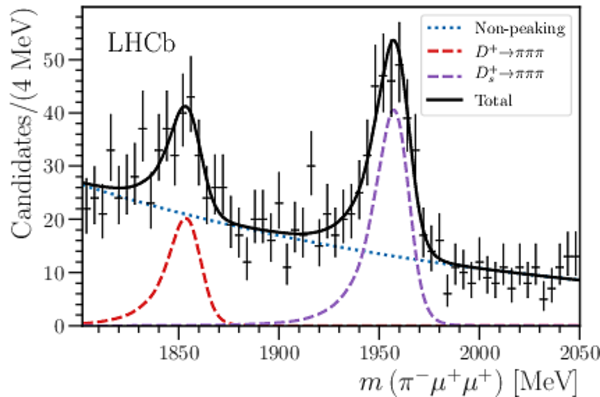
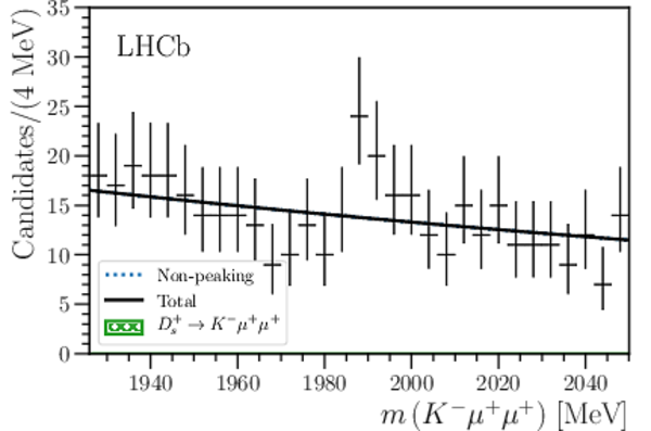
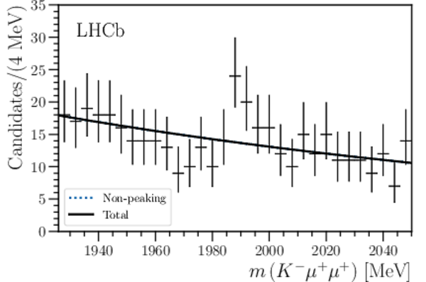
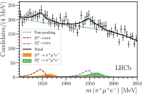
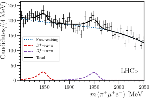
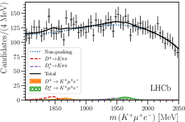
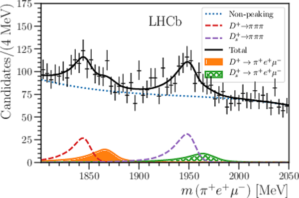
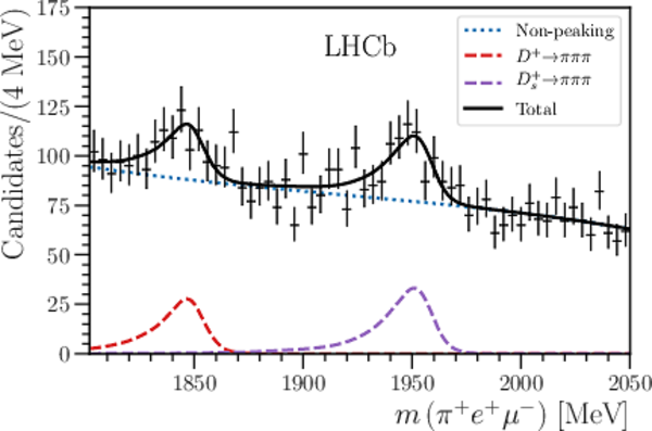
Distributions of the three-body invariant mass in the signal regions for decays with two muons. The final states are specified in the mass label. The left (right) fit with the signal-plus-background (background-only) hypothesis is overlaid with the peaking backgrounds denoted by dashed lines and the non-peaking background is denoted by the blue dotted line. |
Fig2a.pdf [582 KiB] HiDef png [217 KiB] Thumbnail [196 KiB] |
|
|
Fig2b.pdf [330 KiB] HiDef png [197 KiB] Thumbnail [179 KiB] |
|
|
|
Fig2c.pdf [567 KiB] HiDef png [212 KiB] Thumbnail [194 KiB] |
|
|
|
Fig2d.pdf [329 KiB] HiDef png [185 KiB] Thumbnail [172 KiB] |
|
|
|
Fig2e.pdf [594 KiB] HiDef png [289 KiB] Thumbnail [243 KiB] |
|
|
|
Fig2f.pdf [331 KiB] HiDef png [259 KiB] Thumbnail [224 KiB] |
|
|
|
Fig2g.pdf [267 KiB] HiDef png [156 KiB] Thumbnail [141 KiB] |
|
|
|
Fig2h.pdf [128 KiB] HiDef png [145 KiB] Thumbnail [131 KiB] |
|
|
|
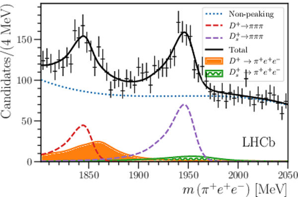
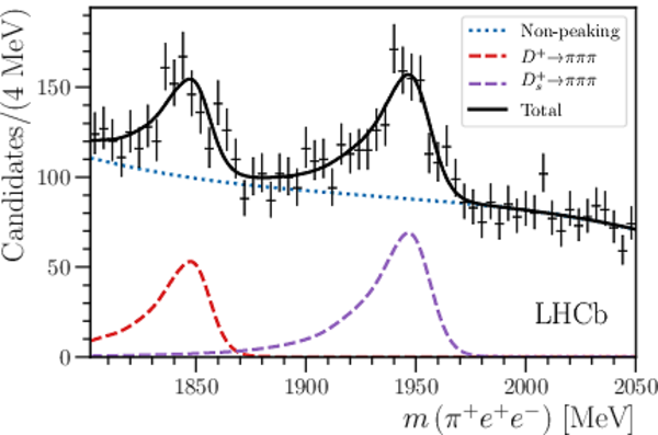
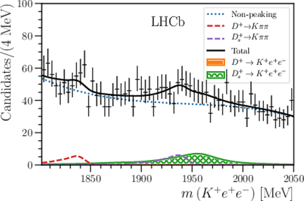
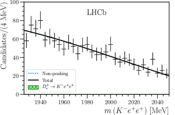
Distributions of the three-body invariant mass in the signal regions for decays with two electrons. The final states are specified in the mass label. The left (right) fit with the signal-plus-background (background-only) hypothesis is overlaid with the peaking backgrounds denoted by dashed lines and the non-peaking background is denoted by the blue dotted line. |
Fig3a.pdf [619 KiB] HiDef png [296 KiB] Thumbnail [235 KiB] |
|
|
Fig3b.pdf [331 KiB] HiDef png [229 KiB] Thumbnail [200 KiB] |
|
|
|
Fig3c.pdf [581 KiB] HiDef png [274 KiB] Thumbnail [219 KiB] |
|
|
|
Fig3d.pdf [330 KiB] HiDef png [201 KiB] Thumbnail [182 KiB] |
|
|
|
Fig3e.pdf [582 KiB] HiDef png [273 KiB] Thumbnail [233 KiB] |
|
|
|
Fig3f.pdf [331 KiB] HiDef png [231 KiB] Thumbnail [204 KiB] |
|
|
|
Fig3g.pdf [269 KiB] HiDef png [153 KiB] Thumbnail [138 KiB] |
|
|
|
Fig3h.pdf [128 KiB] HiDef png [142 KiB] Thumbnail [130 KiB] |
|
|
|
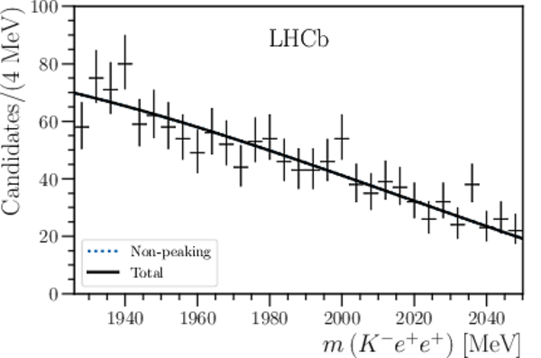
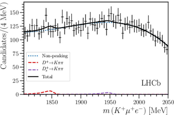
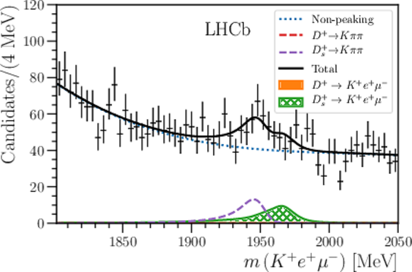
Distributions of the three-body invariant mass in the signal regions for decays with an oppositely charged electron and muon. The final states are specified in the mass label. The left (right) fit with the signal-plus-background (background-only) hypothesis is overlaid with the peaking backgrounds denoted by dashed lines and the non-peaking background is denoted by the blue dotted line. |
Fig4a.pdf [613 KiB] HiDef png [262 KiB] Thumbnail [214 KiB] |
|
|
Fig4b.pdf [330 KiB] HiDef png [206 KiB] Thumbnail [183 KiB] |
|
|
|
Fig4c.pdf [609 KiB] HiDef png [236 KiB] Thumbnail [202 KiB] |
|
|
|
Fig4d.pdf [330 KiB] HiDef png [194 KiB] Thumbnail [178 KiB] |
|
|
|
Fig4e.pdf [615 KiB] HiDef png [280 KiB] Thumbnail [226 KiB] |
|
|
|
Fig4f.pdf [330 KiB] HiDef png [217 KiB] Thumbnail [194 KiB] |
|
|
|
Fig4g.pdf [579 KiB] HiDef png [248 KiB] Thumbnail [207 KiB] |
|
|
|
Fig4h.pdf [329 KiB] HiDef png [192 KiB] Thumbnail [179 KiB] |
|
|
|
Distributions of the three-body invariant mass in the signal regions for decays with an electron and a muon with matching charge. The final states are specified in the mass label. The left (right) fit with the signal-plus-background (background-only) hypothesis is overlaid with the peaking backgrounds denoted by dashed lines and the non-peaking background is denoted by the blue dotted line. |
Fig5a.pdf [558 KiB] HiDef png [234 KiB] Thumbnail [205 KiB] |
|
|
Fig5b.pdf [331 KiB] HiDef png [216 KiB] Thumbnail [190 KiB] |
|
|
|
Fig5c.pdf [268 KiB] HiDef png [155 KiB] Thumbnail [141 KiB] |
|
|
|
Fig5d.pdf [128 KiB] HiDef png [143 KiB] Thumbnail [132 KiB] |
|
|
|
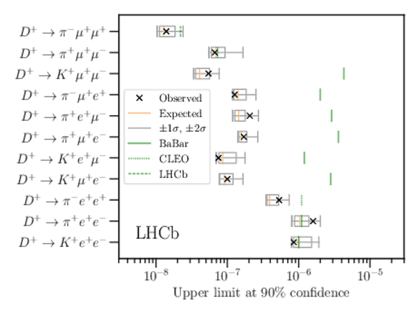
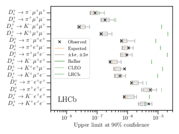
Upper limits at \SI{90}{\percent} confidence level on the $ D ^+_{(s)}$ signal channels. The median (orange), $\pm1\sigma$ and $\pm2\sigma$ expected limits are shown as box plots and the observed limit is given by a black cross. The green line shows the previous world's best limit for each channel where the solid, dotted and dashed lines correspond to BaBar, CLEO and LHCb \cite{Lees:2011hb,Rubin:2010cq,LHCB-PAPER-2012-051}. |
Fig6a.pdf [162 KiB] HiDef png [166 KiB] Thumbnail [143 KiB] |
|
|
Fig6b.pdf [196 KiB] HiDef png [194 KiB] Thumbnail [166 KiB] |
|
|
|
Animated gif made out of all figures. |
PAPER-2020-007.gif Thumbnail |

|
![HiDef png [297 KiB]](Directory_LHCb-PAPER-2020-007/hidef_Fig1a.png)
![HiDef png [312 KiB]](Directory_LHCb-PAPER-2020-007/hidef_Fig1b.png)
![HiDef png [217 KiB]](Directory_LHCb-PAPER-2020-007/hidef_Fig2a.png)
![HiDef png [197 KiB]](Directory_LHCb-PAPER-2020-007/hidef_Fig2b.png)
![HiDef png [212 KiB]](Directory_LHCb-PAPER-2020-007/hidef_Fig2c.png)
![HiDef png [185 KiB]](Directory_LHCb-PAPER-2020-007/hidef_Fig2d.png)
![HiDef png [289 KiB]](Directory_LHCb-PAPER-2020-007/hidef_Fig2e.png)
![HiDef png [259 KiB]](Directory_LHCb-PAPER-2020-007/hidef_Fig2f.png)
![HiDef png [156 KiB]](Directory_LHCb-PAPER-2020-007/hidef_Fig2g.png)
![HiDef png [145 KiB]](Directory_LHCb-PAPER-2020-007/hidef_Fig2h.png)
![HiDef png [296 KiB]](Directory_LHCb-PAPER-2020-007/hidef_Fig3a.png)
![HiDef png [229 KiB]](Directory_LHCb-PAPER-2020-007/hidef_Fig3b.png)
![HiDef png [274 KiB]](Directory_LHCb-PAPER-2020-007/hidef_Fig3c.png)
![HiDef png [201 KiB]](Directory_LHCb-PAPER-2020-007/hidef_Fig3d.png)
![HiDef png [273 KiB]](Directory_LHCb-PAPER-2020-007/hidef_Fig3e.png)
![HiDef png [231 KiB]](Directory_LHCb-PAPER-2020-007/hidef_Fig3f.png)
![HiDef png [153 KiB]](Directory_LHCb-PAPER-2020-007/hidef_Fig3g.png)
![HiDef png [142 KiB]](Directory_LHCb-PAPER-2020-007/hidef_Fig3h.png)
![HiDef png [262 KiB]](Directory_LHCb-PAPER-2020-007/hidef_Fig4a.png)
![HiDef png [206 KiB]](Directory_LHCb-PAPER-2020-007/hidef_Fig4b.png)
![HiDef png [236 KiB]](Directory_LHCb-PAPER-2020-007/hidef_Fig4c.png)
![HiDef png [194 KiB]](Directory_LHCb-PAPER-2020-007/hidef_Fig4d.png)
![HiDef png [280 KiB]](Directory_LHCb-PAPER-2020-007/hidef_Fig4e.png)
![HiDef png [217 KiB]](Directory_LHCb-PAPER-2020-007/hidef_Fig4f.png)
![HiDef png [248 KiB]](Directory_LHCb-PAPER-2020-007/hidef_Fig4g.png)
![HiDef png [192 KiB]](Directory_LHCb-PAPER-2020-007/hidef_Fig4h.png)
![HiDef png [234 KiB]](Directory_LHCb-PAPER-2020-007/hidef_Fig5a.png)
![HiDef png [216 KiB]](Directory_LHCb-PAPER-2020-007/hidef_Fig5b.png)
![HiDef png [155 KiB]](Directory_LHCb-PAPER-2020-007/hidef_Fig5c.png)
![HiDef png [143 KiB]](Directory_LHCb-PAPER-2020-007/hidef_Fig5d.png)
![HiDef png [166 KiB]](Directory_LHCb-PAPER-2020-007/hidef_Fig6a.png)
![HiDef png [194 KiB]](Directory_LHCb-PAPER-2020-007/hidef_Fig6b.png)
Tables and captions
|
Reference branching fractions ($\mathcal{B}$) used for the resonant channels alongside signal yields. |
Table_1.pdf [76 KiB] HiDef png [54 KiB] Thumbnail [28 KiB] tex code |

|
|
Summary of systematic uncertainties for each signal decay. The " $\phi \rightarrow \mu ^- \mu ^+ $ yield" column represents the combination of the statistical uncertainty from the $ D ^+_{(s)} \rightarrow \left(\phi \rightarrow \mu ^- \mu ^+ \right)$ $\pi ^+$ dataset with the systematic uncertainty from the modelling of the $ D ^+_{(s)} \rightarrow \pi ^+ \pi ^+ \pi ^- $ backgrounds. A further \SI{7.6}{\percent} uncertainty from the branching fraction of $ D ^+_{(s)} \rightarrow \left(\phi \rightarrow \mu ^- \mu ^+ \right)$ $\pi ^+$ and a \SI{1.0}{\percent} uncertainty from the finite size of the simulated $ D ^+_{(s)} \rightarrow \left(\phi \rightarrow \mu ^- \mu ^+ \right)$ $\pi ^+$ sample apply to all channels. The electron efficiency correction, described at the end of Section ???, is denoted by $\epsilon_{\text{electron}}$. All values are given in percent as a fractional uncertainty on the signal yield. |
Table_2.pdf [71 KiB] HiDef png [82 KiB] Thumbnail [33 KiB] tex code |

|
|
The single event sensitivities (SES), and upper limits on the branching fractions obtained using the CL$_s$ method, for each signal decay channel. |
Table_3.pdf [70 KiB] HiDef png [121 KiB] Thumbnail [54 KiB] tex code |

|
![HiDef png [54 KiB]](Directory_LHCb-PAPER-2020-007/hidef_Table_1.png)
![HiDef png [82 KiB]](Directory_LHCb-PAPER-2020-007/hidef_Table_2.png)
![HiDef png [121 KiB]](Directory_LHCb-PAPER-2020-007/hidef_Table_3.png)
Created on 27 April 2024.